Search in book...
Toggle Font Controls
Create new playlist

Name your new playlist

Playlist description (optional)
Sign In

Email address

Password

Forgot Password?

or

Continue with Facebook

Continue with Google
Sign Up

Full Name

Email address

Confirm Email Address

Password

or

Continue with Facebook

Continue with Google

Chapter Two

Environmental Impact Assessment of Different Renewable Energy Resources

A Recent Development

M.M. Rahman, S. Salehin, S.S.U. Ahmed, and A.K.M. Sadrul Islam Islamic University of Technology, Gazipur, Bangladesh

Abstract

For a sustainable development of human civilization, a secure and sufficient energy supply is very crucial. Global energy demand is expected to grow substantially, which will lead to increased production of energy from various sources. Conventional energy sources (e.g., oil, coal, and natural gas) drive economic progress, but utilization of these sources produces significant amounts of greenhouse gases that are responsible for global warming and ozone layer depletion. Policy regulations, such as California's low carbon fuel standard and European Union's fuel quality directive, encourage energy generation from cleaner sources. Renewable energy sources (e.g., solar, wind, biomass, hydro, and geothermal) are cleaner and easily accessible compared to conventional sources of energy. The potential of renewable energy sources is enormous. Renewable energy sector is growing faster and providing sustainable energy services. In this chapter, environmental impact assessments of different renewable energy generation systems are reviewed.

Keywords

Electricity; Fossil fuel; GHG emission; Life cycle assessment; Renewable energy

2.1. Introduction

Energy is the prerequisite for sustainable development of the modern civilization. Global energy demand is expected to grow by 36% for the year 2011–30 with a share of 88% from the nonrenewable (e.g., oil, natural gas, and coal) energy resources [1]. According to 2014 data, in the United States, the electricity sector and the transportation sector consumed 39% and 27% of the total energy, respectively, and most of the energy comes from petroleum with a share of 35% and natural gas with a share of 28%, respectively [2]. The electricity sector was the major greenhouse gas (GHG)–emitting sector followed by the petroleum and natural gas sector, and the petroleum refinery sector, respectively [3]. In 2014, world's electricity production was 22,433 terawatt-hours (TWh) and the shares of coal, natural gas, hydroelectric, nuclear, and liquid fuel were 39%, 22%, 17%, 11%, and 5%, respectively [4]. Fossil fuel–based energy sources are depleting, and combustion of fossil fuels releases harmful GHGs into the atmosphere resulting in global warming and ozone layer depletion. Global CO₂ emission was increased by 78% from the year 1981–2011 and will increase by 85% from year 2000–30 [1]. Different policy regulations have come into play to reduce GHG emissions by encouraging the use of more and more alternative sources, such as renewable energy sources. Renewable energy sources—solar, wind and hydro power, geothermal, biomass, and so on—are now considered as sustainable alternatives. In 2014, renewable sources accounted for about 24% of the world's total energy generation [4], and by the year 2070, the share will be increased to 60%.

People already know the environmental impacts of fossil fuel–based electricity generation. However, there is limited number of studies to present the environmental impacts of electricity generation from renewable sources. Although the renewable energy sources have no/very little operational GHG emissions, a large amount of energy is required to manufacture the parts of the renewable energy systems, which will ultimately produce GHG emissions. Hence, there is a need of clear understanding of how much cleaner these sources are compared to conventional sources of energy generation.

2.1.1. Life Cycle Assessment

Life cycle assessment (LCA) is a tool to quantify the energy usage and environmental impacts associated with all the stages of a product or system throughout its whole lifetime. Fig. 2.1 represents the framework of LCA. There are four stages of LCA—goal and scope definition, inventory analysis, impact assessment, and interpretation.

For conducting an LCA, it is very important to define the goal and scope of the study, functional unit, and system boundary, which is the first stage of the LCA. The second stage is inventory analysis, which involves quantifying the materials and resources flowing throughout the lifetime of a product or a system. Impact assessment involves categorizing and aggregating the resource consumption and emissions for different environmental problems, such as global warming potential (GWP), land use, water use, acidification, ozone layer depletion, and so on. The function of interpretation stage is to make conclusions that are consistent with the defined goal and scope. With the findings from the interpretation phase, the improvement potential can be found to lower the environmental impacts.

LCA has become an extremely useful method to assess the environmental impacts of renewable energy technologies. It is a common understanding that power generation from renewables is free of GHG emissions. There is no/very little operation emissions associated with these technologies as they are free from fossil fuel use. Manufacturing and transportation of different parts of the systems, installation, decommissioning, and recycling involve energy use that ultimately results in GHG emissions. In this chapter, an extensive review of LCA of different renewable energy technologies—solar photovoltaic (PV), wind, biomass, biogas, hydro, and geothermal—has been presented along with the LCA of biomass for biodiesel production. At the end of this chapter, some LCA results of fossil fuel–based power generation technologies—diesel, natural gas, coal, and so on—have been presented for comparison purpose.

Figure 2.1 Life cycle assessment framework. Adapted from ISO 14040: Environmental management–life cycle assessment–principles and framework. 2006.

2.2. Life Cycle Assessment of Solar Photovoltaic System

2.2.1. Methodology

Solar PV cells convert the sunlight into direct current (DC). Semiconducting materials are used to manufacture PV modules. Photons from the sunlight reach the surface of the semiconducting materials and trigger electrons to produce electricity. There are different types of PV modules—monocrystalline silicon (mono-Si), multicrystalline silicon (multi-Si), amorphous silicon (a-Si), CIS thin film (CIS), and CdTe thin film (CdTe). The sun is a huge source of energy; the PV system is one of the most widely used technologies to harness energy from the sun. A solar PV system is thought of as a clean technology for energy generation. However, manufacturing of solar PV modules involves energy consumption. And some people think that energy consumption in manufacturing PV modules is larger than the energy production by the modules throughout its entire lifetime [6]. Hence, there is a necessity of transparently quantifying the energy use and the resulting GHG emission of a solar PV system used for electricity generation. Two different indicators—energy payback time (EPBT) and GHG emission—have been used to check the performance of solar PV systems. EPBT of a PV system can be defined as the time (number of years) required producing the same amount of energy that is consumed throughout its lifetime. Energy is utilized at different stages of a PV system. EPBT can be calculated using Eq. (2.1), where E_input (MJ) is the total amount of primary energy required throughout its lifetime to produce the PV modules, battery, inverter, supporting structure, cable, transportation, installation, maintenance, and decommissioning of the system, and E_output (MJ) is the amount of energy produced by the system in a year [6]:

$EPBT = \frac{E_{input}}{E_{output}}$ $EPBT = \frac{E_{input}}{E_{output}}$

(2.1)

GHG emission (g-CO₂eq/kWh) can be calculated using Eq. (2.2), where GHG_system (g-CO₂eq) is the total amount of GHG emission throughout the entire life of the system (emission from manufacturing different components of PV system, installation, transportation, decommissioning, recycling, and so on) and E_total (kWh) is the total electricity produced throughout the lifetime of the system [6]:

$GHG emission = \frac{{GHG}_{system}}{E_{total}}$ $GHG emission = \frac{{GHG}_{system}}{E_{total}}$

(2.2)

The lifetime of a solar PV system usually varies from 20 to 30 years [7]. The EPBT and GHG emission depend on the energy consumption to manufacture various components, and electricity production, which are ultimately dependent on various factors—module type, conversion efficiency, manufacturing process, type of supporting structure, installation location (ground-mounted or rooftop), location, and so on. Table 2.1 represents the location, module efficiency, and lifetime of various types of solar PV modules considered in different studies in the existing literature.

Various studies have been conducted to quantify the energy consumption to manufacture solar modules. Mono-Si PV modules have the highest conversion efficacy, but consume much more energy than the other types [6]. The main stages to manufacture Si-based PV modules (mono-Si, multi-Si, and a-Si) are quartz reduction, metallurgical-grade silicon purification, electronic silicon or solar-grade silicon production, mono-Si or multi-Si crystallization, wafer sawing, and cell production [27]. Due to the higher cost and higher energy intensity of Si-based modules, people have started to manufacture thin-film solar modules that use less material and energy. Table 2.2 shows the energy consumption to manufacture mono-Si, multi-Si, a-Si, CIS, and CdTe modules.

Table 2.1

Location, Module Efficiency, and Lifetime of Different Types of Photovoltaic Modules

Module Type	Location	Efficiency (%)	Lifetime (years)	References
Mono-Si	UK	12	20	[8]
Mono-Si	Japan	12.2	20	[9]
Mono-Si	South European	13.7	30	[10]
Mono-Si	South European	14	30	[11]
Mono-Si	Switzerland	14	30	[12]
Multi-Si	South European	13	25	[13]
Multi-Si	Japan	11.6	20	[9]
Multi-Si	South European	13	30	[14]
Multi-Si	Gobi Desert of China	12.8	30	[15]
Multi-Si	Italy	10.7	30	[16]
Multi-Si	South European	13.2	30	[11]
Multi-Si	USA	12.9	20	[17]
Multi-Si	Switzerland	13.2	30	[12]
a-Si	USA	5	25	[18]
a-Si	Northwestern European	6	–	[19]
a-Si	South European	7	30	[14]
a-Si	Switzerland	6.5	30	[12]
a-Si	USA	6.3	20	[17]
CdTe	Northwestern European	6	–	[19]
CdTe	Japan	10.3	20	[20]
CdTe	USA	9	30	[21]
CdTe	South European	9	30	[11]
CdTe	Switzerland	7.1	30	[12]
CdTe	South European	9	20	[22]
CdTe	South European	10.9	–	[23]
CdTe	Europe	10.9	30	[24]
CIS	Switzerland	10.7	30	[12]
CIS	South European	11	20	[22]
CIS	China	11	30	[25]
CIS	China	11	–	[26]

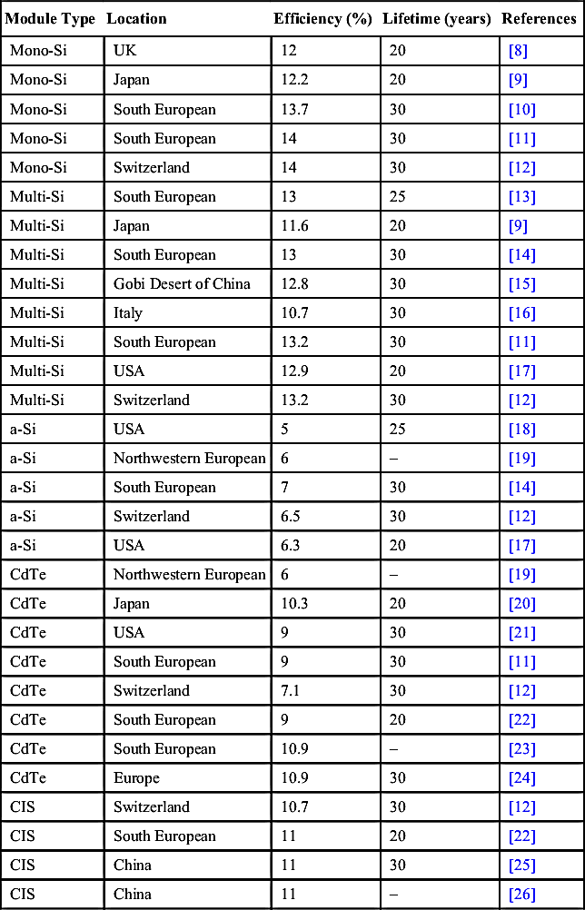
The variation of energy requirements is due to the variation in assumptions, energy mix, and manufacturing processes used in different studies. Most of the LCA studies found in the public domain are based on the LCA of mono-Si or multi-Si modules for power generation.

An LCA of a 4.2 kW_p standalone solar PV system was conducted in Spain by García-Valverde et al. [28]. The system considered in the study was a rooftop mono-Si solar PV system. Fig. 2.2 depicts the system boundary used in the study by García-Valverde et al. [28]. Transportation, supporting structure, and copper cables were also kept within the system boundary.

A similar kind of study was conducted by Kannan et al. [29] for Singapore. The authors considered a 2.7 kW_p grid-connected mono-Si solar PV system. On the other hand, Sumper et al. [30] assessed a 200 kW rooftop PV system with polycrystalline silicon modules for Catalonia, Spain. The same methodology (according to LCA framework) was used in these studies. There is very limited data for the energy consumption in manufacturing the balance-of-system (BOS), such as battery, inverter, charge controller, cable, supporting structure, and other accessories. The energy consumptions for various components used in these studies are represented in Table 2.3.

Transportation and installation usually require very little amount of energy. It is very difficult to trace the amount of energy that is consumed for the installation purpose. Transportation energy requirement can be calculated using the transportation distance and the energy intensity (MJ/t-km) of transportation medium. The energy requirement of the system must be amortized over the lifetime of the individual components. The electricity production can be found experimentally over the total lifetime (i.e., 20 or 30 years) of the PV plant. Also the amount of electricity generation can be calculated using Eq. (2.3), where El (kWh) is the amount of electricity produced throughout the plant's life, E (kWh/m²/year) is the amount of solar radiation received by the selected location,

η_{p}

$η_{p}$

and

η_{e}

$η_{e}$

are the efficiencies of the PV modules and inverter, respectively, A (m²) is the total area covered by the modules, and L (year) is the total lifetime of the PV system:

Table 2.2

The Range of Energy Requirements (MJ/m²) to Manufacture Various Solar Photovoltaic Modules

Module Type	Mono-Si	Multi-Si	a-Si	CIS	CdTe
Energy requirement (MJ/m²)	2860–5253	2699–5150	710–1990	1069–1684	790–1803

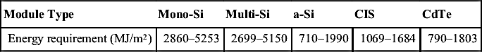
Adapted from Peng J, Lu L, Yang H. Review on life cycle assessment of energy payback and greenhouse gas emission of solar photovoltaic systems. Renewable and Sustainable Energy Reviews 2013;19:255–74.

Figure 2.2 Life cycle assessment system boundary. Adapted from García-Valverde R, Miguel C, Martínez-Béjar R, Urbina A. Life cycle assessment study of a 4.2 kW p stand-alone photovoltaic system. Solar Energy 2009;83:1434–45.

Table 2.3

The Energy Consumption for Various Components Used in the Earlier Studies in Literature

Component	García-Valverde et al. [28]	Kannan et al. [29]	Sumper et al. [30]
Photovoltaic module	1.583 MWh_th/m²^a	16 MWh_th/kW_p	4.59 × 10⁶ MJ
Al module frame	41.7 kWh_th/kg^b, 2.08 kWh_th/kg^c	Value taken from GEMIS^g	–
Charge regulator	277 kWh_th/kW_el	–	10.96 × 10⁴ MJ^h
Inverter	277 kWh_th/kW_el	0.17 MWh_el/kW_p	3.02 × 10⁴ MJ
Lead-acid battery	331 kWh_th/kWh^b, 242 kWh_th/kWh^c^,^d	–	–
Supporting structure	9.72 kWh_th/kg^b, 2.5 kWh_th/kg^c^,^e	Value taken from GEMIS^g	–
Cables	19.44 kWh_th/kg^b, 13.9 kWh_th/kg^c^,^f	–	–

$El = E \times η_{p} \times η_{e} \times A \times L$ $El = E \times η_{p} \times η_{e} \times A \times L$

(2.3)

The energy consumption is multiplied with the emission factors to get GHG emissions. Thermal energy can be converted to electrical energy with a thermoelectric conversion efficiency of 35% [28]. Table 2.4 represents the emission factors (EF) used in the study by García-Valverde et al. [28].

2.2.2. Life Cycle Assessment Results of Solar Photovoltaic System

The energy consumption, EPBT, and GHG emission are very much specific to the location under study. There is a wide range of these performance indicators observed among the studies in the public domain. The EPBT and GHG emission obtained from different studies are furnished in Table 2.5.

Table 2.4

Emission Factors for the Elements Used in the Solar Photovoltaic System

Component	Production From New Materials	Production From Recycled Materials	Recycling Process
Multi-Si module	93.6 g-CO₂/kWh_th	–	–
Al frame	14.6 kg-CO₂/kg	0.73 kg-CO₂/kg	0.73 kg-CO₂/kg
Charge regulator	93.6 g-CO₂/kWh_th	–	–
Inverter	93.6 g-CO₂/kWh_th	–	–
Lead-acid battery	93.6 g-CO₂/kWh_th	93.6 g-CO₂/kWh_th	0.16 g-CO₂/kg
Supporting structure	2.82 kg-CO₂/kg	0.45 kg-CO₂/kg	0.45 kg-CO₂/kg
Cable	5.57 kg-CO₂/kg	3.98 kg-CO₂/kg	3.98 kg-CO₂/kg

Adapted from García-Valverde R, Miguel C, Martínez-Béjar R, Urbina A. Life cycle assessment study of a 4.2 kW p stand-alone photovoltaic system. Solar Energy 2009;83:1434–45.

Table 2.5

Life Cycle Assessment Results Obtained From Different Studies

Module Type	Location	EPBT (years)	GHG Emissions (g-CO₂eq/kWh)	References
Mono-Si	UK	7.4–12.1	–	[8]
Mono-Si	Japan	8.9	61	[9]
Mono-Si	South European	2.6	41	[10]
Mono-Si	South European	2.1	35	[11]
Mono-Si	Switzerland	3.3	–	[12]
Multi-Si	South European	2.7	–	[13]
Multi-Si	Japan	2.4	20	[9]
Multi-Si	South European	3.2	60	[14]
Multi-Si	Gobi Desert of China	1.7	12	[15]
Multi-Si	Italy	3.3	–	[16]
Multi-Si	South European	1.9	32	[11]
Multi-Si	USA	2.1	72.4	[17]
Multi-Si	Switzerland	2.9	–	[12]
a-Si	USA	3	–	[18]
a-Si	Northwestern European	3.2	–	[19]
a-Si	South European	2.7	50	[14]
a-Si	Switzerland	3.1	–	[12]
a-Si	USA	3.2	34.3	[17]
CdTe	Northwestern European	3.2	–	[19]
CdTe	Japan	1.7	14	[20]
CdTe	USA	1.2	23.6	[21]
CdTe	South European	1.1	25	[11]
CdTe	Switzerland	2.5	–	[12]
CdTe	South European	1.5	48	[22]
CdTe	South European	0.79	18	[23]
CdTe	Europe	0.7–1.1	19–30	[24]
CIS	Switzerland	2.9	–	[12]
CIS	South European	2.8	95	[22]
CIS	China	1.6	10.5	[25]
CIS	China	1.8	46	[26]

Figure 2.3 Breakdown of CO₂ emission in a 4.2 kW_p stand-alone photovoltaic (PV) facility in the southeast of Spain. Adapted from García-Valverde R, Miguel C, Martínez-Béjar R, Urbina A. Life cycle assessment study of a 4.2 kW p stand-alone photovoltaic system. Solar Energy 2009;83:1434–45.

Most of the emissions come from manufacturing of lead–acid batteries (45%), followed by PV modules (39%). The breakdown of CO₂ emission is depicted in Fig. 2.3. Transportation, recycling, cables, and supporting structure together contribute about 10% CO₂ emission.

The reported values of EPBT and GHG emissions (see Table 2.5) of different PV systems vary significantly among the studies due to the variation of the influencing factors—PV module type, cell manufacturing technologies, installation methods, locations, weather conditions, and so on. Therefore, it is very important to conduct a location-specific LCA of a solar PV system.

2.3. Life Cycle Assessment of Wind Energy System

2.3.1. Methodology

In the present world, wind energy is becoming more and more popular for power generation in the areas where wind speed is sufficient for electricity generation. Several studies conducted LCAs of different capacity wind turbines around the globe. Tremeac and Meunier [31] assessed the environmental impacts of 4.5 MW and 250 W wind turbines. All the life cycle stages—manufacturing, transports, installation, maintenance, disassembly, and disposal—were considered in the study. The system boundary used for the study is depicted in Fig. 2.4. EPBT and CO₂ emissions were calculated, and it was found that wind energy can provide excellent environmental solution.

The functional unit used in most of the studies is kWh of electricity. GHG emissions are presented in the unit of g-CO₂eq/kWh_el. The main components of wind turbine systems are rotor, nacelle, tower, foundation, and grid connection cables. Guezuraga et al. [32] conducted an LCA of two different types of wind turbines with a lifetime of 20 years. The authors reported the material requirements for different parts of a wind turbine system. Table 2.6 represents the material requirements for a 1.8 MW gearless and a 2 MW geared wind turbines, respectively.

Figure 2.4 Life cycle assessment system boundary for wind turbine power generation. Adapted from Tremeac B, Meunier F. Life cycle analysis of 4.5 MW and 250 W wind turbines. Renewable and Sustainable Energy Reviews 2009;13:2104–10.

The recycling and waste disposal rates of different materials are furnished in Table 2.7. The recycling rates are very high for steel, cast iron, and copper that lead to lesser energy consumption.

The operational phase hardly requires any energy consumption. The energy requirements in the transportation of wind turbine parts to the wind site can be calculated using the transportation distance and energy intensity of modes of transportation used. The energy consumption in transportation of raw materials to the manufacturing plants can be ignored as it is very difficult to trace [33].

A wind turbine is used to convert the kinetic energy of wind into mechanical power. The rotating shaft is coupled with the generator, which converts the mechanical power into electrical power. The electricity provided by a wind turbine can be AC or DC. The amount of effective mechanical power can be estimated using Eq. (2.4), where P (W) is the mechanical power generated, c_p (%) is the capacity factor, ρ (kg/m³) is the density of air, A (m²) swept area of the blades, and V (m/s) is the average wind velocity:

$P = \frac{1}{2} c_{p} {ρAV}^{3}$ $P = \frac{1}{2} c_{p} {ρAV}^{3}$

(2.4)

The electrical energy delivered by the turbine throughout the lifetime can be found from the power developed, generator efficiency, and operation hours of the turbine per year, and the lifetime of the wind turbine (i.e., 20 years).

2.3.2. Life Cycle Assessment Results of Power Generation From Wind

The primary energy consumption and emission factors for manufacturing various materials used in wind turbines and for recycling and landfilling are presented in Table 2.8. According to Guezuraga et al. [32], most of the energy is consumed in the manufacturing phase, which is 84.4%, followed by transportation (7%) and maintenance (4.3%), respectively. Fig. 2.5 represents the breakdown of energy consumption in different stages of a wind turbine power plant.

Table 2.6

Material Requirements for the 1.8 MW Gearless and 2 MW Geared Turbines

Material	1.8 MW Gearless Turbine		2 MW Geared Turbine^a
Material	Mass (tonnes)	Wt. (%)	Mass (tonnes)	Wt. (%)
Stainless steel	178.4	29.9	296.4	19.3
Cast iron	44.10	5.9	39.35	2.6
Copper	9.90	1.6	2.40	0.2
Epoxy	4.80	1.8	10	0.6
Plastic	1.85	0.3	2.40	0.2
Fiberglass	10.20	2.6	24.30	1.6
Reinforced concrete	360	57.9	1164	75.6

Table 2.7

Recycling and Waste Disposal Rates of Different Materials

Material	Type of Dismantling
Stainless steel	90% recycle, 10% landfill
Cast iron	90% recycle, 10% landfill
Copper	90% recycle, 10% landfill
Epoxy	100% incinerated
Plastic	100% incinerated
Fiberglass	100% incinerated
Concrete	100% landfill

Adapted from Guezuraga B, Zauner R, Pölz W. Life cycle assessment of two different 2 MW class wind turbines. Renewable Energy 2012;37:37–44.

It was observed that material manufacturing and transportation are the unit processes that mostly affect the life cycle energy and resulting GHG emissions. Table 2.9 shows a country-specific overview of energy and CO₂ analysis of wind turbines.

The reported values of energy intensity and emissions (see Table 2.9) of different capacity wind turbines vary significantly among the studies due to the variation of different influencing factors—turbine manufacturing technologies, wind speed, energy mix of the location, and so on. Hence, it is very important to conduct a location-specific LCA of a wind turbine electricity generation system.

Table 2.8

Embodied Energy and Emission Factors for Different Materials, Recycling, and Landfilling

Material	Energy Requirements (GJ/tonnes)	GHG Emissions (kg/tonnes)
Material	Energy Requirements (GJ/tonnes)	CO₂	CH₄	N₂O
Material Production
Steel	34	2473	0.04	0.07
Stainless steel	53	3275	0.04	0.07
Rebar steel	34.26	2163.83	0.10	0.07
Glass	8.70	566	0.04	0.01
Epoxy	45.70	3941	0.04	0.12
Polyester	45.70	3941	0.08	0.12
Copper	78.20	6536	0.16	0.19
Aluminum	39.15	3433.50	0.07	0.11
Concrete	0.81	119.02	0.03	8.7E-5
Material Recycling		Kg-CO₂eq/tonnes
Steel	9.70	1819
Aluminum	16.80	738
Copper	6.40	3431
Landfilling operations	0.04	0.90

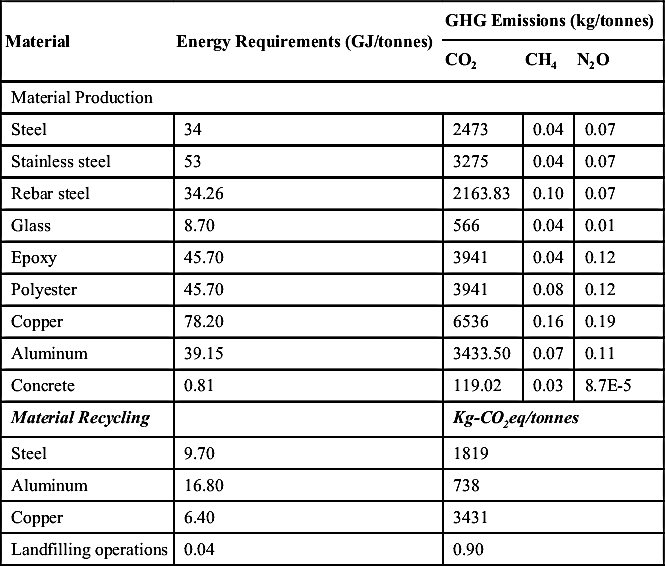
Adapted from Kabir MR, Rooke B, Dassanayake GM, Fleck BA. Comparative life cycle energy, emission, and economic analysis of 100 kW nameplate wind power generation. Renewable Energy 2012;37:133–41.

Figure 2.5 Breakdown of the total life cycle energy requirements. Adapted from Guezuraga B, Zauner R, Pölz W. Life cycle assessment of two different 2 MW class wind turbines. Renewable Energy 2012;37:37–44.

Table 2.9

The Energy Intensity and Emissions of Different Wind Turbine Plants Around the Globe

Power Rating (kW)	Location	Energy Intensity (kWh/kWh)	Emissions (g-CO₂/kWh)	References
30	Denmark	0.1	–	[34]
100	Japan	0.456	123.7	[35]
500	Brazil	0.069	–	[36]
1500	India	0.032	–	[37]
6600	UK	–	25	[38]
100	Japan	0.16	39.4	[39]
300	Japan	–	29.5	[40]
3	USA	1.016	–	[41]
10 × 500^a	Denmark	–	16.5	[42]
18 × 500^b	Denmark	–	9.7	[42]
30–800	Switzerland	–	11	[43]
1.8 and 2	Austria	–	9	[32]^c
5, 20, and 100	Canada	–	(42.7, 25.1, and 17.8)^d	[33]^e

2.4. Life Cycle Assessment of Biofuels

Biofuels are one of the oldest fuels in place. From time immemorial, wood and straw have been used as fuel for various purposes, which suited the time. With the industrial revolution, however, the need for concentrated source of energy pushed biofuels on the margin and welcomed the use of fossil fuels. In the late 20th and 21st centuries, however, the problems of global warming and other environmental abuse have ushered a renewed interest in renewable energy and thus in biofuels as well. A proof of that is, since 2000s there has been a marked increase in the production of bioethanol. It rose from 16.9 billion liters in 2000 to 72 billion liters in 2009 [44]. In Poland, it is expected that there will be a sharp rise in production of bioelectricity from 2010 to 2030. Electricity production from solid biomass will increase from 5.5 to 11.1 TWh/year in Poland [45]. Although biomass has a distinct advantage of being deemed as carbon neutral, it comes with caveats, such as “food versus fuel” debate and consequences related to land use [46]. To identify savings in energy and emissions from biofuel production, its utilization, and its corresponding environmental effects, a thorough evaluation of the corresponding life cycle is to be carried out carefully. LCA is an effective tool for this as it can unravel and quantify the potential environmental impacts and evaluate the inputs and outputs [5].

It should be noted that a striking feature of LCA for biofuel is that it gives differing results, and thus a range of results is obtained for even the same fuel as illustrated in Fig. 2.6. These differences can be attributed to different types of feedstock sources, conversion technologies, end-use technologies, system boundaries, and reference energy system. Also, region plays a significant part in LCA and so does the development of fuel conversion technology [47,48]. Despite this, it can be said with confidence that most biofuel-based LCA shows a reduction of GHG emission when used as a substitute or in combination with fossil fuel in transportation sector [49–51]. In the environmental aspect, such as land use or eutrophication, however, majority of studies shows that biofuel have negative impacts when aimed to reduce the GHGs [49,52,53]. Thus, making a decision regarding the use of biofuels is sometimes as black and white as deemed.

Figure 2.6 Well to wheel (WTW) energy requirements and greenhouse gas emissions for conventional biofuel pathways compared with gasoline and diesel pathways showing the range of life cycle assessment results of biofuels [49].

This section of the review seeks to discuss briefly the findings regarding the first- and second-generation biofuels and their implications. The aim of this section is to summarize the key LCA issues influencing outcomes for bioenergy and to provide an overview of the GHG and energy balances of the most relevant bioenergy chains in comparison with fossil fuels.

2.4.1. Biomass Source

When including both the first- and the second-generation biofuels, the source of biomass covers a wide range. A basic definition for biomass is that it is renewable organic matter that includes plant and animal products and excretions, food processing and forestry by-product, and urban waste [54]. The first-generation biofuels are derived from the parts that are or can also be used as food materials for humans, while the second generation uses lignocellulosic parts of the biomass. Hence bioethanol derived from sugarcane or rapeseed is first-generation biofuel, while from Jatropha or wood would be second generation. In LCA study, the biomass supply plays a key role since the source has a big impact on the LCA outcome. The biomass supply can be divided into two main categories: residues and energy crop.

Biomass residues and waste are not specifically produced as energy resource, but are by-products from agriculture, forestry, households, and so on. Most of these biomass and residues are inevitable in any economic activity or industrial process [55]. Due to this aspect, its use in making biofuels usually does not adversely affect the environment; although there is some backlash, since there is already a system established in nature and displacing something would hamper it. For example, the removal of agriculture by-products hampers the carbon cycle by reducing the carbon storage in the soil. Not to mention the use of such residue could potentially invite a more thorough use of the parent mechanism and thus could cause some permanent damage to the ecosystem, such as deforestation.

Energy crops, on the other hand, are cultivated with the intent to provide a feedstock for biofuel development [56]. Those feedstocks generated from agricultural activities and forest log can be included in this as well [57]. To avoid excess environmental burden related to agricultural chain, the types of energy crops grown are suggested to use high-yielding species [57], which would require minimal maintenance [58] and can survive in marginal or degraded lands. While it is difficult to find a crop that meets all these criteria, perennial C4 grasses, such as Miscanthus and switchgrass (Panicum virgatum L.), are particularly promising [59]. Excessive cultivation of such crops can lead to some problems such as deforestation, directly for its cultivation or indirectly by displacing a nonenergy crop, and also eutrophication due to the use of fertilizers and pesticides. However, cultivation of energy crops also has the added benefit of providing certain ecosystem services, such as C-sequestration, increase in biodiversity, salinity mitigation, and enhancement of soil and water quality. It should be noted that to be accepted as an energy crop, it must fall within the parameters of sustainable agriculture.

A typical form of biofuel source is manure and if not treated well, which may be the case in developing countries, the effect is quite damaging to the environment. In China, it is estimated that poultry and livestock manure reached about 3.97 × 10⁹ tons in 2007, majority of which was drained into the river resulting in water pollution and GHG emissions. In countries with these problems, biogas production from manures is a sound solution both for the environment and for electricity production [60].

2.4.2. Methodology

LCA is a structured approach to analyze a system and thus it follows a particular strand of approach. It seeks to incorporate the environmental and economic impacts of all the stages in a production chain and removes ambiguities thereby giving a holistic picture of a system. This section will give a general idea of the methodology of LCA and will give an idea of how biofuels fit into this methodology.

2.4.2.1. Goal, System Boundaries, and Functional Unit

The first step involves in defining the goal and scope, which defines the purpose, audiences, and system boundaries. Since this process will be a controller for the rest to come, it has to be very specific in detailing what to include and what to exclude thereby creating an analysis system boundary. It can simply include the GHG emission, and thus the study will be centered around the direct and indirect emissions during the formation of the biofuel. It can also exclude the GHG and concentrate on the environmental impacts in which case the LCA would collect, assess, and interpret the data obtained regarding issues, such as eutrophication, acidification, biodiversity change, and so on.

The functional unit is defined as the quantification of the identified performance characteristics of the products [5]. It gives a reference to which the input and output data are normalized and harmonizes the establishment of the inventory. This also provides a means for comparison among different LCA studies provided that the system boundaries are similar. It should be noted that different functional units for the same LCA will give different outcomes, and hence it is imperative to choose the one that satisfies the goals of LCA the best. For example, to study the effect biofuels have on the transportation sector, the most comprehensive functional unit is to record the effect (e.g., GHG emission) by vehicle-km basis [49]. If the goal is to ensure the optimum use of land while using energy crops as the biomass supply, a useful way would be to represent the results on a per hectare basis [61]. In order to be independent from the kind of feedstock, the results should be expressed in per unit output, for example, kWh, and should be expressed in per unit input, for example, kg, in order to be independent of the conversion process.

To illustrate the method described, here is an example where both the goal scope and the functional unit are clearly specified. It is taken from the study that develops an LCA for the generation of bioelectricity [62] and is as follows: “The aim of this study is to evaluate the contribution to CO₂ emission reduction that can be achieved by means of using biomass for energy production, in comparison with conventional fuel use. The functional unit is the produced energy unit (1 MJ), to which inventory data and results are referred to.”

2.4.2.2. Life Cycle Inventory Analysis

In this process, for each unit of input and output of energy, mass flows and emission data are collected, validated, and categorized. The system boundary plays a very important role in this part since it dictates what data to incorporate and what to reject. Something indirectly important to the LCA might not even be applicable. For example, a study by Wiloso et al. [63] documents that out of 25 studies that use enzymatic action in processing lignocellulosic biomass, only 15 incorporated enzyme production in their inventory analysis. To further illustrate the life cycle inventory (LCI) analysis, Fig. 2.7 adapted from a study by Corti and Lombardi [62] is presented.

2.4.2.3. Allocation Methods

Allocation is a process of attributing environmental burden of multifunctional process to only those functions that are associated with it [64]. It is, however, to be avoided if possible either through the division of the whole process into subprocesses related to coproducts or by expanding the system boundaries (substitution approach) to include the additional functions related to them [5]. If not avoided, then the question of which method to use and what numerical values to be used is raised. And depending on the method of allocation to the coproduct or the source technology, the LCA values can change significantly. For example, in a case study where bioethanol is produced from wheat, the output differs significantly as shown in Fig. 2.8.

In Fig. 2.8, different models represent different means by which the power was obtained for the conversion process in the LCA. The description of each model is given in Table 2.10.

Figure 2.7 An example of life cycle inventory.

Figure 2.8 Variations in CO₂ output due to source allocation [65].

Table 2.10

Model Description Used in the Study Conducted by Punter et al. [65]

Model	Description
a	Conventional natural gas–fired steam boiler + imported electricity
b1	Conventional natural gas–fired steam boiler + backpressure steam turbo-generator
b21	Natural gas–fired gas turbine + unfired HRSG + backpressure steam turbo-generator
b22	Natural gas–fired gas turbine + cofired HRSG + backpressure steam turbo-generator
c1	Straw–fired steam boiler + backpressure steam turbo-generator
c2	Straw–fired steam boiler + backpressure and condensing steam turbo-generator

Table 2.11 adapted from a study by Singh et al. [66] shows different allocation methods for the production of bioethanol.

2.4.2.4. Impact Assessment

Impact assessment creates a connection between the product or process and its potential impacts on human health, environment, and source depletion. The impact assessment requires categorizing the effect of the biofuel production. It mainly looks into whether or not systems give surplus energy, followed by concern on global warming, eutrophication, acidification, water and land use, and so on. For example, it has been suggested that biofuels based on Jatropha are appropriate for small-scale, community-based production aimed at local use [52,67]. In the study by Corti and Lombardi [62], the category for impact assessment is kg of equivalent CO₂ per functional unit (MJ). This is because as the goal stated the aim was to evaluate the contribution of CO₂ emission reduction during the harvesting of bioenergy. Thus the goal and scope, and functional unit matter when it comes to defining the impact category.

Table 2.11

Biomass and Its Reported Allocation Methods

Biomass	Allocation Method
Maize (grain)	Displacement, replacement, system expansion, Economy value energy content of outputs, mass, subdivision
Maize (stover)	System expansion, substitution, mass
Cellulose	System expansion, displacement
Sugarbeet and wheat (grain)	System expansion, mass, energy, market value
Sugarcane	None

2.4.3. Energy Balance, Greenhouse Gas Emission, and Environmental Concerns

2.4.3.1. Energy Balance

Usually, net energy value (NEV) is used in studying the issue of energy surplus. It is basically an efficiency term calculated by taking the difference between the usable energy produced from a biofuel crop and the amount of energy required in the production of that fuel for energy. A negative NEV indicates energy loss; that is, more energy is required to produce the biofuel than the amount of energy that can be used for fuel. A positive NEV is an estimate of the energy gained for fuel use in the production process indicating surplus of energy.

However, this categorization has an obvious flaw; that is, NEV calculation is too simplistic and gives a raw energy output, but not all forms of energy are the same. Different forms incur different costs and benefits. In reality, the service gained from fuel energy matters mostly. Therefore, it might be more accurate to compare biofuel energy balance directly to the fossil fuel energy equivalent that can be displaced. This is generally reported as a ratio of the amount of energy produced to the amount of fossil fuel energy required to produce it. This new term is called fuel energy ratio (FER). An FER < 1 indicates net energy loss, while an FER > 1 indicates a surplus of energy. Table 2.12 adapted from a study by Davis et al. [68] shows the FER for different crops.

2.4.3.2. Greenhouse Gas Emission

Since biomass as fuel is relatively recent when compared to fossil fuels, which are locked below the earth for thousands of years, burning the former is considered to be carbon neutral. This comes from the assumption that it burns off the same amount of carbon dioxide that it consumed throughout its life, which is relatively short. This entails that bioenergy has an almost closed CO₂ cycle. This though sounds perfect presents us with a hidden caveat that there are GHG emissions in its life cycle largely from the production stages where fossil fuel inputs are required to produce and harvest the feedstocks, in processing and handling the biomass, in converting the biomass to fuel, and in transporting the feedstocks and biofuels.

Table 2.12

Estimated Fuel Energy Ratio (FER) Values of Some Biofuel Crops

Biofuel Crop	FER
Corn	1.95
	1.76
	1.67
	1.64
	1.62
	1.60
	1.52
	1.51
	1.39
	1.34
	1.32
	1.28
	1.27
	1.25
	1.22
	1.21
	1.08
	0.99
	0.95
	0.92
	0.8
	0.78
	0.69
Lignocellulosic crops (generalized)	5.6
	4.3
	3.51
	2.62
	2.19
	1.8
Miscanthus (combustion)	1.16
Miscanthus (gasification)	0.99
Switchgrass	4.43
Switchgrass	0.44

The most uncertain greenhouse gas in the biofuel life cycle is nitrous oxide (N₂O). It evolves from the decomposition of organic matter and from the application of fertilizers [69]. Since fertilization rates are higher for annual crops than for perennial energy crops, N₂O emission is higher in those. Crops grown in high rainfall environments or under flood irrigation have particularly high N₂O emissions, as denitrification, the major process leading to N₂O production, is favored under moist soil conditions where oxygen availability is low. As the emission of N₂O lacks a point source, the estimation of its emission is very difficult [70]. This uncertainty is even more magnified since the GWP of the N₂O is very high around 298 times as that of CO₂ [49].

Methane (CH₄) is the last major emission in the life cycle after CO₂ and N₂O. This is released by anaerobic decomposition of organic feedstocks or by reducing the oxidation of the soil thereby reducing the methane content in it while releasing it into the atmosphere. Its GWP is 23 times as that of CO₂, thus considerably lower than that of N₂O.

The most pertinent GHGs mentioned earlier; that is, CO₂, CH₄, and N₂O, are called direct GHGs since they impact the climate directly. Other gases that are emitted throughout the life cycle are carbon monoxide (CO), nonmethane organic compound (NMOC), and ozone (O₃) [49]. In order to take a holistic look into the GHG emissions, both the emissions need to be accounted for and all of the emissions are to be converted to the carbon dioxide equivalents. Taking all of the direct and indirect emissions, sometimes it may so happen that a particular brand of biofuel emits more GHGs than the conventional fuel. Thus a blanket statement regarding the GHG emission is not possible. Fig. 2.9 shows the GHG emission in CO₂ equivalents for different biofuels. It has been adapted from the study by Fritsche and Hennenberg [71], and it gives the maximum and minimum values for all the biofuels given. From Fig. 2.9, it can be noted that some fuels have higher GHG emission than conventional diesel and gasoline.

The study by Corti and Lombardi [62] gives comparative results of the equivalent CO₂ emission per MJ of electricity produced for both biofuels-based and coal-based electricity production. The results are adapted to graphical format (Fig. 2.10 for biomass-based electricity and Fig. 2.11 for coal-based electricity) for comparative purpose.

2.4.3.3. Land Use and Other Environmental Issues

The land use for biomass can be divided into direct land use and indirect land use. Direct land use is when biofuel feedstock is cultivated in a land already in use for something. Thus, if there was a forest or any other kind of agriculture, such as rice, wheat, and so on, and it was displaced to grow sugarcane or sunflower for biofuel, then that would be direct land use. Such land use can bring issues, such as change in indigenous carbon cycle. It necessarily is not bad since whether or not the soil carbon content increases depends on the biomass feedstock crop and the previous crop/plantation.

Indirect land use is the term used to describe the phenomena that occurs when the biofuel feedstock occupies a land already in use forcing the previous plantations to occupy another land. This could happen if the production demand for the previous land use still exists; for example, in the case of crops such as rice or wheat, and thus these are cultivated in another land which may prompt unfavorable land use change [71].

Figure 2.9 Life cycle GHG emissions of different biofuels and conventional gasoline and diesel including indirect land use change. Adapted from Fritsche UR, Hennenberg K. The “iLUC Factor” as a means to hedge risks of GHG emissions from indirect land-use change associated with bioenergy feedstock provision. In: Background paper for the EEA expert meeting in Copenhagen, 2008.

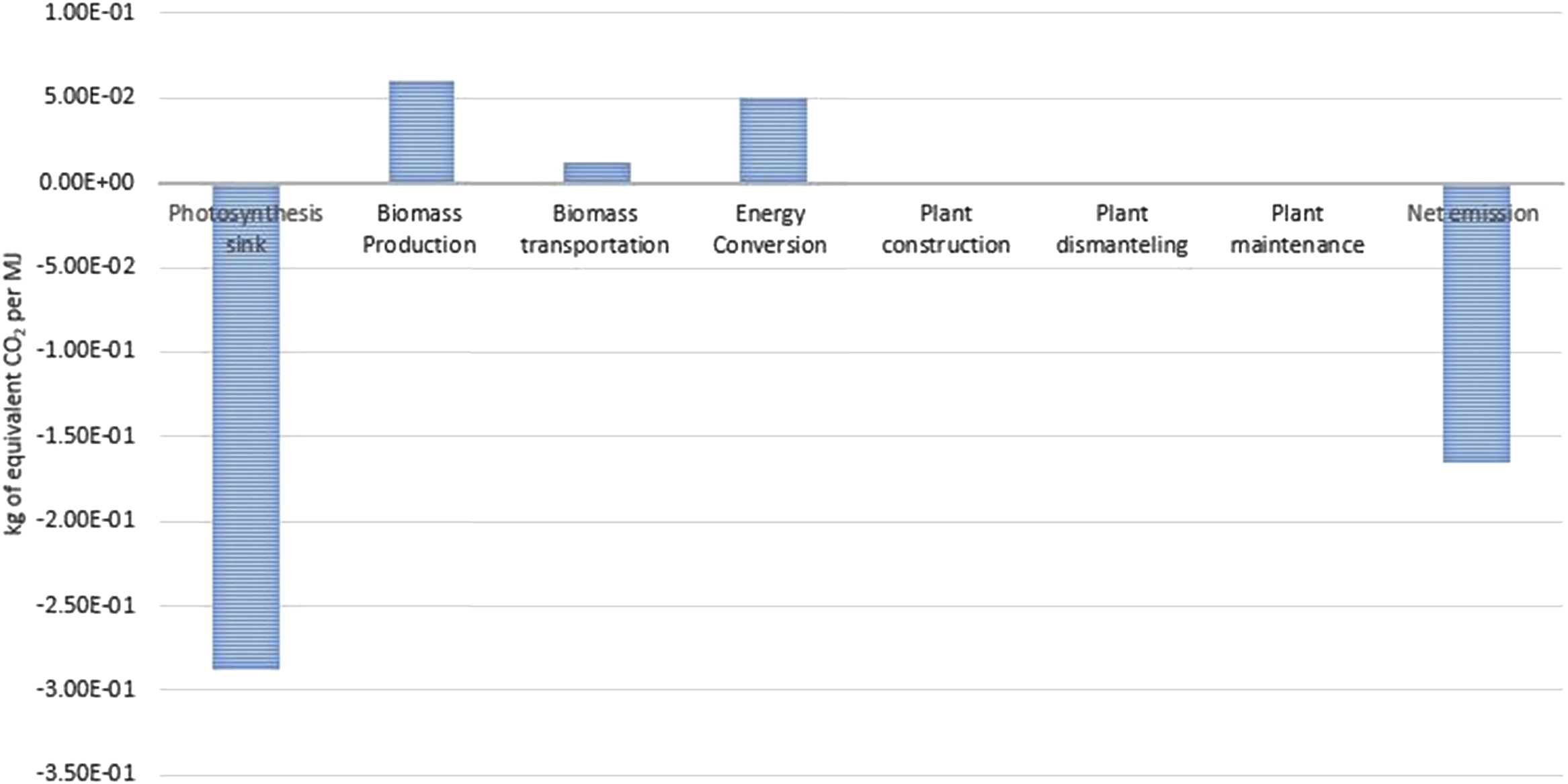
Figure 2.10 Illustration of kg of CO₂ equivalents per MJ for biomass-based electricity production [62].

Excessive land use causes little pertinent damage to the environment since the land is used to grow crops and that comes with a baggage of other needs, such as fertilizers and pesticides. Use of such may increase the risk of eutrophication and acidification if it is washed away into local water bodies or seeps into ground water. Although in the case of biogas production, which is mainly a product of anaerobic action on manure, in some cases it can elevate the environmental condition if the manure is released into the environment untreated otherwise [60]. One way to note the damage is to define the impact categories meticulously, a categorization is Eco-Indicator 99 methodology which includes the impact categories into three types of damage: “Damage to human health,” which includes the following impacts: carcinogenesis, organic respiratory effects, inorganic respiratory effects, climate change, ionizing radiation, and reduction of the ozone layer; “damage to ecosystem quality,” which includes ecotoxicity, acidification/eutrophication, and land use; and “resource damage,” which includes minerals and fossil fuels [72].

Figure 2.11 Illustration of kg of CO₂ equivalent per MJ for coal-based electricity production [62].

In the study conducted to analyze the production of biofuels from different vegetable oils [72], it is noted that the production of soybean has an impact of 70% in the category of carcinogens, 34.3% in the category of respiratory inorganics, 55% in the category of acidification and eutrophication, and 35.5% in the category of land use. If the impact categories are normalized to show how much each factor, noted in Eco-Indicator 99, is effected compared to each other, the result showed in Fig. 2.12 is obtained.

Thus, from the study it can be readily concluded that apart from climate change, the culturing of biofuel feedstocks and making biofuels have adverse effect on the environment. Thus making biofuels more ubiquitous is a double-edged sword. One needs to make a balance between the environmental degradation in comparison to the net reduction of GHGs into the atmosphere. There is no universal right choice regarding what to do, rather it is always case specific.

Figure 2.12 Normalization of the environmental burdens by impact category [72].

2.4.4. Reasons for Uncertainties in Biofuel Life Cycle Assessment

It should be obvious by now that LCA of biofuels results in somewhat ambiguous results, and sometimes one data contradicts the other. It is best illustrated in Table 2.12 where corn gives both FER > 1 and FER < 1. Also it can be seen in Fig. 2.9 where some fuel range shows the emission can be both lower and greater than conventional diesel and gasoline. This feature of LCA results partly from the myriads of uncertainties that creep into the analysis throughout its working and partly from the fact that there are wide range of plausible values for key input parameters with values often dependent on local condition. Same feed materials and output can have more than one path to follow. For example, a study by Wiloso et al. [63] notes that using lignocellulose as feed to obtain bioethanol can be done in two ways. The widespread one is to hydrolyze the biomass feedstock and then ferment it; however, it can also be done by gasifying the feed to form syngas and then either fermenting it or using a catalyst to convert it to ethanol. Now even with the fact that the product and the feed were the same, the path undertaken was different and as shown before, the path taken to produce will have an effect on the final outcome of the LCA. Also land use and technology use differ from place to place and time to time and thus LCA outputs vary from time and place.

Keeping these reasons aside, Larson provides four basic reasons why there are such major uncertainties [49] (All of these reasons are discussed in brief in this discussion and hence not repeated):

1. the climate-active species included in the calculation of equivalent GHG emissions (Section 2.4.3.2);

2. assumptions around N₂O emissions (Section 2.4.3.2);

3. the allocation method used for coproduct credits (Section 2.4.2.3);

4. soil carbon dynamics (Section 2.4.3.3).

From this study, it should be obvious that biofuels are not a door to utopia. It has its fair share of problems, which can be a major issue if not regulated. Biofuels are shown to lower the overall GHG into the atmosphere if the right one is chosen. However, in doing so it introduces major environmental degradation. Thus, to make a choice to move toward biofuels must be an educated one, which accounts for the consequence and is prepared to offset it thereby making the fuel truly sustainable.

2.5. Life Cycle Assessment of Biogas

Biogas is a fuel gas produced from biomass and/or from the biodegradable fraction of wastes, which can be purified to natural gas quality, to be used as biofuel. The gas consists mostly of CH₄ and CO₂ and is produced from the bacterial anaerobic action on the feedstock. Fig. 2.13 shows the typical composition of biogas.

Electricity from biogas concept is on the rise especially for European countries as the GHG emission needs to be curbed to favorable level. In Poland it has been estimated that electricity from biogas is expected to rise from 0.4 to 6.6 TWh/year from 2010 to 2030. Also, bioelectricity provides a huge economical potential as it has been estimated that it can provide almost 30% of energy demand in China [45]. Also the quantity of small-scale biogas digesters has increased from about 1.8 × 10⁹ m³ in 1996 to 1.0 × 10¹⁰ m³ in 2007, while the number of large- and medium-scale biogas projects has increased from about 1.2 × 10¹¹ m³ in 1996 to 6.0 × 10¹² m³ in 2007.

Figure 2.13 Composition of biogas. Adapted from A Biogas Road Map for Europe. European Biomass Association 2010, https://www.americanbiogascouncil.org/pdf/euBiogasRoadmap.pdf.

2.5.1. Feedstock and Environmental Effects

The feedstock of biogas is not limited to a single biomass source. However, the waste and manure is the most obvious source for biogas. Thus, it is sometimes a surprise to know that even the herbaceous materials can and do contribute to the formation of biofuels. Fig. 2.14 shows the list of sources and its use along with the percentage of methane that is formed from those sources.

The environmental effects of biomass use have already been briefed in Section 2.4.3.3; however, in the case of biogas since waste and animal discharge plays a big part, there is an added benefit. The environmental advantages of using sewage-derived biogas relate to the reduction of problematic sludge by about 50% (dry mass basis). Also, biogas that has methane, carbon dioxide, and hydrogen sulfide, which is toxic, is naturally released from wastes in landfills and its oxidation is necessary for prohibiting the release of methane and volatile organic compounds to the atmosphere thus improving local air quality [45].

2.5.2. Greenhouse Gas Emission and Electricity Production

The toxic emission of biogas combustion is relatively cleaner than petrol and diesel. This makes it a very attractive fuel. The relative reduction of toxic emission, which includes GHG, in comparison to petrol and diesel is given in Fig. 2.15.

However, the other side of the story is hinted in the study by Ishikawa et al. [75]. It documents the total equivalents of CO₂ emission in kg for a biogas plant in Betsukai, Hokkaido. The CO₂ emission for each item is given in Table 2.13.

Figure 2.14 Biogas yield for different biomass feedstock.

Figure 2.15 Reduction of toxic emissions in % from biomethane in comparison to petrol and diesel. Adapted from Rutz D, Janssen R. Biofuel technology handbook. Munich (Germany): WIP Renewable Energies; 2007.

Table 2.13

CO₂ Emissions of Biogas Plant in Hokkaido [75]

Items	CO₂ Emissions (kg)
Initial energy investment	2,589,000
Operating energy	78,000
Maintenance energy	–
Total	2,667,000

Budzianowski [45] notes and compares three ways of producing electricity from biomethane. First one is combustion of biomethane with air, the second one involves oxyfuel combustion of biomethane where the components other than oxygen in air are stripped out and pure oxygen is used instead of air for combustion. The third one is called oxy-reforming fuel cell (ORFC) where CH₄ is split into CO and H₂ in the oxygen stream atmosphere. The energy required for this splitting is obtained from the exothermic reaction as CO is converted to CO₂. The H₂ on the other hand is used in the H₂ fuel cells for production of electricity. The result after the comparison of the three mentioned method to produce electricity is given in Table 2.14.

Thus, it can be seen that electricity generation from biogas though viable has its issues as well. The environmental issues discussed in Section 2.4.3.3 still stands. It is a better form of fuel than the fossil fuels in use; however, there are some issues with GHG during the formation and operation of biogas plants. As stated before there is no choice that can lead to utopia. Every technology comes with its disadvantage. It is thus wise to know what they are to make prudent judgment regarding adapting any technology.

Table 2.14

Comparison Among Different Ways of Producing Electricity From Biogas

	Combustion	Oxyfuel Combustion	Oxy-Reforming Fuel Cell
Net electricity output (kJ/mol CH₄)	431.2	411.2	450.2
Net efficiency (%)	53	51	56

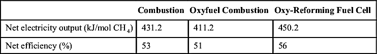
Adapted from Budzianowski WM. Can ‘negative net CO₂ emissions’ from decarbonised biogas-to-electricity contribute to solving Poland's carbon capture and sequestration dilemmas? Energy 2011;36:6318–25.

2.6. Life Cycle Assessment of Hydropower Plants

Hydropower is the major renewable electricity generation technology being used in 159 countries having advantages such as high level of reliability, high efficiency, proven technology, very low operating and maintenance cost, flexibility, and large storage capacity. It contributes to more than 16% of worldwide electricity generation and about 85% of global renewable electricity. International Energy Agency (IEA) roadmap on hydropower predicts a global capacity of 2000 GW resulting in over 7000 TWh of electricity by the year 2050. China, Brazil, Canada, and the United States together produce half the world's hydropower (Table 2.15). In 2010, 36 countries generated more than 50% of their total electricity from hydropower [76] (Table 2.16).

Hondo [40] has conducted a life cycle GHG emission analysis for a hydropower plant in Japan having a gross output of 10 MW with a capacity factor of 45%. The plant lifetime was considered to be 30 years. The plant analyzed was a run-of-the-river type with a small reservoir. The constituents of the plant are a small concrete dam (2000 m³ volume), a penstock (9000 m), a pressure pipe (490 m), and a powerhouse. The maximum intake to the powerhouse was 4.8 m³/s. Table 2.17 shows the life cycle GHG emission factors (LCEs) and their breakdowns for the hydropower plant studied.

Table 2.15

Top 10 Hydropower Producers in 2010 [76]

Country	Hydroelectricity (TWh)	Share of Electricity Generation (%)
China	694	14.8
Brazil	403	80.2
Canada	376	62.0
United States	328	7.6
Russia	165	15.7
India	132	13.1
Norway	122	95.3
Japan	85	7.8
Venezuela	84	68
Sweden	67	42.2

Table 2.16

Countries With More Than Half of Their Electricity Generation From Hydropower in 2010

Share of Hydropower	Countries
∼100%	Albania, DR of Congo, Mozambique, Nepal, Paraguay, Tajikistan, Zambia
>90%	Norway
>80%	Brazil, Ethiopia, Georgia, Kyrgyzstan, Namibia
>70%	Angola, Columbia, Costa Rica, Ghana, Myanmar, Venezuela
>60%	Austria, Cameroon, Canada, Congo, Iceland, Latvia, Peru, Tanzania, Togo
>50%	Croatia, Ecuador, Gabon, DPR of Korea, New Zealand, Switzerland, Uruguay, Zimbabwe

Adapted from International Energy Agency. Technology roadmap: hydropower, https://www.iea.org/publications/freepublications/publication/2012_Hydropower_Roadmap.pdf.

Table 2.17

Life Cycle GHG Emission Factors for Hydropower Plant Studied by Hondo [40]

	g-CO₂/kWh	Share (%)
Construction	9.3	82.8
Machinery	0.9	8.0
Dam	0.5	4.5
Penstock	4.5	39.8
Other foundations	2.4	21.0
Site construction	1.1	9.6
Operation	1.9	17.2
Total	11.3	100.00

The results suggest that 82.8% of CO₂ is emitted during construction as compared to 17.2% CO₂ emission during operation. The LCEs for hydropower plant depend prominently on the assumption of lifetime and capacity factor [40]. Tables 2.18 and 2.19 show the effect of lifetime and capacity factor on LCE (g-CO₂/kWh) for hydropower plant.

Pascale et al. [77] have conducted an LCA study of a 3 kW run-of-river community hydroelectric system located in Huai Kra Thing (HKT) village in rural Thailand. They have modeled the construction, operation, and the end-of-life phases of the hydropower plant over a period of 20 years. The model includes all the relevant equipment, materials, and transportation; 1 kWh of electrical energy has been considered as functional unit in the study. Fig. 2.16 shows the scope and system boundary of the study. Table 2.20 shows the results of the study in terms of GWP in g-CO₂/kWh [77].

Table 2.18

Effect of Lifetime on Life Cycle GHG Emission Factor for Hydropower Plant Studied by Hondo

Lifetime (years)	10	20	30	50	100
g-CO₂/kWh	30	16	11	8	5

Adapted from Hondo H. Life cycle GHG emission analysis of power generation systems: Japanese case. Energy 2005;30:2042–56.

Table 2.19

Effect of Capacity Factor on Life Cycle GHG Emission Factor for Hydropower Plant Studied by Hondo

Capacity factor	−10 pt	−5 pt	Reference	+5 pt	+10 pt
g-CO₂/kWh	14	13	11	10	9

Adapted from Hondo H. Life cycle GHG emission analysis of power generation systems: Japanese case. Energy 2005;30:2042–56.

Gallagher et al. [78] have calculated the environmental impacts of three (50–650 kW) run-of-river hydropower projects in the United Kingdom using the LCA tool. The GHG emissions from the projects to generate electricity ranged from 5.5 to 8.9 g-CO₂eq/kWh, which is very low as compared to 403 g-CO₂eq/kWh for UK marginal grid electricity. The system boundary considered for the study included raw material extraction, processing, transport, and all installation and grid connection operations. The functional unit was 1 kWh of electricity generated and the lifespan has been considered to be 50 years. Fig. 2.17 shows the system boundary used in the study. Table 2.21 shows the descriptions of three run-of-river hydropower plant case studies and their environmental impacts.

Figure 2.16 Schematic diagram of scope and system boundary used by Pascale et al. [77].

Table 2.20

Life Cycle Assessment Results for Different Components of the Hydropower Plant

	Weir, Intake, Canal and Forebay	Penstock	Powerhouse, Turbine, and Outflow	Transmission Line	Control House and Control and Conditioning Equipment	Distribution	3 kW Hydropower Scheme Total
g-CO₂/kWh	3.7	9.8	9.0	14.7	2.7	12.9	52.7

Adapted from Pascale A, Urmee T, Moore A. Life cycle assessment of a community hydroelectric power system in rural Thailand. Renewable Energy 2011;36:2799–808.

Figure 2.17 Key materials, processes, and infrastructure considered within the system boundaries for run-of-river hydropower projects [78].

Table 2.21

Description and Environmental Impacts of Three Run-of-River HP Case Studies

Parameter	Hydropower Project 1	Hydropower Project 2	Hydropower Project 3
Location	North Wales	North Wales	North England
Net head	175 m	128 m	105 m
Flow	∼450 L/s	∼100 L/s	∼90 L/s
Design capacity	650 kW	100 kW	50 kW
Annual output	1.8–2.1 GWh	0.4–0.5 GWh	0.2–0.3 GWh
g-CO₂/kWh	5.46	7.39	8.93

Adapted from Gallagher J, Styles D, McNabola A, Williams AP. Current and future environmental balance of small-scale run-of-river hydropower. Environmental Science & Technology 2015;49:6344–51.

Suwanit and Gheewala [79] have studied the LCA of five mini-hydropower plants in Thailand. The functional unit has been considered as MWh of electricity and lifespan of the plants has been considered as 50 years. The design capacities of the five power plants considered in this study are Mae Thoei (2.25 MW), Mae Pai (1.25 MW × 2), Mae Ya (1.15 MW), Nam San (3 MW × 2), and Nam Man (5.1 MW), having a net efficiency ranging between 40% and 50%. Table 2.22 shows the overall description of the mini-hydropower plants studied. The LCI has been taken for five stages: (1) before construction, (2) construction of the hydropower plant, (3) transportation, (4) operation and maintenance, and (5) demolition of the plants. Fig. 2.18 shows the LCI of the mini-hydropower plants.

Table 2.22

Overall Description of the Mini-Hydropower Plants Studied

Description of the Study Site	Nam Man	Nam San	Mae Pai	Mae Thoei	Mae Ya
Project Description
Geographic location	Dan Sai, Loei province	Phu Rua, Loei province	Pai, Mae Hong Son province	Om Koi, Chiang Mai province	Jom Thong, Chiang Mai province
Installed capacity	5.1 MW	3 MW × 2	1.25 MW × 2	2.25 MW	1.15 MW
Proximity to population served	1558 households	453 households	6 villages	940 households	190 households
Condition for electricity use	Local electricity grid and supply electricity for main transmission line
Design of the system	Run-of-river (extra, tunnel 2.45 × 2.45 × 1800 m)	Run-of-river (extra, tunnel 2.45 × 2.45 × 2400 m)	Run-of-river	Run-of-river	Run-of-river
Local river condition	The flow of rivers changes following seasons—having a rapid flow for 4 months in rainy season, medium flow for 4 months, and low flow for 4 months, electricity is generated for only 10 months with varying capacity; for the calculations, annual electricity production data are used from the actual records.
Project area (ha)	7.3	9.6	23	12	6.4
Project Design
Design flow rate (m³/s)	6.0	4.36	1.39	2	1.73
Water head (m)	127	95	106.7	137.1	98.1
Turbine type	43 in. Twin Jet Turgo	43 in. Twin Jet Turgo	22.5 in. Twin Jet Turgo	22.5 in. Twin Jet Turgo	22.5 in. Twin Jet Turgo
Generator type	Synchronous	Synchronous	Synchronous	Synchronous	Induction
Weir	Mass concrete, 4 m high and 35.5 m long	Mass concrete, 4 m high and 55 m long	Mass concrete, 3.5 m high and 21.5 m long	Mass concrete, 2 m high and 18 m long	Mass concrete, 3.6 m high and 46 m long
Penstock or pressure pipe line	Steel, 1.51 m diameter and 304 m long	Steel, 1.82 m diameter and 250 m long	Steel, 1.15 m diameter and 182 m long	Steel, 1 m diameter and 404 m long	Steel, 0.9 m diameter and 360 m long
Water gate and screen	17 sets	19 sets	15 sets	14 sets	13 sets

Adapted from Suwanit W, Gheewala SH. Life cycle assessment of mini-hydropower plants in Thailand. The International Journal of Life Cycle Assessment 2011;16:849–58.

Figure 2.18 Life cycle inventory for the mini-hydropower plants studied by Suwanit and Gheewala [79].

For the mini-hydropower plants, the major contributors for global warming are construction at 60% (48–72%), transportation at 32% (18–50%), and operation and maintenance accounting 8%. The significant emission is CO₂ contributing more than 83–88% of GWP, CO contributing 10–12%, N₂O about 2–3%, and CH₄ accounting 2–5% (from the cast iron production, cement production, and transportation by truck). The related activities are combustion of diesel oil used for construction equipment and transportation, electricity used for construction equipment, activities in the construction period, and operation of mini-hydropower plants [79]. Table 2.23 shows the life cycle environmental impact potentials of five mini-hydropower plants studied.

Zhang et al. [80] have compared the carbon footprints of two types of hydropower schemes: comparing earth-rockfill dams (ECRDs) and concrete gravity dams (CGDs) for Nuozhadu power station in China as a case study. This power station is the largest of its kind in Asia and the third largest in the world, having a 5.85 GW rated capacity. To compare two different schemes, ECRD and CGD systems were designed separately for the same plant in the planning phase. The model with the ECRD system is constituted of a clay-core rockfill dam with a 258 m height, an open crest spillway, spillway tunnels, bank protection, water diversion and power generation system, and diversion construction.

Table 2.23

Life Cycle Environmental Impact Potentials of Five Mini-Hydropower Plants [79]

Power plant location	Nam Man	Nam San	Mae Pai	Mae Thoei	Mae Ya	Average
kg-CO₂eq	11.01	23.01	16.28	22.71	16.49	17.62

The model of the CGD system is composed of a CGD with a 265 m height, plunge pool and subsidiary dam, bank protection, water diversion and power generation system, and diversion construction. The study considered 44 years of time span of which 14 years is the lifespan of the construction phase and 30 years is the lifespan of the plant; 1 kWh of electricity has been considered as the functional unit. The total carbon footprint throughout the power plant life cycle was assessed by amassing the emissions from the material production, transportation, construction, and operation and maintenance stages. For the 44-year time period, the total carbon footprint for the ECRD system is 8.8 million tons of CO_2e, while that of the CGD is 11.69 million tons of CO_2e. The ECRD system reduces the total CF by about 24.7% compared with the CGD system [80].

Varun et al. [81] have presented life cycle GHG emission correlations for small hydro power schemed in India. They have presented the data for 145 small plants of three types—run-of river, canal-based, and dam-toe. The rated power capacity for these plants varies from 50 kW to 16 MW with head ranging from 1.97 to 427.5 m. The GHG emission for these power plants ranges from 11.34 to 74.87 kg-CO₂eq/kWh. As a case study, they have shown the calculation for Karmi-III micro hydropower project (50 kW capacity with 55 m head) in Uttarakhand, India. The GHG emissions for the total electricity generated over the lifetime of 30 years have been found as 74.87 g-CO_2eq/kWh_e.

Hertwich [82] has studied the biogenic GHG emissions from hydropower in tropical region using LCA. A hydropower plant with installed capacity of 250 MW in Balbina reservoir at Brazilian amazon emits 8.5 kg CO₂/kWh. Another plant, Petit Saut power station in French Guyana, which produces 560 GWh/year emits 1.55 kg CO₂/kWh. For upstream Nam Leuk reservoir in Laos, the emissions are in the order of 0.05–0.1 kg CO₂/kWh.

2.7. Life Cycle Assessment of Geothermal Power Plants

Geothermal energy has a vital role to play in meeting goals in energy security, economic development, and mitigating climate change, since geothermal technologies use renewable energy resources to generate electricity and heating and cooling while emitting very low levels of GHG. This energy is stored in rock and is trapped in vapor/liquids, for example, water or brines that can be used to generate electricity and for providing heating. Electricity generation usually requires geothermal resource's temperature of over 100°C. According to the roadmap by International Energy Agency, geothermal electricity generation has the potential to reach 1400 TWh/year, which is around 3.5% of global electricity production by 2050, reducing almost 800 megatonnes (Mt) of CO₂ emissions per year [83]. The quantity of gases and metals contained within the geothermal fluids depends on the depth and location of the geothermal reservoir, characteristics of the electricity generation systems and the abatement systems [84].

Bayer et al. [85] reviewed the direct environmental impacts of geothermal power plants in terms of land use, geological hazards, waste heat, atmospheric emissions, solid waste, emissions to soil and water, water use and consumptions, impact on biodiversity, noise, and social impact. Armannsson et al. [86] reported that direct carbon dioxide (CO₂) emissions from geothermal power plants extend to a broad range originating from degassing magma, infrequently from decomposition of organic sediments and metamorphic decarbonization. Bertani and Thain [87] have conducted a global survey for International Geothermal Association for a large number of geothermal power plants (85% of 2001 geothermal capacity of 6.65 GW) and found the CO₂ emission ranging from 4 to 740 g/kWh. Fridleifsson [88] has reported this value to be 3–380 g/kWh.

According to DiPippo [89], the range is 50–80 g-CO₂/kWh, whereas Kagel et al. [90] have reported the emission to be 44 g/kWh. Bloomfield et al. [91] have provided a value of 91 g/kWh of CO₂, which is the same as the weighted average value for geothermal power plants in the United States. For New Zealand, Rule et al. [92] have reported a range of 30–570 g/kWh. Armannsson et al. [86] have reported the CO₂ emission value for three plants in Iceland. The values are 152, 181, and 26 g-CO₂/kWh for Krafla, Svartsengi, and Nesjavellir, respectively, for the year 2000. The US department of Energy reported dry-steam plants at the Geysers (California) to produce about 41 g/kWh and flash plants to generate about 28 g/kWh [93].

Bravi and Basosi [84] have conducted environmental impact study for four geothermal power plants in Mount Amiata area, Italy from environmental perspective. There is 1 unit in the Bagnore site, which has an area of 5 km² having 7 production wells and 4 injection wells, 3 units in Piancastagnaio site covering an area of 25 km² having 19 production wells and 11 injection wells. The descriptions of the sites are given in Table 2.24. In particular, the authors have analyzed the emissions of noncondensable gases from geothermal fluids in 2002–09. The production time of the selected geothermal power plants was considered by studying the yield of the emission materials from the chimneys. However, the authors did not consider the consumption of resources associated with drilling, construction, and operation of the wells, and the supplementary materials needed for the construction and operation of plants since the effect of plant construction is dispersed over the assumed 25 years of plant operation and only accounts for an insignificant amount of total foreground and background emissions.

Table 2.24

Description of Four Geothermal Power Plants Used by Bravi and Basosi

Units	Bagnore 3	Piancastagnaio 3	Piancastagnaio 4	Piancastagnaio 5
Province	Grosseto	Siena	Siena	Siena
Acronym	BG3	PC3	PC4	PC5
Installed capacity, MWe	20	20	20	20
Type of unit	Single Flash	Steam with entrained water separated at wellhead
Well depth, km	From 2 to 4
Temperature, °C	Between 300 and 350
Pressure, bar	Around 200
Annual energy produced, GWh/year (2008)	169.7	160.4	139.1	145.3

Adapted from Bravi M, Basosi R. Environmental impact of electricity from selected geothermal power plants in Italy. Journal of Cleaner Production 2014;66:301–8.

The system boundary in this study includes the production period of the plants, disregarding the drilling, construction, and decommissioning periods. The foreground emissions into the environment were accounted for evaluating the potential impact of electricity production from geothermal power plants. The authors reasoned that due to the dilution of construction phase emissions, the conclusion of the study was not affected by excluding certain emissions. The functional unit of the study has been considered as 1 MWh electric energy production from a geothermal power plant [84].

The geothermal electricity production units in the Mount Amiata region discharge noncondensable products, that is, CO₂, H₂S, NH₃, and CH₄. Out of the emitted products, CO₂ is the main gas from the geothermal field having actual range from 245 to 779 kg/MWh with a weighted average of 497 kg/MWh. The range of NH₃ emissions is between 0.086 and 28.94 kg/MWh with a weighted average of 6.54 kg/MWh. NH₃ emissions per MWh in the geothermal field of Bagnore are about 4 times higher than those recorded in the units of Piancastagnaio. H₂S has a mean range of 3.24 kg/MWh, with values varying between 0.4 and 11.4 kg/MWh. Like the ammonia emission, the average values of H₂S in Piancastagnaio are four times higher than those of the geothermal fields of Bagnore. These values are related to the characteristics of the geothermal fluid available in the sites. The GWP average value is 693 kg-CO₂eq/MWh, with values ranging between 380 and 1045 kg/MWh [84].

Hondo [40] has conducted a life cycle GHG emission analysis for a geothermal power plant (double flash type) in Japan having a gross output of 55 MW with a capacity factor of 60%. The plant lifetime was considered to be 30 years. Installation of plants and drilling of production wells and exploration wells were considered in the study. The depth of 5 exploration wells was assumed to be 1500 m whereas the depth of 14 production wells and 7 reinjection wells were assumed to be 1000 m. The drilling failure was also considered for the analysis. While in the operation, each year an additional production well was drilled, and an additional reinjection well was drilled every two years.

Table 2.25 shows the LCEs and their breakdowns for the geothermal power plant studied [40]. The results suggest that 64.7% of CO₂ is emitted during operation as compared to 35.3% CO₂ emission during construction. This is obvious since significant CO₂ emissions take place while digging additional wells and with manufacturing and replacing hot water heat exchanger pipes. The LCEs for geothermal power plant depend prominently on the assumption of lifetime and capacity factor. Tables 2.26 and 2.27 show the effect of lifetime and capacity factor on LCE (g-CO₂/kWh) for geothermal power plant.

Table 2.25

Life Cycle GHG Emission Factor for Geothermal Power Plant Studied by Hondo [40]

	g-CO₂/kWh	Share (%)
Construction	5.3	35.3
Foundations	2.0	13.2
Machinery	3.2	21.2
Exploration	0.1	0.9
Operation	9.7	64.7
Drilling of additional wells	2.9	19.6
General maintenance	2.3	15.1
Exchange of equipment	4.5	30.0
Total	15.0	100.00

Table 2.26

Effect of Lifetime on Life Cycle GHG Emission Factor for Geothermal Power Plant Studied by Hondo

Lifetime (years)	10	20	30	50	100
g-CO₂/kWh	26	18	15	13	11

Adapted from Hondo H. Life cycle GHG emission analysis of power generation systems: Japanese case. Energy 2005;30:2042–56.

Table 2.27

Effect of Capacity Factor on Life Cycle GHG Emission Factor for Geothermal Power Plant Studied by Hondo

Capacity Factor	−10 pt	−5 pt	Reference	+5 pt	+10 pt
g-CO₂/kWh	18	16	15	14	13

Adapted from Hondo H. Life cycle GHG emission analysis of power generation systems: Japanese case. Energy 2005;30:2042–56.

Karlsdottir et al. [94] have conducted an LCA of combined heat and power production from Hellisheidi geothermal power plant in Iceland. This combined heat and power (CHP) plant is located at Hengill geothermal area close to Reykjavik, the capital of Island. As of February 2009, the power generation capacity was 213 MW. When completed, the Hellisheidi plant will have estimated production capacity of 300 MW of electricity and 400 MW of thermal energy. The plant is double flash type with high- and low-pressure turbines and separators. For the LCA model, a steady production of 213.6 MW of electricity and 121 MW heat is used. Figs. 2.19 and 2.20 show the schematic diagram and flow diagram for LCA analysis of the Hellisheidi CHP plant.

Figure 2.19 Schematic diagram of the Hellisheidi geothermal combined heat and power plant [94].

Figure 2.20 Flow model for the life cycle assessment analysis of the Hellisheidi combined heat and power (CHP) plant [94].

The study has analyzed two energy performance indicators (the primary energy efficiency and the CO₂ emissions) for the electricity and heat production from Hellisheidi CHP plant. The functional unit of the study is chosen to be MWh of electricity or heat produced in this plant. Regarding the system boundary, the process included in the study are the operation and construction of the plant. The decommissioning/demolition of the plant is disregarded due to insufficient data along with energy and materials flow for maintenance. The project life has been considered to be 30 years. Table 2.28 shows the results obtained from the LCA study. The origins of CO₂ emission are geothermal fluids (87.5%), geothermal well drilling (8%), power plants and components (4%), and collection lines (0.5%). The emission of CO₂ is the same for all three cases of electricity production as reinjection and utilization of waste stream do not have substantial effects on the total emissions [94].

Table 2.28

CO₂ Emissions From Electricity Generation From Geothermal Energy

Source of Electricity	kg-CO₂/MWh
Electricity from Hellisheidi geothermal power plant	29
Electricity from Hellisheidi geothermal power plant, with reinjection	29
Electricity from Hellisheidi combined heat and power plant	29

Adapted from Karlsdottir MR, Palsson OP, Palsson H. LCA of combined heat and power production at hellisheiði geothermal power plant with focus on primary energy efficiency. Power 2010;2:16.

Table 2.29

CO₂ Emissions (g-CO₂/kWh) From Conventional Electricity Generation Systems

Conventional Energy Source	Emission of CO₂ (g-CO₂/kWh)
Hard coal	660–1050
Lignite	800–1300
Natural gas	380–1000
Oil	530–900
Nuclear power	3–35

Adapted from Turconi R, Boldrin A, Astrup T. Life cycle assessment (LCA) of electricity generation technologies: overview, comparability and limitations. Renewable and Sustainable Energy Reviews 2013;28:555–65.

2.8. Comparison With Conventional Systems

To get a clear picture, it is important to compare the environmental impacts of electricity generation from renewable resources to the conventional sources of electricity (e.g., coal, natural gas, oil, and nuclear). This will help in understanding how much cleaner a renewable technology is compared to conventional systems. For the conventional electricity generation systems, most of the GHG emissions come from the combustion of fossil fuels. GHG emissions from material manufacturing contribute insignificantly to the total emissions. Table 2.29 represents a comparison of life cycle CO₂ emissions for various conventional fuels for electricity generation.

Table 2.29 shows that coal power plants are the most GHG intensive. However, over the last decade cleaner technologies for coal extraction and combustion have come into play, which can reduce GHG emissions significantly. Nuclear power plants are the least GHG intensive, which are comparable to hydro and wind power plants. But disposal of radioactive materials involves higher damage to the surroundings.

2.9. Conclusions

Due to the depletion of fossil fuel sources and global warming, renewable energy technologies are becoming more popular. Worldwide, the investment on renewable energy has been increased substantially. Generally, the electricity generation from renewable resources is costlier than electricity generation from the conventional sources. The selection of a power generation system does not only depend on the cost parameters but also on the environmental impacts of the system. The quantification of GHG emissions from renewable power generation technologies is very important for decision making toward sustainability. The LCA tool is the most widely used tool to quantify GHG emissions of a system. In this chapter, a thorough review on LCA of different renewable power generation technologies is conducted. The environmental footprints of different conventional electricity generation systems are also presented. This chapter indicates that GHG emissions from renewable power generation technologies are very less compared to conventional sources of power generation. The emission of GHGs can further be reduced by increasing the efficiency of renewable power generation technologies. This chapter shows a wide range of results for all the technologies mainly due to the variation in system boundaries, assumptions, and data quality. So it is very important to conduct a location-specific LCA of power generation technologies. Although energy can be produced with lower emissions, the problem of renewable energy systems is that they are not capable of generating power the whole day around-the-clock. For example, when there is no sunlight and wind, PV system and wind turbines cannot generate electricity. If it is possible to design a mixed system (i.e., solar PV, wind, and diesel generator), the demand for electricity can be met in an environmentally friendly manner.

..................Content has been hidden....................

You can't read the all page of ebook, please click here login for view all page.

Table of Contents for Chapter Two. Environmental Impact Assessment of Different Renewable Energy Resources: A Recent Development

Create new playlist

Sign In

Sign Up

Abstract

Keywords

2.1. Introduction

2.1.1. Life Cycle Assessment

2.2. Life Cycle Assessment of Solar Photovoltaic System

2.2.1. Methodology

2.2.2. Life Cycle Assessment Results of Solar Photovoltaic System

2.3. Life Cycle Assessment of Wind Energy System

2.3.1. Methodology

2.3.2. Life Cycle Assessment Results of Power Generation From Wind

2.4. Life Cycle Assessment of Biofuels

2.4.1. Biomass Source

2.4.2. Methodology

2.4.2.1. Goal, System Boundaries, and Functional Unit

2.4.2.2. Life Cycle Inventory Analysis

2.4.2.3. Allocation Methods

2.4.2.4. Impact Assessment

2.4.3. Energy Balance, Greenhouse Gas Emission, and Environmental Concerns

2.4.3.1. Energy Balance

2.4.3.2. Greenhouse Gas Emission

2.4.3.3. Land Use and Other Environmental Issues

2.4.4. Reasons for Uncertainties in Biofuel Life Cycle Assessment

2.5. Life Cycle Assessment of Biogas

2.5.1. Feedstock and Environmental Effects

2.5.2. Greenhouse Gas Emission and Electricity Production

2.6. Life Cycle Assessment of Hydropower Plants

2.7. Life Cycle Assessment of Geothermal Power Plants

2.8. Comparison With Conventional Systems

2.9. Conclusions

Table of Contents for
Chapter Two. Environmental Impact Assessment of Different Renewable Energy Resources: A Recent Development