

256 CHAPTER 11 MANAGING RISKS
It’s normally like this
If statisticians have added anything to human knowledge, it is their insight about what
you normally find when you look into a bucket of numbers. In case you are unfamiliar with
this, I will elaborate. It is a masterpiece of observation. But do not dismiss it lightly. It pro-
vides a great tool for understanding present and future events that affect your business.
It allows you to say with confidence, I am 95% certain that sales will be between $80,000
and $100,000. There is only a 12% chance that R&D will fail to deliver (you must have excel-
lent boffins). There is an 80% likelihood that profits will exceed $5 million. And so on. You
can use this tool to qualify any such statement. First, the mechanics. Remember, this is all
painfully obvious logic.
SYMMETRICAL OR SKEWED?
Take any measurement that is affected by a large number of independent influences. This
could be heights of mature trees lazing in a sunny forest, diameters of ball bearings roll-
ing off a production line, teenage girls’ spending on cosmetics. The measurements are
always clustered evenly on either side of the average.
If you plotted a chart showing these observations, you would have a bell-shape curve.
(See Figure 11.1.) It is called the normal curve because it is what you normally find in such
situations.
A digression. Sometimes observed values are not distributed so neatly. For example, a
chart of annual salaries would be skewed with a hump on the left – comparatively few lucky
tycoons earn big money. However, any set of data can be described with just three statistics.
1 The average (a measure of the middle or most usual value).
2 The spread (the range, between the smallest and the largest).
3 The shape of the distribution (normal, skewed).
17 Cash flow. Not enough kills. Too much, poorly deployed, reduces return on
investment.
18 Interest rates. Increases raise the cost of capital, reduce demand and damage
profits (unless you are a bank).
19 Exchange rates. Changes affect the cost of inputs such as materials;
can reduce the cost of imported competing products; can reduce your
competitiveness overseas.
20 Natural disasters. What would happen if flooding or an earthquake closed
your computer centre or your supplier’s factory?

IT’S NORMALLY LIKE THIS 257
If you are a number-cruncher and someone tells you these three facts about any set of num-
bers, you can instantly visualise the data and make all manner of wise pronouncements. It is
not dissimilar to looking at dice and knowing how they will roll. Sounds useful?
Most of us spend our lives comparing ourselves with averages (average income,
weight, height) and we know well enough what they are. You will have gathered that I am
focusing on the normal shape. This just leaves measures of spread, which I will talk about
for a moment because the terminology is less well known.
MEASURING SPREAD
There is a neat measure of spread with a horrible name – standard deviation. Do not be
put off. This is just a way of presenting a range as a standardised average. It is calculated
very simply. You will probably never need to do it manually, but the calculation is shown
on page 259.
If you work out this standardised average range (i.e. standard deviation) for any nor-
mally distributed data it is always the case that:
68.3% of all values are within one standard deviation of the mean;
95.4% of all values are within two standard deviations of the mean;
99.7% of all values are within three standard deviations of the mean.
This is incredibly useful. Turning it into English. If the average height of trees in a hill-top
copse is 10 metres and the standard deviation of tree heights is 1 metre:
just over two-thirds of trees are 10±1 metres high – that is, between 9–11 metres;
95% are 30±2 metres high, or between 8–12 metres;
nearly all trees (99.7%) are 10±3 metres high, or between 7–13 metres.
Blinding insight
If measurements are distributed normally, and if you know their average and
standard deviation, you have the key to unlocking everything there is to know
about them. Turn this upside down. If you make a central and a worst-case forecast,
and if you attach a probability to the worst-case, you can predict the probability of
every other outcome. (Your central, or most likely, forecast is the ‘average’.) Your bank
manager ought to be impressed.

258 CHAPTER 11 MANAGING RISKS
BE CERTAIN ABOUT HOW UNCERTAIN YOU ARE
With outline knowledge about this appallingly named normal, you can add amazing
rigour to your business judgements. Take a simple example.
Suppose that your central forecast is that next year’s sales will be $10 million, but you
estimate that there is a 15% chance of your nightmare scenario of sales being just $9 mil-
lion or less. Using the normal you can say that there is a:
67% probability that sales will be between $9 million and $11 million;
95% probability that sales will be in the $8 million to $12 million range;
greater than 99% probability that sales will be above $7 million.
You might see a stunning similarity with the trees described above. Both examples use
the same numbers with different labels. This is all that there is to the normal. It is identi-
cal logic applied to different situations. Moreover, you are not restricted to these three
observations. You can read anything from the chart of the normal curve. In fact, to make it
easier for you, I have already put the numbers into a little table, which I will describe next.
Figure 11.1 It normally looks like this
Mean
Any value you choose
–2–3 –1 0 1 2 3
Standard deviation
68.3%
95.4%
99.7%
IT’S NORMALLY LIKE THIS 259
SEE THE WOOD FROM THE TREES
A simple table that helps you handle normal situations is included as Figure 11.2. The
bewildering mass of figures in it is actually simple. Take it step by step.
Column A is the number of standard deviations measured along the horizontal
scale of the chart in Figure 11.1. Statisticians get everything wrong when they
name things. The number of standard deviations is called a z score – which I
suppose is their best shot so far.
Column B is the data that creates the bell curve in Figure 11.1.
The z score for the trees and sales examples above happens to be 1. If you find 1 in
column A, and read the matching value in column B, you get the answer 15.87% – call
it 16%. Bear with me. This is the amount of the distribution to the right of 1 on the chart.
In other words, just 16% of trees are 1 m or more taller than the average. There is a 16%
chance that sales will be $1 million or more above the expected central value.
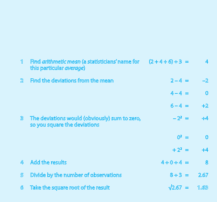
Calculating standard deviation
If you ever need to calculate standard deviation, you will use a calculator or a
computer spreadsheet. However, if you really want to know how it is done, this is
the procedure. To calculate the average (4) and standard deviation (1.63) of the
three numbers: 2, 4 and 6:
1 Find arithmetic mean (a statisticians’ name for
this particular average)
(2 + 4 + 6) ÷ 3 = 4
2 Find the deviations from the mean 2 – 4 = –2
4 – 4 = 0
6 – 4 = +2
3 The deviations would (obviously) sum to zero,
so you square the deviations
– 2
2
= +4
0
2
= 0
+ 2
2
= +4
4 Add the results 4 + 0 + 4 = 8
5 Divide by the number of observations 8 ÷ 3 = 2.67
6 Take the square root of the result √2.67 = 1.63
260 CHAPTER 11 MANAGING RISKS
You can pick any number in column A. For example, take 0.5. The corresponding value
in column B is about 30%. So, 30% of trees exceed the average by half a metre or more.
There is a 30% likelihood that sales will exceed $10.5 million.
The distribution of values is symmetrical. So for the previous example, you can also say
that 70% of trees are shorter than 10.5 metres. You can turn it upside down also. Thirty per
cent are shorter than 9.5 metres; 70% are taller than 9.5 metres. Just in case you are not
too fond of subtracting from 100, column C does it for you. Put another way, column B +
column C = 100%.
Columns B and C look at one side of the picture. They reveal how much of a normal
distribution lies on either side of a specific point. Columns D and E relate to both sides of
the middle. Go back to the $1 million example. Against 1 in column A, column E indicates
that there is a 68% probability that sales will be within (i.e. plus or minus) $1 million of
expected value – between $9 million and $11 million. Column D says that there is a 32%
chance that they won’t be. Clearly, columns D and E must also add to 100%.
IN THE REAL WORLD
I do not know about you, but I am seriously weary of all these numbers. Hang in there a
little longer, there is only one more step and it is the most interesting one. This is how you
apply all this to real-world situations.
1 Make a realistic (be honest) central observation, estimate or forecast.
2 Make a realistic second observation, estimate or forecast.
3 Attach a probability to the value in step 2.
4 Find the standard deviation implied by step 3.
5 Use this to estimate other values.
Box A opposite takes you step by step through the process of finding standard deviation.
For example, if you estimate that a machine can produce 150 widgets, but there is a 10%
chance that it will stamp out only 126, you can establish that the standard deviation for
this situation is 20.
Armed with the standard deviation you can do one of the following.
1 Choose any other value, find the z score and read off the percentage likelihood of
that value (see Box B on page 262). For example, if you chose 126 you would find
that there is a 10% chance of making this many or fewer widgets.
2 Choose any percentage, read off the z score, and convert it into a useful value. (See
Box C on page 262.) For example, there is a 90% likelihood of producing 176 or
fewer widgets.
..................Content has been hidden....................
You can't read the all page of ebook, please click here login for view all page.