Introduction

Market timing doesn’t work! At least that’s what some people would like you to think. The Random Walk Theory and the efficient market hypothesis tell investors market timing is a fool’s game. Academics have made careers out of ridiculing market timing. Mutual fund companies have issued hundreds, if not thousands, of reports deriding market timing while extolling “buy and hold,” pointing out the investment disaster that awaits any investor who happens to miss the biggest up days in a bull market. (Curiously absent are similar reports about investment performance when missing the biggest down days.) Without a doubt, successful market timing is not easy. But it’s not impossible, and when properly applied, market timing can generate big rewards for the time and effort expended.

We should emphasize that the equity market timing discussed in this book is not short-term in nature. No attempt is made to formulate short-term or day-trading timing strategies. The timing methods described in the following pages are aimed at the longer-term investor whose main interest is participating in the market’s primary uptrends—bull markets—while avoiding the primary downtrends—bear markets. Thus, traders looking for systems detailing short-term entry and exit points for the market or for money-management techniques should seek advice elsewhere. Our intent is to provide investors with techniques for identifying major market tops and bottoms in the equity market based on the works of two masters of market analysis, Lyman M. Lowry and Richard D. Wyckoff.

Not all market cycles, though, are created equal in terms of benefiting from market timing. In a secular bull market, timing is of secondary importance to a buy and hold strategy, as the cyclical bear markets within the longer-term uptrend tend to be relatively shallow and short-lived. Make no mistake, successful timing will improve investment performance even within a secular bull trend. But timing becomes paramount during periods of secular bear markets. For instance, as of this writing, the S&P 500 Index is at the same level as in November 2004. In other words, an investment in a fund that tracks the S&P 500 would have resulted in no net gains, ex-dividends, over the past six years.

At this point, we should probably define what we mean by a secular bull market versus a secular bear market. First of all, what do we mean by “secular?” We don’t mean temporal versus religious—although it could be argued some approach market analysis with religious fervor. We have to look all the way down to the third choice in the dictionary to find the applicable definition: “of or relating to a long term duration.” Thus, we have the shorter term cyclical bull markets within a secular bear or a cyclical bear within a secular bull.

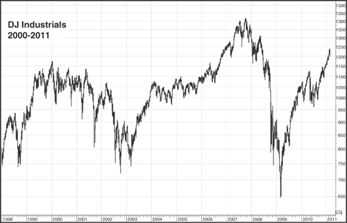
Now we have the definitions, but what are the characteristics that differentiate a secular market from a cyclical market? The key element differentiating a secular bull from secular bear is in the performance of the major price indexes themselves. In a secular bull market, bear markets tend to be short-lived, hence their characterization as “cyclical” bear markets. The lows in these bear markets also are far above previous bear market lows in the secular uptrend. For instance, the low in the 1984 bear market was well above the 1982 low, while the 1987 low was well above the ’84 low, and so on. This is not true in a secular bear market. In the 1966–82 secular bear market, the 1970 low was well below the 1966 low, while the 1975 bottom was far below the 1970 low. See Figure I.1 for an illustration of these secular bull and secular bear patterns. In addition, the relative level of cyclical bear market lows appears to offer an early warning a secular bull is about to end. Although the 1942–1966 secular bull market did not top until 1966, the low in the 1962 bear market fell below the low of the 1960 bear—breaking a string of higher lows dating to 1946. Similarly, the March 2003 bear market low was below the low in the 1998 bear market (Figure I.2), breaking the string of higher lows in ’84, ’87, ’90 and ’98. This March ’03 lower low plus the strong relative performances of new leaders in the energy, basic materials, and consumer cyclical stocks provided clear evidence the secular bull dating to the 1982 low had come to an end and signaled the start of a secular bear that, as of this writing, is still with us.

Figure I.1. DJIA Secular Bear Market 1966-1982 and Secular Bull Market 1982-2000

Charts created with Metastock, a Thomson Reuters product.

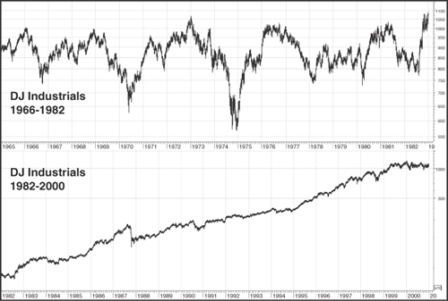
Figure I.2. Secular Bear Market 2000-2011 (thus far)

Charts created with Metastock, a Thomson Reuters product.

The emergence of new market leadership can be a key indication a shift from a secular bear to a secular bull (or vice versa) is taking place. For instance, the end of the 1966–1982 secular bear market was marked by a shift from stocks benefiting from inflation, such as metals (including gold), energy, and other commodity-based stocks, to those that would benefit from disinflation, such as consumer staples and finance stocks. The shift from the 1982–2000 secular bull market to a secular bear was marked by a similar shift away from technology and telecom stocks toward the basic materials, energy and consumer cyclical stocks that would lead in the 2003–2007 cyclical bull market. In both the 1982 and 2000 instances, the new leaders clearly outperformed the broad market indexes during the bear market, providing an early warning of a secular change in trend.

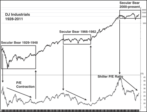
In addition to price, a second key element for identifying a secular bear market is the price/earnings ratio (or commonly referred to as the P/E ratio) for a major market index such as the S&P 500. The P/E ratio is based on the current price of the Index and, most frequently, the trailing 52-week combined earnings of the companies in the S&P 500. A secular bear market is characterized by a sustained contraction in the P/E Ratio, while in a secular bull market, the P/E Ratio shows a pattern of sustained expansion. Figure I.3 illustrates this pattern of contraction and expansion, using the inflation-adjusted average P/E Ratio for the S&P 500 on a rolling 10-year basis originated by Robert Shiller. As is evident, the P/E Ratio contracts steadily during the secular bear markets 1929-1948 and 1966-1982. In contrast, the Ratio expands during the secular bull markets 1948-1966 and 1982-2000. Based on these historic patterns, the sharp drop in the P/E Ratio since 2000 suggests the stock market is again in a secular bear trend.

Figure I.3. S&P 500 Price/Earnings Ratio in Secular Bear Markets

Charts created with Metastock, a Thomson Reuters product.

To sum up, a secular bull market is characterized by steady, long-term uptrends in the major price indexes, interrupted from time to time by shallow and short-lived cyclical bear markets. A secular bear market is characterized by a series of bull and bear markets in which the major price indexes make little or no upside progress. This lack of progress was well-illustrated by the 1966–1982 bear market where the DJIA made an initial high just above 1000 in 1966 and then failed to exceed that high by an appreciable amount until November 1982. As noted earlier, a similar lack of progress is evident in today’s market.

What does all this talk about secular bull and bear markets mean to an investor? In monetary terms, it means a lot. Despite all the ink spilled over the effects of missing x number of the biggest up days in a bull market, missing a bear market can be even more important for long-term investors. For example, in the 2007–2009 bear market, the S&P 500 suffered a drop of about 57%. This sickening drop was followed by an exhilarating rally of 80% in 2009–2010. Exhilarating, that is, for someone who had not just gone through the prior bear market. A hypothetical index fund investment of $100,000 at the market peak in 2007 would have dropped in value to just $43,000 by the time the S&P 500 bottomed out in March 2009. (For simplicity’s sake, we’re not factoring in dividends.) But what goes down comes back a lot slower because an 80% gain on $43,000 results in just $77,400, leaving our hypothetical investor still nearly $23,000 below his original $100,000. Ouch.

But, that’s just one bear market. The longer-term impact of a secular bear market, which entails a number of cyclical bull and bear markets, can be even more dramatic. For example, the current secular bear market is presumed to have begun at the March 2000 market peak with the S&P 500 at 1527.35. Yet at the time of this writing, the S&P was at 1181, or nearly 23% below its 2000 peak. Thus, despite the 101% gain for the S&P 500 in the 2003–2007 bull market, and the Index’s 80% gain in 2009–2010, our index fund investment would still be far below its value more than ten years before.

The secular bear market in place from 1966 to 1982, during which the DJIA (and S&P 500) failed to move appreciably above their 1966 highs tells a similar tale. In this case, we use the DJIA for our calculations, given that it was, at the time, the most widely followed index. From its 1966 high to its peak in 1981, the DJIA gained 2.9% (again, ignoring dividends). Thus, a $100,000 dollar investment would have appreciated to $102,900. Given the inflation of the late 1970s, it is likely an investor would have been less than impressed with this return, especially in terms of real (inflation-adjusted) dollars.

Historically, picking a bear market low or bull market high has been more associated with luck than with skill. But what if, through use of market timing, an investor was able to exit the market 10% below its bull market peak and then re-enter 20% above its bear market low? That’s a substantial haircut from getting out at the top and in at the bottom. In this case, our hypothetical index fund investment of $100,000 at the 1966 high would have appreciated to $143,900 by the market high in 1981—not bad, considering the delayed exit and entry points. Using the methods developed by L.M. Lowry and Richard D. Wyckoff, though, it has been possible to identify the peaks and troughs of bull and bear markets much more accurately. In fact, using the entry and exit points based on the principles detailed in the following pages, our hypothetical 1966 $100,000 investment would have grown to $204,400 by the time the market peaked in 1981.

Let’s be more specific here about the goals of this book. Richard D. Wyckoff (who you learn more about in the first chapter) identified specific market actions in terms of price and volume relationships, which he utilized, successfully, to identify turning points in equity price trends. A little later on, L.M. Lowry developed measures that quantify and display changes in the trends of Supply and Demand that are behind changes in equity price trends. Our aim is to enable an investor to recognize those actions that identify major changes in trend and to differentiate them from the day to day movements in the stock market. We do this by reviewing the major market tops and bottoms in the 1966–82 and 2000–present secular bear markets, identifying and explaining the key characteristics of each market action as it applies to the formation and conclusion of the major market tops and bottoms. We then go on to identify and illustrate some other tools useful in recognizing major market tops and bottoms and continue with a case study of the 2000–2001 market top (which was in many ways unique) and conclude with a discussion of the current market.

The primary measures of the forces of Supply and Demand we use along with the Wyckoff analysis are the Buying Power and Selling Pressure Indexes, which form the basis of the Lowry analysis. Many indicators have been developed to measure changes in Supply and Demand, from On Balance Volume to various money flow and accumulation/distribution indicators. However, Buying Power and Selling Pressure are the only indicators of which we are aware to measure changes in Supply and Demand independently, rather than plotting changes as a single line. This allows for the application of the two Indexes in analyzing the major trends of the stock market well beyond their use in this book for identifying major tops and bottoms. We realize Buying Power and Selling Pressure are propriety indicators to Lowry Research and, as such, available only to subscribers. Nonetheless, we have found these indicators best complement the Wyckoff analysis in measuring the forces of Supply and Demand at major market tops and bottoms. Readers should note that the application of the Lowry indicators to the Wyckoff method is meant to illustrate how the analyses of these two masters work together. It is certainly possible to conduct an examination of major market tops and bottoms on the basis of the Wyckoff analysis alone (which is demonstrated in Chapter 9 through an analysis of the NASDAQ Composite Index top in 2000). Readers interested in a more complete coverage of the Wyckoff analysis can contact the Wyckoff Stock Market Institute in Phoenix, Arizona, which has available a study course based on Mr. Wyckoff’s original correspondence course introduced in the early 1930s.