
The most frustrating part of a complex modeling job is to be able to envision a result, but not be able to create it because you do not have the tools to get it done. Worse yet is to actually have the tools but either not understand how to use them or not even realize that you have them. Getting the job done is so much more satisfying when you use the right tools and get the job done right — not just so that it looks right, but so that it really is right.
SolidWorks offers so many tools that it is sometimes difficult to select the best one, especially if it is for a function that you do not use frequently.
This chapter helps you identify which features to use in which situations, and in some cases, which features to avoid. It also helps you evaluate which feature is best to use for a particular job. With some features, it is clear when to use them, but for others, it is not. This chapter guides you through the decision-making process.
I am always trying to think of alternate ways of doing things. It is important to have a backup plan, or sometimes multiple backup plans, in case a feature doesn't perform exactly the way you want it to. As you progress into more complex features, you may find that the more complex features are not as well behaved as the simple features. You may be able to get away with only doing blind extrudes and cuts with simple chamfers and fillets for the rest of your career. In addition, even if you could, would you want to?
As an exercise, I often try to see how many different ways a particular shape might be modeled, and how each modeling method relates to manufacturing methods, costs, editability, efficiency, and so on. You may also want to try this approach for fun or for education.
As SolidWorks grows more and more complex, and the feature count increases with every release, understanding how the features work and how to select the best tool for the job becomes ever more important. If you are only familiar with the standard half-dozen or so features that most users use, your options are limited. Sometimes simple features truly are the correct ones to use, but using them because they are the only things you know is not always the best choice.
The "Base" part of the Extruded Boss/Base is a holdover from when SolidWorks did not allow multi-body parts, and the first feature in a part had special significance that it no longer has. This is also seen in the menus at Insert
Cross-Reference
Multi-body parts are covered in detail in Chapter 26.
In this case, the term solid feature is used as an opposite of thin feature. This is the simple type of feature that you create by default when you extrude a closed loop sketch. A closed loop sketch fully encloses an area without gaps or overlaps at the sketch entity endpoints. Figure 7.1 shows a closed loop sketch creating an extruded solid feature. This is the default type of geometry for closed loop sketches.
The Thin Feature option is available in several features, but is most commonly used with Extruded Boss features. Thin features are created by default when you use open loop sketches, but you can also select the Thin Feature option for closed loop sketches. Thin features are commonly used for ribs, thin walls, hollow bosses, and many other types of features that are common to plastic parts, castings, or sheet metal.
Even experienced users tend to forget that thin features are not just for bosses, but that they can also be used for cuts. For example, you can easily create grooves and slots with thin feature cuts.
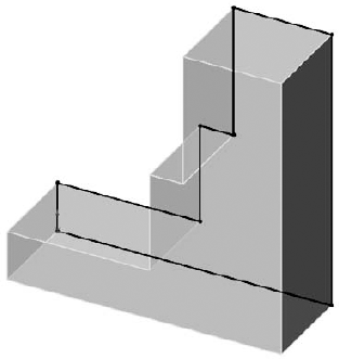
Figure 7.2 shows the Thin Feature panel in the Extruded Boss PropertyManager. In addition to the default options that are available for the extrude feature, the Thin feature adds a thickness dimension, as well as three options to direct the thickness relative to the sketch: One-Direction, Mid-Plane, and Two-Direction. The Two-Direction option requires two dimensions, as shown in Figure 7.2.

Thin feature sketches are typically simpler than closed loop sketches, which usually means that they are more robust through changes. You can create the simplest cube from a single sketch line and a thin feature extrude. However, because they are more specialized in some respects, they are not as flexible when the design intent changes. For example, if a part is going to change from a constant width to a tapered or stepped shape, thin features do not handle this kind of change. Figure 7.3 shows different types of geometry that are typically created from thin features.
I have already mentioned several sketch types, including closed loop and open loop. Closed loop sketches make solid features by default, but you can also use them to make thin features. Open loop sketches make thin features by default, and you cannot use them to make solid features. A nested loop is one closed loop inside another, like concentric circles. Self-intersecting sketches can be any type of sketch where the geometry crosses itself. SolidWorks also identifies sketches where three or more sketch elements intersect at a point by issuing an error if you try to use the sketch in a feature.
SolidWorks works best with well-disciplined sketches that follow the rules. Therefore, if you plan to use sketch contours, you should make sure that it is not simply because you are unwilling to clean up a messy sketch.
When you define features by selecting sketch contours, they are more likely to fail if the selection changes when the selected contour's bounded area changes in some way. It is considered best practice to use the normal closed loop sketch when you are defining features. Contour selection is best suited to "fast and dirty" conceptual models, which are used in very limited situations.
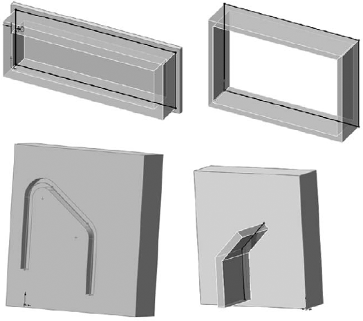
There are several types of contour selection, as shown in Figure 7.4.
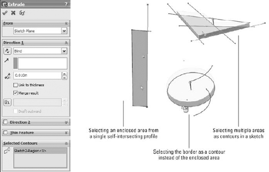
The terminology used by SolidWorks is not always logical, for example, the heading of the PropertyManager panel that you use is called Selected Contours, but the item in the selection box is called a Region. This is why you may sometimes hear Contours referred to as Regions.
You can make extrusions from 3D sketches, even 3D sketches that are not planar. While not necessarily the best way to do extrudes, this is a method that you can use when needed. You can establish direction for an extrusion by selecting a plane (normal direction), axis, sketch line, or model edge.
When you make an extrusion from a 3D sketch, the direction of extrusion cannot be assumed or inferred from anything — it must be explicitly identified. Extrusion direction from a 2D sketch is always perpendicular to the sketch plane unless otherwise specified.
Non-planar sketches become somewhat problematic when you are creating the final extruded feature. The biggest problem is how you cap the ends. Figure 7.5 shows a non-planar 3D sketch that is being extruded. Notice that the end faces are, by necessity, not planar, and are capped by an unpredictable method, probably a simple Fill surface. This is a problem only if your part is going to use these faces in the end; if it does not, then there may be no issue with using this technique. If you would like to examine this part, it is included on the CD-ROM as Chapter 7 Extrude 3D Sketch.sldprt.

If you need to have ends with a specific shape, and you still want to extrude from a non-planar 3D sketch, then you should use an extruded surface feature rather than an extruded solid feature.
One big advantage of using a 3D sketch to extrude from is that you can include profiles on many different levels, although they must all have the same end condition. Therefore, if you have several pockets in a plate, you can draw the profile for each pocket at the bottom of the pocket, and extrude all the profiles Through All, and they will all be cut to different depths.
3D sketches also have an advantage when all the profiles of a single loft or boundary are made in a single 3D sketch. This enables you to drag the profiles and watch the loft update in real time.
Cross-Reference
Surfacing features are covered in detail in Chapter 27. Chapter 4 contains additional details on extrude end conditions, thin features, directions, and the From options. Chapter 31 also has more information on 3D sketches.
Instant 3D enables you to select a sketch or a sketch contour and drag the Instant 3D arrow to create either a blind extruded boss or cut. The workflow when using this function requires that the sketch be closed. Instant 3D cannot be used to create a thin feature, and any sketch or contour that it uses must be a closed loop. Sketches must also be shown (not hidden) in order to be used with Instant 3D.
Note
Even though the words "Instant 3D" suggest that you should be able to instantly create 3D geometry from a sketch that you may have just created, you do have to close the sketch first to get instant functionality. In this case, Instant 3D requires the sketch to be closed (as in not active) and closed (as in not an open loop.
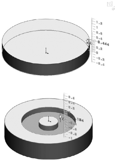
Figure 7.6 shows Instant 3D arrows for extruding a sketch into a solid and the ruler to establish blind extrusion depth. These extrusions were done from a single sketch with three concentric circles, using contour selection.
Even after you create an extruded boss, you can use Instant 3D to drag it in the other direction to change the boss into an extruded cut. When you do this, the symbol on the feature changes, but the name does not.
If you have a sketch that requires contour selection, SolidWorks automatically hides the sketch, and to continue with Instant 3D functionality using additional contours selected from that sketch, you will have to show the sketch again. This interrupts the workflow and makes using this functionality less fluid than it might otherwise be. I only mention it here so that you are aware of what is happening when the sketch disappears and the Instant 3D functionality disappears with it.
If geometry already exists in the part, and you drag a new feature into the existing solid, SolidWorks assumes you want to make a cut. However, maybe you are really trying to make a boss that comes out the other side of the part. These heads-up display icons enable you to do this. Options include boss, cut, and draft. The draft option enables you to add draft to a feature created with Instant 3D.
While Instant 3D can only create extruded bosses and cuts, it can edit revolves. If you create a revolved feature revolving the sketch, say, 270°, the face created at the angle can be edited by Instant 3D dragging. You can also drag faces created by any underdefined sketch elements.
Instant 3D enables you to edit 2D sketches and solid geometry. You can also edit some additional feature types using Instant 3D, such as offset reference planes. It can neither create nor edit surface geometry or 3D sketches in some situations. To edit solid geometry, click on a face, and an arrow appears. Drag the arrow, and SolidWorks automatically changes either the sketch or the feature end condition used to create that face. If a dimensioned sketch was used to create that face, SolidWorks will not allow you to use the Instant 3D arrow to move or resize the face. An option exists that enables Instant 3D changes to override sketch dimensions at Tools
Warning
Be careful with the Override Dims on Drag option. If you accidentally drag a fully defined sketch, this setting enables SolidWorks to completely resize the sketch. For working conceptually, it can be a great aid, but for final production models, you may do better to turn this off.
Instant 3D offers different editing options depending on how a sketch is selected.
A sketch is selected from the graphics window. The pull arrow appears, enabling you to create an extruded boss or cut.
A sketch is selected from the FeatureManager. If the sketch has relations to anything outside of the sketch, the sketch is highlighted with no special functionality available. If no external relations exist, a box with stretch handles enable scaling the sketch, and a set of axes with a wing enables you to move the sketch in X or Y or X and Y. Figure 7.7 shows this situation.
When Instant 3D is activated, double-clicking a sketch in either the FeatureManager or on a sketch element in the graphics window opens that sketch. While you are in a sketch, if you double-click with the Select cursor in blank space in the graphics window, you close the sketch. This only works for 2D sketches; 3D sketches can be opened, but not closed, this way.

Draw only half of the revolve profile. (Draw the section to one side of the centerline.)
The profile must not cross the centerline.
The profile must not touch the centerline at a single point. It can touch along a line, but not at a point. Revolving a sketch that touched the centerline at a single point would create a point of zero thickness in the part.
You can use any type of line or model edge for the centerline, not just the centerline/construction line type.
There are three Revolve end conditions:
There is no equivalent for Up to Vertex, Up to Next, Up to Surface, or Up to Body with the Revolve feature.
Many users struggle when faced with the option to create a loft or a sweep. Some overlap exists between the two features, but as you gain some experience, it becomes easier to choose between them. Generally, if you can create the cross-section of the feature by manipulating the dimensions of a single sketch, a sweep might be the best feature. If the cross-section changes character or severely changes shape, a loft may be best. If you need a very definite shape at both ends and/or in the middle, a loft is a better choice because it enables you to explicitly define the cross-section at any point. However, if the outline is more important than the cross-section, you should choose a sweep. In addition, if the path between ends is important, choose a sweep.
Both types of features are extremely powerful, but the sweep has a tendency to be fussier about details, setup, and rules, while the loft can be surprisingly flexible. I am not trying to dissuade you from using sweeps, because they are useful in many situations. However, in my own personal modeling, I probably use about ten lofts for every sweep. For example, while you would use a loft or combination of loft features to create the outer faces of a complex laundry detergent bottle, you would use the sweep to create a raised border around the label area or the cap thread.
A good example of the interpolated nature of a loft is to put a circle on one plane and a rectangle on an offset plane and then loft them together. This arrangement is shown in Figure 7.8. The transition between shapes is the defining characteristic of a loft, and is the reason for choosing a loft instead of another feature type. Lofts can create both Boss features and Cut features.
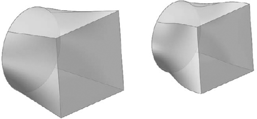
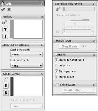
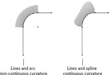
Both shapes are two-profile lofts. The two-profile loft with default end conditions always creates a straight transition, which is shown in the image to the left. A two-point spline with no end tangency creates a straight line in exactly the same way. By applying end conditions to either or both of the loft profiles, the loft's shape is made more interesting, as seen in the image to the right in Figure 7.8. Again, the same thing happens when applying end tangency conditions to a two-point spline: it goes from being a straight line to being more curvaceous, with continuously variable curvature. The Loft PropertyManager interface is shown in Figure 7.9.
For solid lofts, you can select faces, closed loop 2D or 3D sketches, and surface bodies. You can use sketch points as a profile on the end of a loft that comes to a point or rounded end. For surface lofts, you can use open sketches and edges in addition to the entities that are used by solid lofts.
Some special functionality becomes available to you if you put all the profiles and guide curves together in a single 3D sketch. In order to select profiles made in this way, you must use the SelectionManager, which is discussed later in this chapter.
The Sketch Tools panel of the Loft PropertyManager enables you to drag sketch entities of any profile made in this way while you are editing or creating the Loft feature, without needing to exit and edit a sketch.
Note
I discuss 3D sketches in more detail in Chapter 31.
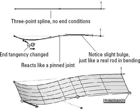
The words loft and spline come from the shipbuilding trade. The word spline is actually defined as the slats of wood that cover the ship, and the spars of the hull very much resemble loft sections. With the splines or slats bending at each spar, it is easy to see how the modern CAD analogy came to be.
Lofts and splines are also governed by similar mathematics. You have seen how the two-point spline and two-profile loft both create a straight-line transition. Next, a third profile is added to the loft and a third point to the spline, which demonstrates how the math that governs splines and lofts is also related to bending in elastic materials. Figure 7.10 shows how lofts and splines react geometrically in the same way that bending a flexible steel rod would react (except that the spline and the loft do not have a fixed length).
With this bit of background, it is time to move forward and talk about a few of the major aspects of loft features in SolidWorks. It is possible to write a separate book that only discusses modeling lofts and other complex shapes. This has in fact been done. The SolidWorks Surfacing and Complex Shape Modeling Bible (Wiley, 2008) covers a wide range of surfacing topics with examples in far detail. In this single chapter, I do not have the space to cover the topic exhaustively, but coverage of the major concepts will be enough to point you in the right direction.
In this chapter, I deal exclusively with solid modeling techniques because they are the baseline that SolidWorks users use most frequently. Surfaces make it easier to discuss complex shape concepts because surfaces are generally created one face at a time, rather than by using the solid modeling method that creates as many faces as necessary to enclose a volume.
From the very beginning, the SolidWorks modeling culture has made things easier for users by taking care of many of the details in the background. This is because solids are built through automated surface techniques. Surface modeling in itself can be tedious work because of all the manual detail that you must add. Solid modeling as we know it is simply an evolutionary step that adds automation to surface modeling. The automation maintains a closed boundary of surfaces around the solid volume.
Because surfaces are the underlying building blocks from which solids are made, it would make sense to teach surfaces first, and then solids. However, the majority of SolidWorks users never use surfacing, and do not see a need for it; therefore, surface functions are generally given a lower priority.
Cross-Reference
Refer to Chapter 27 for surfacing information. For a comprehensive look at surfacing and complex shapes, see the SolidWorks Surfacing and Complex Shape Modeling Bible (Wiley, 2008).
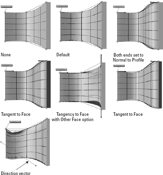
Loft end conditions control the tangency direction and weighting at the ends of the loft. Some of the end constraints depend upon the loft starting or ending from other geometry. The optional constraints are covered in the following sections.
The direction of the loft is not set by the None end constraint, but the curvature of the lofted faces at the ends is zero. This is the default end constraint for two-section lofts.
The Default end constraint is not available for two-section lofts, only for lofts with three or more sections. This end constraint applies curvature to the end of the loft so that it approximates a parabola being formed through the first and last loft profiles.
The Tangent to Face end constraint is self-explanatory. The Tangency to Face option includes a setting for tangent length. This is not a literal length dimension, but a relative weighting, on a scale from 0.1 to 10. The small arrow to the left of the setting identifies the direction of the tangency. Usually, the default setting is correct, but there are times when SolidWorks misidentifies the intended tangency direction, and you may need to correct it manually.
The Next Face option is available only when lofting from an end face where the tangency could go in one of two perpendicular directions. This is shown in Figure 7.11.
Apply to All refers to applying the Tangent Length value to all the tangency-weighting arrows for the selected profile. When you select Apply to All, only one arrow displays. When you deselect it, one arrow should display for each vertex in the profile, and you can adjust each arrow individually.
The difference between tangency and curvature is that tangency is only concerned with the direction of curvature immediately at the edge between the two surfaces. Curvature must be tangent and match the radius of curvature on either side of the edge between surfaces. This is often given many names, including curvature continuity and c2 or g2. Lofted surfaces do not usually have a constant radius; because they are like splines, they are constantly changing in local radius.
The Direction Vector end constraint forces the loft to be tangent to a direction that you define by selecting an axis, edge, or sketch entity. The angle setting makes the loft deviate from the direction vector, as shown in Figure 7.11. The curved arrows to the left identify the direction in which the angle deviation is going.
The mesh or grid shown in the previous images appears automatically for certain types of features, including lofts. The grid represents isoparameter lines, also known as NURBS mesh or U-V lines. This mesh shows the underlying structure of the faces being created by the feature. If the mesh is highly distorted and appears to overlap in places, then it is likely that the feature will fail.
You can show or hide the mesh through the right mouse button (RMB) menu when editing or creating a Loft feature, unless the SelectionManager is active. In this case, you can see only SelectionManager commands in the RMB menu. In addition, planar faces do not mesh, only faces with some curvature.
Guide curves help to constrain the outline of a loft between loft profiles. Although it is best to try to achieve the shape you want by using appropriately shaped and placed loft profiles, this is not always possible. The most appropriate use of guide curves for solid lofts is at places where the loft is going to create a hard edge, which is usually at the corners of loft profile sketches. Guide curves often (but not always) break up what would otherwise be a smooth surface, and you should avoid them in these situations, if possible.
Best Practice
Do not try to push the shape of the loft too extremely with guide curves. Use guide curves mainly for tweaking and fine-tuning rather than coarse adjustments. Use loft sections and end constraints to get most of the overall shape correct. Pushing too hard with a guide curve can cause the shape to kink unnaturally.
Although guide curves can be longer than the loft, they can not be shorter. The guide curve applies to the entire loft. If you need to apply the guide curve only to a portion of the loft, then split the loft into two lofts: one that uses the guide curve and one that does not. The guide curve must intersect all profiles in a loft.
If you have more than one guide curve, the order in which they are listed in the box is important. The first guide curve helps to position the intermediate profiles of the loft. It may be difficult to visualize the effects of guide-curve order before it happens, but remember that it does make a difference, and depending on the difference between the curves, the difference may or may not be subtle.
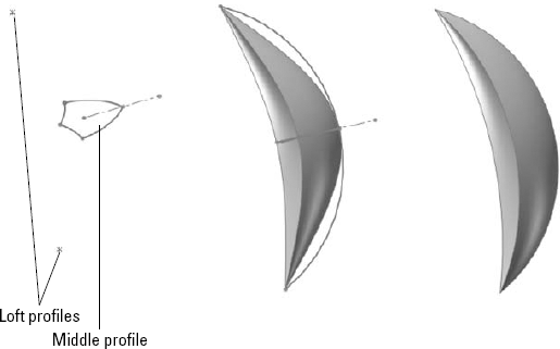
Guide curves are also used in sweeps, which I address later in this chapter. Figure 7.12 shows a model that is lofted using guide curves. The image to the left shows the sketches that are used to make the part. There are two sketches with points; you can use points as loft profiles. The image in the middle shows the Loft feature without guide curves, and the one to the right is the part with guide curves. If you would like to examine how this part is built, you can find it on the CD-ROM with the filename Chapter 7 Guide Curves.sldprt.
The Centerline panel of the Loft PropertyManager is used to set up a centerline loft. You can use the centerline of a loft in roughly the same way that you use a sweep path. In fact, the Centerline loft resembles a sweep feature where you can specify the shape of some of the intermediate profiles. Centerline lofts can also create intermediate profiles. You may prefer to use a centerline loft instead of either a sweep or a regular loft because the profile may change in ways that the Sweep feature cannot handle, and the loft may need some guidance regarding the order of the profiles, or how to smooth the shape between the profiles.
I cover sweep features in this chapter. If you are creating a centerline loft, you may want to examine the sweep functionality as well.
You can use centerlines simultaneously with guide curves. While guide curves must touch the profile, there is no such requirement for a centerline; in fact, the centerline works best if it does not touch any of the profiles.
The slider in the Centerline Parameters panel enables you to specify how many intermediate sections to create between sketched profiles.
The SelectionManager simplifies the selection of entities from complex sketches that are not necessarily the clean, closed loop sketches that SolidWorks works with most effectively.
The SelectionManager has been implemented in a limited number of features. Selection options in the SelectionManager include the following:


A parametric closed loop in a 2D or 3D sketch.
A parametric loop of edges around a surface.


Auto OK Selections. Becomes enabled when you use the Push Pin. Auto OK Selections works for closed and open loop selection.
You can choose from the following Loft options, as shown in Figure 7.13:
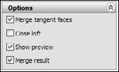
Merge tangent faces. Merges model faces that are tangent into a single face. This is done behind the scenes by converting profiles into splines, which make approximations but are smoother than sketches with individual tangent line and arc entities.
Close loft. The loft is made into a closed loop. At least three loft profiles must exist in order to use this option. Figure 7.14 shows a loft where the Close Loft option is used, and the loft sections are shown. This model is on the CD-ROM with the filename Chapter 7 —
Closed Loft.sldprt.Show preview. Selecting and deselecting this option turns the preview of the Loft feature on or off, respectively, if the feature is going to work. All the following loft preview options are system options and remain selected until you deselect them.
Transparent/Opaque Preview is available from the RMB menu when you edit a loft, if the SelectionManager is not active.
Mesh Preview is also available on the same RMB menu.
Zebra Stripe Preview is also available on the same RMB menu, and is covered in more depth in Chapter 11.
Merge result. Merges the resulting solid body with any other solid bodies that it may contact.

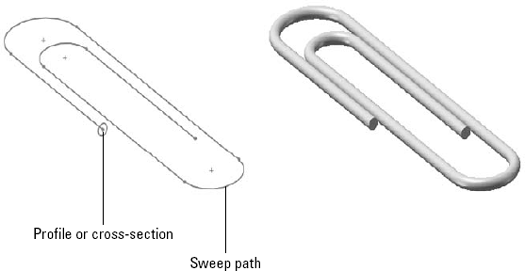
The main criteria for selecting a sweep to create a feature are that you must be able to identify a cross-section and a path. The profile (cross-section) can change along the path, but the overall shape must remain the same. The profile is typically perpendicular to the path, although this is not a requirement.
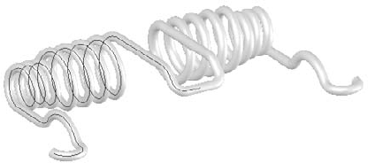
An example of a simple sweep is shown in Figure 7.15. The paper clip uses a circle as the profile and the coiled lines and arcs as the path.
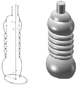
Sweeps that are more complex begin to control the size, orientation, and position of the cross-section as it travels through the sweep. When you use a guide curve, several analogies can be used to visualize how the sweep works. The cross-section/profile is solved at several intermediate positions along the path. If the guide curve does not follow the path, the difference between the two is made up by adjusting the profile. Consider the following example. In this case, the profile is an ellipse, the path is a straight line, and there are guide curves that give the feature its outer shape. Figure 7.16 shows all these elements and the finished feature.
On the CD-ROM
The part shown in Figure 7.16 is on the CD-ROM with the filename Chapter7 Bottle.sldprt.
The PropertyManager for the Sweep function includes an option for Show Sections, which in this case creates almost 200 intermediate cross-sections. These sections are used behind the scenes to create a loft. You can think of complex sweeps with guide curves or centerlines as an automated setup for an even more complex loft. It is helpful to envision features such as this when you are troubleshooting or setting up sweeps that are more complex. If you open the part mentioned previously from the CD-ROM, you can edit the Sweep feature to examine the sections for yourself.
In most other published SolidWorks materials that cover these topics, sweeps are covered before lofts because many people consider lofts the more advanced topic. However, I have put lofts first because understanding them is necessary before you can understand complex sweeps, as complex sweeps really are just lofts.
The Pierce sketch relation is the only sketch relation that applies to a 3D out-of-plane edge or curve without projecting the edge or curve into the sketch plane. It acts as if the 3D curve is a length of thread and the sketch point is the eye of a needle where the thread pierces the needle eye. The Pierce relation is most important in the Sweep feature when it is applied in the profile sketch between endpoints, centerpoints, or sketch points and the out-of-plane guide curves. This is because the Pierce relation determines how the profile sketch will be solved when it is moved down the sweep path to create intermediate profiles.
Figure 7.17 illustrates the function of the Pierce relation in a sweep with guide curves. The dark section on the left is the sweep section that is sketched. The lighter sketches to the right represent the intermediate profiles that are automatically created behind the scenes, and are used internally to create the loft.
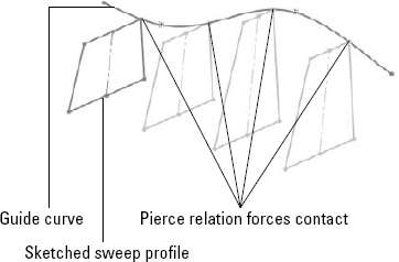
Figure 7.17 shows what is happening behind the scenes in a sweep feature. The sweep re-creates the original profile at various points along the path. The guide curve in this case forces the profile to rebuild with a different shape. Pierce constraints are not required in simple sweeps, but when you start using guide curves, you should also use a pierce.
Tip
If you feel that you need more profile control, but still want to create a sweep-like feature, try a centerline loft. The centerline acts like a sweep path that doesn't touch the profiles, but unlike a sweep, you can use multiple profiles with it.
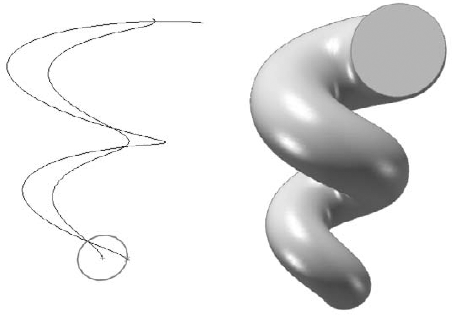
Figure 7.18 shows a more complicated 3D sweep, where both the path and the guide curve are 3D curves. I cover 3D curves toward the end of this chapter; you can refer to these sections to understand how this part is made.
On the CD-ROM
The part shown in Figure 7.18 is on the CD-ROM with the filename Chapter 7 3D Sweep.sldprt.
This part is created by making a pair of tapered helices, with the profile sketch plane perpendicular to the end of one of the curves. The taper on the outer helix is greater than on the inner one, which causes the twist to become larger in diameter as it goes up.
To make the circle follow both helices, you must create two pierce relations, one between the center of the circle and a helix, and the other between a sketch point that is placed on the circumference of the circle and the other helix. This means that the difference in taper angles between the two helices is what drives the change in diameter of the sweep.
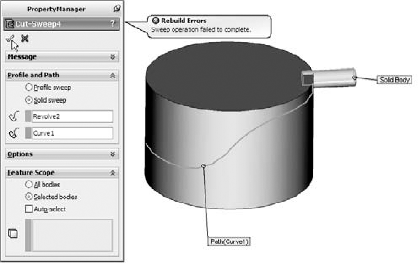
The Cut Sweep feature has an option to use a solid sweep profile. This kind of functionality has many uses, but is primarily intended for simulating complex cuts made by a mill or lathe. Figure 7.19 shows a couple of examples of cuts you can make with this feature. The part used for this screen shot is also on the CD-ROM.

The solid profile cut sweep has a few limitations that I need to mention:
It uses a separate solid body as the cutting tool, so you have to model multi-bodies.
The path must start at a point where it intersects the solid cutting tool body (path starts inside or on the surface of the cutting tool).
The cutting tool must be definable with a revolved feature.
The cutting tool must be made of simple analytical faces (sphere, torus, cylinder, and cone; no splines).
You cannot use a guide curve with a solid profile cut (cannot control alignment).
The cut can intersect itself, but the path cannot cross itself.
You can create many useful shapes with the solid profile cut sweep, but because of some of the limitations I've listed, some shapes are more difficult to create than others. For these shapes, you might choose to use regular cut sweep features. Figure 7.20 shows an example of a cam-like feature that you may want to create with this method, but may not be able to adequately control the cutting body.
Curves in SolidWorks are often used to help define sweeps and lofts, as well as other features. Curves differ from sketches in that curves are defined using sketches or a dialog box, and you cannot manipulate them directly or dimension them in the same way that you can sketches. Functions that you are accustomed to using with sketches often do not work on curves.
Several features that carry the curve name are actually sketch-based features:
Equation driven curve
Intersection curve
Face curves
Tip
When you come across a function that does not work using a curve entity, but that works on a sketch (for example, making a tangent spline), it may help to use the Convert Entities function. Converting a helix into a 3D sketch creates a spline that lies directly on top of the helix and enables you to make another spline that is tangent to the new spline.
You can define the following types of curves in SolidWorks:
Helix/tapered helix/variable helix/spiral
Projected curve
Curve through XYZ points
Curve through reference points
Composite curve
You can find all the curve functions on the Curves toolbar or by choosing Insert
Curve features in general have several limitations, some of which are serious. You have to be prepared with workaround techniques when using them. When curves are used in features, you often cannot reselect the curve to re-apply sketch broken sketch relations. (The work around for this is to select the curve from the FeatureManager, or if that doesn't work, you have to delete the feature and re-create it). In addition, curves cannot be mirrored, moved, patterned, or manipulated in any way. (A workaround for this may be to use Convert Entities to create a sketch from the curve.)
You can create all the helical curve types by specifying any combination of total height, pitch, and the number of revolutions. The start angle is best thought of as a relative number. It is difficult to predict where zero degrees starts, and this depends on the relation of the sketch plane to the Origin. The start angle cannot be controlled outside of the PropertyManager, and cannot be driven by sketch geometry. The term pitch refers to the straight-line distance along the axis between the rings of the helix. Pitch for the spiral is different and is described later.

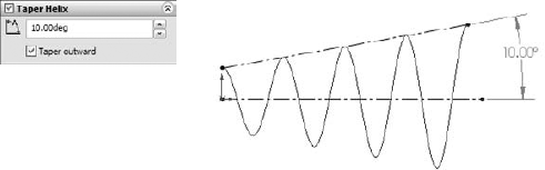
The Tapered Helix panel in the Helix PropertyManager enables you to specify a taper angle for the helix. The taper angle does not affect the pitch. If you need to affect both the taper and the pitch, then you can use a variable pitch helix. Figure 7.22 shows how the taper angle relates to the resulting geometry.
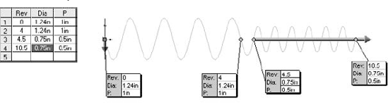
You can specify the variable pitch helix either in the chart or in the callouts that are shown in Figure 7.23. Both the pitch and the diameter are variable. The diameter number in the first row cannot be changed, but is driven by the sketch. In the chart shown, the transition between 4 and 4.5 revolutions is where the pitch and diameter both change.
Sketch On Faces
Sketch On Sketch
These names can be misleading if you do not already know what they mean. In both cases, the word sketch is used as a noun, not a verb, so you are not actively sketching on a surface; instead, you are creating a curve by projecting a sketch onto a face.
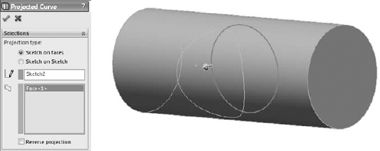
The Sketch On Faces option is the easiest to explain, so I will describe this one first. With this option set, the projected curve is created by projecting a 2D sketch onto a face. The sketch is projected normal (perpendicular) to the sketch plane. This is like extruding the sketch and using the Up To Surface end condition. The sketch can be an open or closed loop, but it may not be multiple open or closed loops, nor can it be self-intersecting. Figure 7.24 shows an example of projecting a sketch onto a face to create a projected curve.
This is the concept that most frequently causes difficulty for users. The Sketch Onto Sketch Projected Curve option can be visualized in a few different ways.
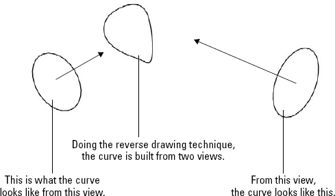
One way to visualize Sketch Onto Sketch projection is to think of it as being the reverse of a 2D drawing. In a 2D drawing, 3D edges (you can think of the edges as curves) are projected onto orthogonal planes to represent the edge from the Front or Top planes. The Sketch Onto Sketch projection takes the two orthogonal views, placed on perpendicular planes, and projects them back to make the 3D edge or curve. This is part of the attraction of the projected curve, because making 3D curves accurately is difficult if you do it directly by using a tool such as a 3D sketch spline; however, if you know what the curve looks like from two different directions, then it becomes easy. Figure 7.25 illustrates this visualization method.
When you think of describing a complex 3D curve in space, one of the first methods that usually comes to mind is describing it as two 2D curves from perpendicular directions, exactly in the same way as you would if you created projected drawing views from it. From this, it makes sense to see the creation of the curve as the reverse process, drawing the 2D views first, from which you can then create the 3D curve.
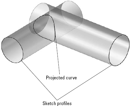
A second method used for visualizing Sketch On Sketch projected curves is the intersecting surfaces method. In this method, you can see the curve being created at the intersection of two surfaces that are created by extruding each of the sketches. This method is shown in Figure 7.26.
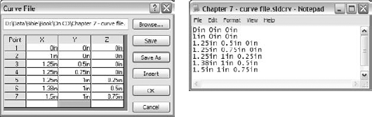
If you import a text file, the file can have an extension of either *.txt or *.sldcrv. The data that it contains must be formatted as three columns of X-, Y-, and Z-coordinates using the document units (inch, mm, and so on), and the coordinates must be separated by comma, space, or tab. Figure 7.27 shows both the Curve File dialog box displaying a table of the curve through X, Y, and Z points, and the *.sldcrv Notepad file. You can read the file from the Curve File dialog box by clicking the Browse button, but if you manually type the points, then you can also save the data out directly from the dialog box. Just like any type of sketch, this type of curve cannot intersect itself.
The most common application of this feature is to create a wire from selected points along a wire path. Another common application is a simple two-point curve to close the opening of a surface feature such as Fill, Boundary, or Loft.
Composite curves overlap in functionality with the Selection Manager to some extent. In some ways, the Composite Curve is nicer because you can save a selection in case the creation of the feature that uses the Selection Manager fails. (If you can't create the feature, you can't save the selection.) On the other hand, Composite Curves don't function the same way that a selection of model edges do for settings like tangency and curvature.
There are some limitations to using split lines. First, they must split a face into at least two fully enclosed areas. You cannot have a split line with an open loop sketch where the ends of the loop are on the face that is to be split; they must either hang off the face to be split or be coincident with the edges. If you think you need a split line from an open loop, try using a projected curve instead.
The SolidWorks 2010 version removes some other long-standing limitations, such as splitting on multiple bodies, using multiple closed loops, and using nested loops. These much needed improvements will help users avoid workarounds.
Warning
A word of caution is needed when using split lines, especially if you plan to add or remove split lines from an existing model. The split lines should go as far down the tree as possible. Split lines change the face IDs of the faces that they split, and often the edges as well. If you roll back and apply a split line before existing features, you may have a significant amount of cleanup to do. Similarly, if you remove a split line that already has several dependent features, many other features may also be deleted or simply lose their references.
SolidWorks offers very powerful filleting functions. The Fillet feature comprises various types of fillets and blends. Simple fillets on straight and round edges are handled differently from variable-radius fillets, which are handled differently from the single or double hold line fillet or setback fillets. Once you click the OK button to create a fillet as a certain type, you cannot switch it to another type. You can switch types only before you create an established fillet feature.
Many filleting options are available, but most of them are relatively little used or even known. In fact, most users confine themselves to the Constant Radius or Variable Radius fillets. The following section describes all the available fillet types and options:
Constant Radius Fillet
Multiple Radius Fillet
Round Corners
Keep Edge/Keep Surface
Keep Feature
Variable Radius Fillet
Face Fillet
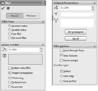
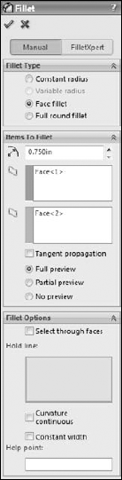
Figure 7.29 shows the Fillet PropertyManager. Other options affect preview and selection of items, and these options are discussed in this section.
Constant radius fillets are the most common type that are created if you select only edges, features, or faces without changing any settings. When applying fillets in large numbers, you should consider several best-practice guidelines and other recommendations that come later in this chapter.
There are still some long-time users who distinguish between fillets and rounds (where fillets add material and rounds remove it). SolidWorks does not distinguish between the two, and even two edges that are selected for use with the same fillet feature can have opposite functions; for example, both adding and removing material in a single feature.
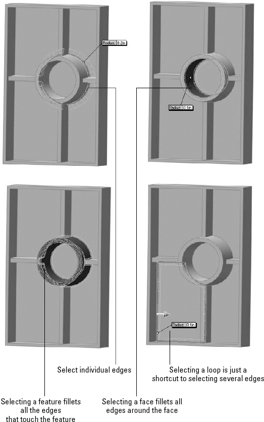
You can create fillets from several selections, including edges, faces, features, and loops. Edges offer the most direct method, and are the easiest to control. Figure 7.30 shows how you can use each of these selections to create fillets on parts more intelligently.
Tip
To select features for filleting, you must select them from the FeatureManager. The Selection Filter only filters edges and faces for fillet selection. You can select loops in two ways: through the right-click Select Loop option, or by selecting a face and Ctrl+selecting an edge on the face.
Another option for selecting edges in the Fillet command is the Select Through Faces option, which appears on the Fillet Options panel. This option enables you to select edges that are hidden by the model. This can be a useful option on a part with few hidden edges, or a detrimental option on a part where there are many edges due to patterns, ribs, vents, or existing fillets. You can control a similar option globally for features other than fillets by choosing Tools
Faces and Features selections are useful when you are creating fillets where you want the selections to update. In Figure 7.31, the ribs that are intersecting the circular boss are also being filleted. If the rib did not exist when the fillet was applied, but was added later and reordered so that it came before the Fillet feature; then the fillet selection automatically considers the rib. If the fillet used edge selection, this automatic selection updating would not have taken place.
By default, fillets have the Tangent Propagation option turned on. This is usually a good choice, although there may be times when you want to experiment with turning it off. Tangent propagation simply means that if you select an edge to fillet, and this edge is tangent to other edges, then the fillet will keep going along tangent edges until it forms a closed loop, the tangent edges stop, or the fillet fails.
If you deselect Tangent Propagation, but there are still tangent edges, you may see different results. One possible result is that it could fail. One of the tricks with fillet features is to try to envision what you are asking the software to do. For example, if one edge is filleted and the next edge is not, then how is the fillet going to end? Figure 7.31 shows two of the potential results when fillets are asked not to propagate. The fillet face may continue along its path until it runs off the part or until the feature fails.
Tip
This may sound counterintuitive, but sometimes when fillet features fail, it may be useful to deselect propagation and make the fillet in multiple features. There are times when creating two fillets like the one shown in Figure 7.31 will work, and making the same geometry as a single feature will not. This may be due to geometry problems where the sharp edges come together and are eliminated by the fillet.
Best Practice
In general, fillets should be the last features that are applied to a model, particularly the small cosmetic or edge break fillets. Larger fillets that contribute to the structure or overall shape of the part may be applied earlier.
Be careful of the rock-paper-scissors game that you inevitably are caught up in when modeling plastic parts and deciding on the feature order of fillets, draft, and shell. Most fillets should come after draft, and large fillets should come before the shell. Draft may come either before or after the shell, depending on the needs of the area that you are dealing with on the part. In short, there is no single set of rules that you can consistently apply and that works best in all situations.
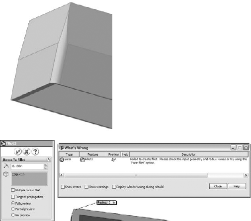
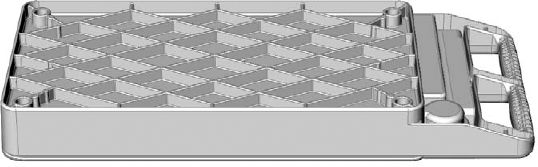
Figure 7.32 shows a model with a bit of a filleting nightmare. This large plastic tray requires many ribs underneath for strength. Because the ribs may be touched by the user, the sharp edges need to be rounded. Interior edges need to be rounded also for strength and plastic flow through the ribs. Literally hundreds of edges would need to be selected to create the fillets if you do not use an advanced technique.
Some of the techniques outlined previously, such as face and feature selection, can be useful for quickly filleting a large number of edges. Another method that still selects a large number of edges, but is not as intuitive as the others, is window selection of the edges. To use this option effectively, you may want to first position the model into a view where only the correct edges will be selected, turn off the Select Through Faces option, and use the Edges Selection filter.
The FilletXpert is a tool with several uses. One of the functions is its capability to select multiple edges. A part like the one shown in Figure 7.32 is ideal for this tool. To use the FilletXpert, click the FilletXpert button in the Fillet PropertyManager. Figure 7.33 shows this. When you select an edge, the FilletXpert presents a pop-up tool bar giving you a choice of several selection options. Notice that Figure 7.33 shows the majority of the edges selected that are needed for this fillet.
The FilletXpert is also a tool that automatically finds solutions to complex fillet problems, particularly when you have several fillets of different sizes coming together.
The Corner tab of the FilletXpert enables you to select from different corner options, which are usually the result of different fillet orders. To use the CornerXpert, make sure the FilletXpert is active; then click on the corner face, and toggle through the options.
I like to use the fillet preview. It helps to see what the fillet will look like, and perhaps more important, the presence of a preview usually (but not always) means that the fillet will work.
Unfortunately, when you have a large number of fillets to create, the preview can cause a significant slowdown. Deselecting and using the Partial Preview are both possible options. Partial Preview shows the fillet on only one edge in the selection and is much faster when you are creating a large number of fillets.
Performance
For rebuild speed efficiency, you should make fillets in a minimum number of features. For example, if you have 100 edges to fillet, it is better for performance to do it with a single fillet feature that has 100 edges selected rather than 100 fillet features that have one edge selected. This is the one case where creating the feature and rebuilding the feature are both faster by choosing a particular technique. (Usually if it is faster to create, it rebuilds more slowly.)
Best Practice
Although creation and rebuild speed are in sync when you use the minimum number of features to create the maximum number of fillets, this is not usually the case. (There had to be a downside.) When a single feature has a large selection, any one of these edges that fail to fillet will cause the entire feature to fail. As a result, a feature with 100 edges selected is 100 times more likely to fail than a feature with a single edge. Large selection sets are also far more difficult to troubleshoot when they fail than small selection sets that fail.
When you have a large number of fillet features, it can be tedious to navigate the FeatureManager. Therefore, it is useful to place groups of fillets into folders. This makes it easy to suppress or unsuppress all the fillets in the folder at once. Separate folders can be particularly useful if the fillets have different uses, such as fillets that are used for PhotoWorks models and fillets that are removed for FEA (Finite Element Analysis) or drawings.
The Multiple Radius Fillet option in the Fillet PropertyManager enables you to make multiple fillet sizes within a single fillet feature. Figure 7.34 shows how the multiple radius Fillet feature looks when you are working with it. You can change values in the callout flags or in the PropertyManager.

This may seem like an attractive way to group several fillets into as small a space on the FeatureManager as possible, but I cannot think of a single reason that would drive me to use this option. While there may be a small performance benefit to condensing several features into one, many more downsides adversely affect performance:
Loss of control of feature order.
A single failed fillet causes the whole feature, and thus all the fillets, to fail.
Troubleshooting is far more difficult.
Smaller groups of fillets cannot be suppressed without suppressing everything.
You cannot change the size of a group of fillets together.
Best Practice
While this may be more personal opinion than best practice, I believe that there are good reasons to consider using techniques other than single features that contain many fillets, or single features that drive fillets of various sizes. Best practice would lean more toward grouping fillets that have a similar use and the same size. For example, you may want to separate fillets that break corners on ribs from fillets that round the outer shape of a large plastic part.
Another consideration is feature order when it comes to the fillet's relationship to draft and shell features. If the fillets are all grouped into a single feature, then controlling this relationship becomes impossible.
The Round corners option refers to how SolidWorks handles fillets that go around sharp corners. By default, this setting is off, which leaves fillets around sharp corners looking like mitered picture frames. If you turn this setting on, the corner looks like a marble has rolled around it. Figure 7.35 shows the resulting geometry from both settings.

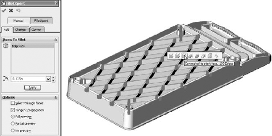
The Keep edge/Keep surface toggle determines what SolidWorks should do if a fillet is too big to fit in an area. The Keep Edge option keeps the edge where it is and tweaks the position (not the radius) of the fillet to make it meet the edge. The Keep surface option keeps the surfaces of the fillet and the end face clean; however, to do this, it has to tweak the edge. There is often a tradeoff when you try to place fillets into a space that is too small. Sometimes it is useful to try to visualize what you think the result should look like. Figure 7.36 shows how the fillet would look in a perfect world, followed by how the fillet looks when cramped with the Keep edge option and how it looks when cramped with the Keep surface option.
The Default option chooses the best option for a particular situation. As a result, it seems to use the Keep edge option unless it does not work, in which case it changes to the Keep surface option.
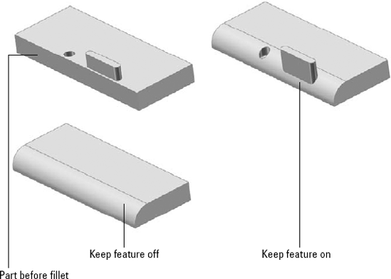
The Keep Feature option appears on the Fillet Options panel of the Fillet PropertyManager. By default, this option is turned on. If a fillet surrounds a feature such as a hole (as long as it is not a through hole) or a boss, then deselecting the Keep Feature option removes the hole or boss. When Keep Feature is selected, the faces of the feature trim or extend to match the fillet, as shown in Figure 7.37.
Variable radius fillets are another powerful weapon in the fight against boring designs; they also double as a useful tool to solve certain problems that arise. Although it is difficult to define exactly when to use the variable radius fillet, you can use it when you need a fillet to round an edge, and it has to change in size to fit the available geometry.
Best Practice
It may be easier to identify when not to use a variable radius fillet. Fillets are generally used to round or break edges, not to sculpt a part. If you are using fillets to sculpt blocky parts and are not actively trying to make blocky parts with big fillets, you may want to consider another approach and use complex modeling, which gives the part a better shape and makes it more controllable. Other options exist that give you a different type of control, such as the double hold line fillet.
In some ways, variable radius fillets function like other fillets. For example, they offer propagation to tangent edges and preview options.
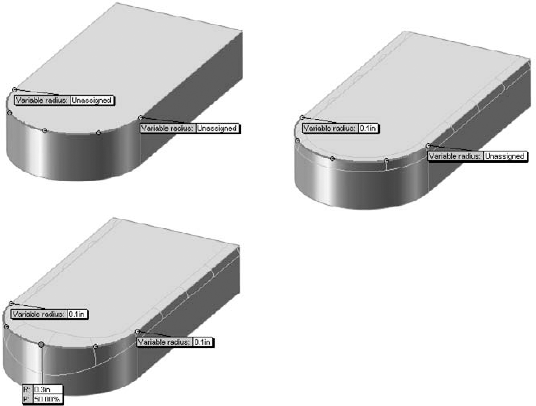
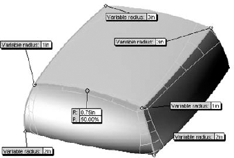
When you first select an edge for the variable radius fillet, the endpoints are identified by callout flags with the value unassigned. A preview does not display until at least one of the points has a radius value in the box. You can also apply radius values in the PropertyManager, but they are easier to keep track of using the callouts. Figure 7.38 shows a variable radius fillet after the edge selection, after one value has been applied, and after three values have been applied. To apply a radius value that is not at the endpoint of an edge, you can select one of the three colored dots along the selected edge. The preview should show you how the fillet will look in wireframe display.
By default, the variable radius fillet puts five points on an edge, one at each endpoint, one at the midpoint, and one each halfway between the ends and middle. If you want to create an additional control point, there are three ways to do it:
Ctrl+drag an existing point
Select the callout of an existing point and change the P (percentage) value
Change the Number of Instances value in the Variable Radius Parameters panel of the PropertyManager
If you have selected several edges, and several unassigned values are on the screen, then you can use the Set Unassigned option in the PropertyManager to set them all to the same value. The Set All option sets all radius values to the same number, including any values that you may have changed to be different than the rest. Figure 7.39 shows the Variable Radius Parameters panel.

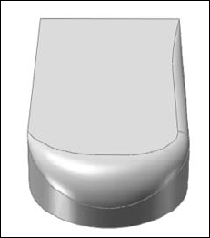
Another available option with the variable radius fillet is that you can set a value of zero at an end of the fillet. You need to be careful about using a zero radius, because it is likely to cause downstream problems with other fillets, shells, offsets, and even machining operations. You cannot assign a zero radius in the middle of an edge, only at the end. If you need to end a fillet at a particular location, you can use a split line to split the edge and apply a zero radius at that point. Figure 7.40 shows a part with two zero-radius values.
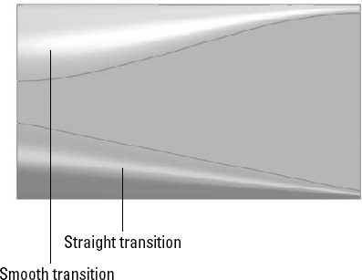
Variable radius fillets have an option for either a straight transition or a smooth transition. This works like the two-profile lofts that were mentioned earlier in this chapter. The names may be somewhat misleading because both transitions are smooth. The straight transition goes in a straight line, from one size to the next, and the smooth transition takes a swooping S-shaped path between the sizes. The difference between these two transitions is demonstrated in Figure 7.41.
Variable radius fillets use a different method to create the fillet geometry than the default constant radius fillet. Sometimes using a variable radius fillet can make a difference where a constant radius fillet does not work. This is sometimes true even when the variable radius fillet uses constant radius values. It is just another tool in the toolbox.
Face Fillets may be the most flexible type of fillet because of the range of what they can do. Face Fillets start as simply an alternate selection technique for a constant radius fillet and extend to the extremely flexible double hold line face fillet, which is more of a blend than a fillet.
Under normal circumstances, the default fillet type uses the selection of an edge to create the fillet. An edge is used because it represents the intersection between two faces. However, there can sometimes be a problem with the edge not being clean or being broken up into smaller pieces, or any number of other reasons causing a constant radius fillet using an edge selection to fail. In cases like this, SolidWorks displays the error message, "Failed to create fillet. Please check the input geometry and radius values or try using the 'Face Fillet' option."
Users almost universally ignore these messages. In the situation shown in Figure 7.42, the Face Fillet option suggested in the error message is exactly the one that you should use. Here the face fillet covers over all the junk on the edge that prevents the fillet from executing.

Face Fillets are sometimes amazing at covering over a mess of geometry that you might think you could never fillet. The main limitation on fillets of this type is that the fillet must be big enough to bridge the gap. That's right, I said big enough. Face Fillets can fail if they are either too small or too large. Figure 7.43 shows a complex fillet situation that is completely covered by a face fillet.
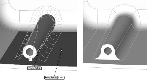
On the CD-ROM
The model used for this image can be found on the CD-ROM, with the filename Chapter 7 Plastic Cover Fillets.sldprt.
Curvature continuity refers to the quality of a transition between two curves or faces, where the curvature is the same or continuous at and around the transition. The best way to convey this concept is with simple 2D sketch elements. When a line transitions to an arc, you have non-continuous curvature. The line has no curvature, and there is an abrupt change because the arc has a specific radius.
Note
Radius is the inverse of curvature, and so r = 1/c. For a straight line, r = ∞, in which case c = 0.
To make the transition from r = ∞ to r = 2 smoothly, you would need to use a variable radius arc if such a thing existed. There are several types of sketch geometry that have variable curvature, such as ellipses, parabolas, and splines. Ellipses and parabolas follow specific mathematical formulas to create the shape, but the spline is a general curve that can take on any shape that you want, and you can control its curvature to change smoothly or continuously. Splines, by their very definition, have continuous curvature within the spline, although you cannot control the specific curvature or radius values directly.
All this means that continuous curvature Face Fillets use a spline-based variable-radius section for the fillet, rather than an arc-based constant radius. Figure 7.44 illustrates the difference between continuous curvature and constant curvature. The spikes on top of the curves represent the curvature (1/r, and so the smaller the radius, the taller the spike). These spikes are called a curvature comb.
In Comparison to Figure 7.45, notice how the curvature comb immediately jumps from no curvature to the constant arc radius, but the spline image ramps up to a curvature that varies.
The Help Point in the Face Fillet PropertyManager is a fairly obscure option. However, it is useful in cases where the selection of two faces does not uniquely identify an edge to fillet. For example, Figure 7.45 shows a situation where the selection of two faces could result in either one edge or the other being filleted (normally, I would hope that both edges would be filleted). The fillet will default to one edge or the other, but you can force it to a definite edge using the Help Point.
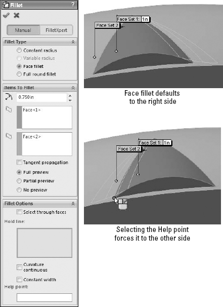
In some cases, the Help Point is ignored altogether. For example, if you have a simple box, and select both ends of the box as selection set 1, and the top of the box as selection set 2, then the fillet could go to either end. Consequently, assigning a Help Point will not do anything in this case, because multiple faces have been selected. The determining factor is which of the multiple faces is selected first. If this were a more commonly used feature, the interface for it might be made a little less cryptic, but because this feature is rarely, if ever, used, it just becomes a quirky piece of trivia.
A single hold line fillet is a form of variable radius fillet, but instead of it being defined using the variable radius fillet type, it is created using the face fillet. Rather than the radius being driven by specific numerical values, it is driven by a hold line, or edge, on the model. The hold line can be an existing edge, forcing the fillet right up to the edge of the part, or it can be created by a split line, which enables you to drive the fillet however you like. Figure 7.46 shows these two options, before and after the fillets. Notice that these fillets are still arc-based fillets; if you were to take a cross-section perpendicular to the edge between filleted faces, it would be an arc cross-section with a distinct radius. However, in the other direction, hold line fillets do not necessarily have a constant radius, although they may if the hold line is parallel with the edge between faces.

You can select the Hold line in the Fillet Options panel of the Face Fillet PropertyManager, as shown in Figure 7.47. The top panel, Fillet Type, is available only when the feature is first created. When you edit it after it has been created, the Fillet Type panel does not appear. As a result, you cannot change from one top-level type of fillet to another after it has been initially created.
There are times when a single hold line does not meet your needs. The single hold line controls only one side of the fillet, and in order to control both sides of the fillet, you must use a double hold line fillet. SolidWorks software does not specifically differentiate between the single and double hold line fillets, but they are radically different in how they create the geometry. When both sides of the fillet are controlled, it is not possible to span between the hold lines with an arc that is tangent to both sides unless you were careful about setting up the hold lines so that they are equidistant from the edge where the faces intersect. This means that the double hold line fillet must use a spline to span between hold lines, as shown in Figure 7.48.

To get this feature to work, you need to use the curvature continuous option in the Fillet Options panel. Remember that this option creates a spline-based fillet rather than an arc-based fillet, which is exactly what you need for a double hold line fillet. This makes the double hold line fillet more of a blend than a true fillet. Figure 7.49 shows examples of the double hold line fillet.
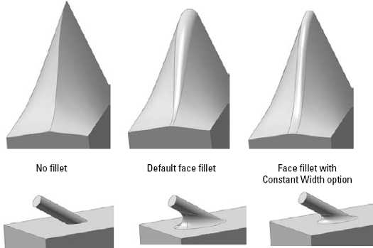
The Constant width option of the Face Fillet PropertyManager drives a fillet by its width rather than by its radius. This is most helpful on parts where the angle of the faces between which you are filleting is changing dramatically. Figure 7.50 illustrates two situations where this is particularly useful. The setting for constant width is found in the Options panel of the Face Fillet PropertyManager. The part shown in the images is on the CD-ROM as Chapter 7 Constant Width.sldprt.

The full round fillet is very useful in many situations. In fact, it may actually work in situations where you would not expect it to. It does require quite a bit of effort to accomplish the selection, but it compensates by enabling you to avoid alternate fillet techniques.
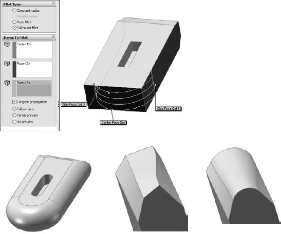
To create a full round fillet, you have to select three sets of faces. Usually one face in each set is sufficient. The fillet is tangent to all three sets of faces, but the middle set is on the end and the face is completely eliminated. Figure 7.51 shows several applications of the full round fillet. Notice that it is not limited to faces of a square block, but also propagates around tangent entities and can create a variable radius fillet over irregular lofted geometry.
The setback fillet is the most complex of the fillet options. You can use the Setback option in conjunction with constant radius, multiple radius, and variable radius fillet types. A setback fillet blends several fillets together at a single vertex, starting the blend at some "setback" distance along each filleted edge from the vertex. At least three, and often more, edges come together at the setback vertex. Figure 7.52 shows the PropertyManager interface and what a finished setback fillet looks like. The following steps demonstrate how to use the setback fillet.

Setting up a setback fillet can take some time, especially if you are just learning about this feature. You must specify values for fillet radiuses, select edges and vertices, and specify six setback distances. If you are using multiple radius fillets or variable radius fillets, then this becomes an even larger task. The steps are as follows:
Determine the type of fillet to be used:
Constant radius fillet
Multiple radius fillet
Variable radius fillet
Select the edges to be filleted. Selected edges must all touch one of the setback vertices that will be selected in a later step.
Assign radius values for the filleted items. Figure 7.53 shows a sample part that illustrates this step.

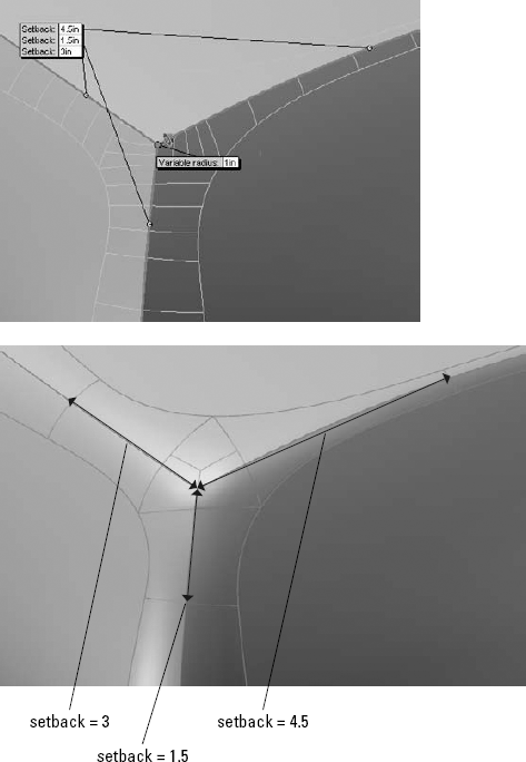
Enter setback values. As shown in Figure 7.54, the setback callout flags have leaders that point from a specific value to a specific edge. The dimensions refer to distances, as shown in the image to the right in Figure 7.54. The setback distance is the distance over which the fillet will blend from the corner to the fillet.
Warning
When you select multiple vertices, the preview arrows that indicate which edge you are currently setting the setback value for may be incorrect. The arrows can only be shown on one vertex; therefore, you may want to rely on the leaders from the callouts to determine which setback distance you are currently setting.
Repeat the process for all selected setback vertices. If you are using a preview, then you may notice that the preview goes away when starting a second set of setback values. Don't worry. This is probably not because the feature is going to fail. Once you finish typing the values, the preview will return. When you have spent as much time setting up a feature as you will spend on this, seeing the preview disappear can be frustrating; however, persevere, and it will return.
SolidWorks contains several specialty features that perform tasks that you will use less often. Although you will not use these features as frequently as others, you should still be aware of them and what they do, because you never know when you will need them.
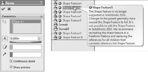
Until SolidWorks 2010, another very similar feature existed, which was called Shape. You can no longer make Shape features, but you may find one from time to time in old parts. If you find a Shape feature on an old part, it will continue to function unless any of its parent geometry changes. Shape features will not update in SolidWorks 2010 or later. SolidWorks recommends you re-create the geometry as another feature, possibly a Dome or Freeform feature.
Best Practice
Dome features are best used when you are looking for a generic bulge or indentation, and are not too concerned about controlling the specific shape. Occasionally, a dome may be exactly what you need, but when you need more precise, predictable control, then you should use the Fill, Boundary, or Loft feature.
The Dome feature has several attributes that will either help it qualify for a given task, or disqualify it. These attributes can help you decide if it will be useful in situations you encounter:
The Dome feature can create multiple domes on multiple selected faces in a single feature, although it creates only a single dome for each face.
Using the Elliptical Dome setting, Dome can create a feature that is tangent to the vertical.
Dome can use a constraint sketch to limit its shape.
Dome works on non-planar faces.
Dome cannot establish a tangent relationship to faces bordering the selected face.
Dome cannot span multiple faces.
Dome displays a temporary untrimmed four-sided patch that extends beyond the selected face when you use it on a non-four-sided face.
Dome functions only on solids, not on surfaces.
The error caused by a Shape feature being forced to update in SolidWorks 2010 is shown in Figure 7.55.
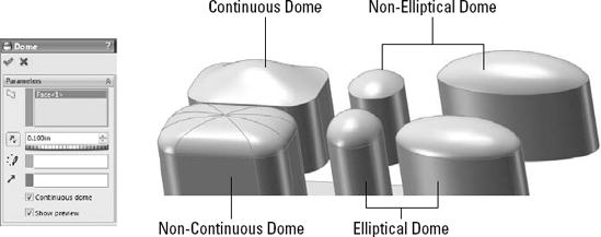
The Dome feature has two notable settings: the Elliptical Dome and Continuous Dome.
The Elliptical Dome is available only on flat faces where the boundary is either a complete circle or an ellipse. The cross-section of the dome is elliptical, and does not account for draft, which means that it is always tangent to the perpendicular from the selected flat face.
The Continuous Dome is a setting for any non-circular or elliptical face, including polygons and closed-loop splines. The setting results in a single unbroken face. If you deselect the Continuous Dome setting, it functions like the Elliptical Dome setting. Figure 7.56 shows the most useful settings for the Dome feature.
The Wrap feature works by flattening the face, relating the sketch to the flat pattern of the face, and then mapping the face boundaries and sketch back onto the 3D face. The reason why it is limited to cylindrical and conical faces is that these types of geometry are developable. This means that the faces can be mapped to the flat pattern through some relatively simple techniques that happen behind the scenes. Developable geometry can be flattened without stretching. You will see in a later chapter that sheet metal functions are limited in the same way and for the same reasons.
SolidWorks does not wrap onto other types of surfaces, such as spherical, toroidal, or general NURBS surfaces, because you cannot flatten these shapes without distorting or stretching the material. There is software that can flatten these shapes, but it is typically done for sheet-metal deep drawing applications, which highly deform the metal. Figure 7.57 shows the Wrap PropertyManager interface.
The Wrap feature has three main options:
Emboss
Deboss
Scribe

Scribe is the simplest of the options to explain, and understanding it can help you understand the other options. Scribe creates a split line-like edge on the face.
Several requirements must be met in order to make a wrap feature work:
The face must be a cylindrical or conical face.
The loop must be a closed loop or nested closed loop 2D sketch.
The sketch must be on a plane that is either tangent to or parallel to another plane that is tangent to the face.
Wrap supports multiple closed loops within a single feature.
Wrap supports wrapping onto multiple faces.
The wrap should not be self-intersecting when it wraps around the part. (Self-intersection will not cause the feature to fail, but on the other types, Emboss and Deboss, it may produce unexpected results.)
Scribes can be created on solid or surface faces. Scribed surfaces are frequently thickened to create a boss or a cut.
The Wrap Emboss option works much like the scribe, but it adds material inside the closed loop sketch, at the thickness that you specify in the Emboss PropertyManager. Embossing can only be done on solid geometry. If the feature self-intersects, then the intersecting area is simply not embossed, and is left at the level of the original face. One result is that creating a full wrap-around feature, such as the geometry for a barrel cam, requires a secondary feature. This is because the Wrap feature always leaves a gap, regardless of whether the sketch to be wrapped is under or over the diameter-multiplied-by-pi length.
Tip
To work around this problem, you can use a loft, extrude, or revolve feature to span the gap.
When you use the Emboss option, you can set up the direction of pull and assign draft so that the feature can be injection molded. This limits the size of the emboss so that it must not wrap more than 180 degrees around the part.
Deboss is just like emboss, except that it removes material instead of adding it. Figure 7.58 demonstrates all these options. The part shown in the images is available on the CD-ROM with the filename Chapter 7 Wrap.sldprt. For each of the demonstrated cases, the original flat sketch is shown to give you some idea of how the sketch relates to the finished geometry.
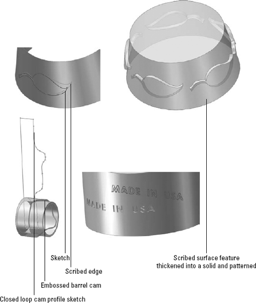
Keep in mind that this feature is not like the projected sketch. A projected sketch is not foreshortened on the curved surface, but is projected normal from the sketch plane. A sketch that is one-inch long will measure one-inch along the curvature of the surface and will measure less than one inch linearly from end to end.
The scribed part in the previous figure was created on a conical surface body. The surface was then thickened as a separate body and patterned.
Cross-Reference
Chapter 26 covers working with multi-bodies, and Chapter 27 covers surfaces.
The embossed cam employed a workaround with a revolve feature to close the gap that is always created when wrapping all the way around a part.
The example with the debossed text employs a direction of pull and draft so that the geometry can be molded.
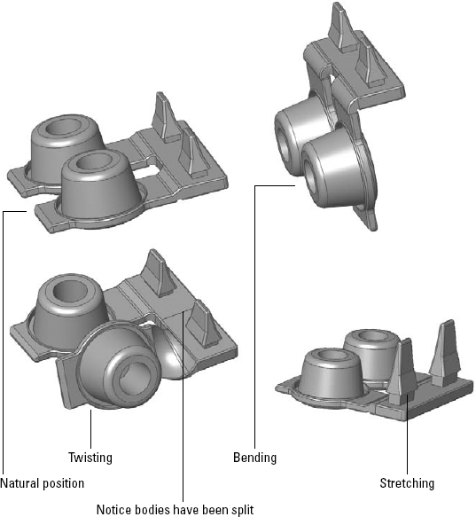
Figure 7.59 shows the Flex PropertyManager interface. Flex has four main options and many settings. The four main options are as follows:
Bending. Establishes two trim planes to denote the ends of the bent area, and specifies an angle or radius for the bend.
Twisting. Establishes two trim planes to limit the area of the twist, and enters the number of degrees through which to twist.
Tapering. Establishes two trim planes to limit the area of the taper. The body will be larger toward one end and smaller toward the other end.
Stretching. Establishes two trim planes to limit the area to be stretched. You can stretch the entire body by moving the trim planes outside of the body.
Best Practice
Flex is not the kind of feature that you should use to actually design parts, but it can be extremely valuable when you need to show a part in an "in use" state. A simple example would be a rubber strap that stretches over something when it is used, but that is designed and manufactured in its free state. The geometry that you can create by using the flex functions is not generally production-model quality, but it is usually adequate for a looks-like model.
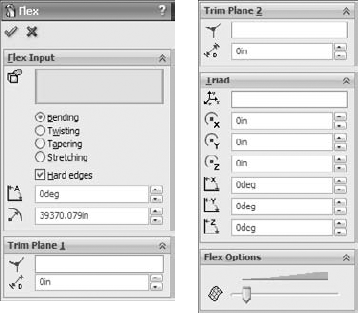
Figure 7.60 shows examples of each flex option using a model of a rubber grommet. The part shown in the figure can be found on the CD-ROM with the filename Chapter 7 Flex.sldprt.
In some cases, the triad and trim planes are slightly disoriented. The best thing to do in situations like this is to simply reorient the triad using the angle numbers in the Triad panel of the PropertyManager. This is also a solution if the planes are turned in such a way that the axis of bending is not oriented to the bend that the part requires.
The Flex feature is very conscious of separate bodies. In some cases this can be helpful, but in default situations when there is only one body in the part, it can be annoying. Remember to select the body to be affected in the very first selection box at the top of the PropertyManager.
Tip
If you want to bend only one of the tabs on the grommet, then the best solution is to split the single body into two bodies and flex only one of the bodies. The examples shown for twisting and stretching use this technique.
Cross-Reference
Splitting a single body into multiple bodies is covered in Chapter 26.
You can place the trim planes by selecting a model vertex, by dragging the arrow on the plane, or by typing in a number. Be careful when dragging the plane arrows because dragging the border of the plane drags the flex value for the feature. (Dragging the plane in a bending operation is like changing the angle or radius for the bend.)
Using the triad can be very tricky. Moving the triad in the bending option moves the axis of the bend, and so it determines whether the bend will compress or stretch the material. The position of the triad also determines which side of the bent body will move or stay stationary, or if both sides will move. Placing the triad directly on a trim plane causes the material outside the bend on that side of the trim plane to remain stationary.
I highly recommend taking a look at the models that are provided with this chapter to examine the various functions of the Flex feature more carefully. The model uses configurations, which are covered in Chapter 10.
The Deform feature is also another feature type that you may not use to actually design anything, but that you may use to show a model in a deformed state.
Also, it is a minor point, but if you use the large icons setting, notice that the toolbar icon used for Deform is the wrong one. The icon used for large icons is the Boundary Cut icon. Just be careful if you use large icons.
Best Practice
Typically, if you want a model to have a certain shape, then you need to intentionally and precisely model it with that shape. The problem with using deform and flex geometry for actual design data is that they both create fairly approximate geometry, and this process yields a result that is not completely intentional. The shape that you finally achieve is the result of arbitrary uncontrolled function of the feature, not necessarily creating a shape that you had clearly envisioned beforehand.
Deform has three types:
Point. This type deforms a portion of the model by pushing a point and the geometry around it.
Curve to curve. The most precise and useful deform type, this type selects an existing edge and forces the edge to match a curve.
Surface push. This type of deform, while conceptually a very interesting function, is nearly unusable in practice. The part is deformed into a shape vaguely resembling an intermediate shape between the existing state of the part and a "tool" body.
Figure 7.61 shows the PropertyManager interface for the Deform feature. The interface is different for each of the three main types, and also changes, depending on selections within the individual types. The interface shown is for the Curve to curve type because I believe this to be the most useful type.
The Point deform option enables you to push a point on the model, and the model deforms as if it were rubber. Figure 7.62 shows the PropertyManager, as well as a before-and-after example of the Point deform function. The key to using this feature is to ensure that the Deform region option is unselected. Aside from that, you just have to use trial and error when applying the Point deform option. The depth, diameter, and shape of the deformation are not very precise. Also, you cannot specify the precise location for the point to be deformed. Again, this is best used for "looks-like" models, not production data.
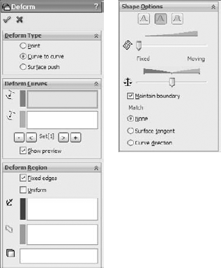

In the model from Figure 7.62, two Point deform features are used, one to apply some shape to the back and one to apply some shape to the seat.
Because the Curve to curve uses curve (or sketch or edge) data, it is a more precise method than the other deform types. The main concept here is to transform a curve on the original model to a new curve, thus deforming the body to achieve the new geometry.
The model shown in Figure 7.63 has been created using the Curve to curve deform. The part starts as a simple sweep (sweep an arc along an arc), and then a split line is created to limit the deform to a specific area of the model. The model is on the CD-ROM with the filename Chapter 7 Deform Curve to Curve.sldprt.

I do not go into much detail on the Surface push deform type because it is not one of the more useful functions in SolidWorks. In order to use it, you must have the body of the part that you are modeling, and a tool body that you will use to shape the part that you are modeling. The finished shape does not fit the tool body directly, but looks about half-way between the model and the tool body, blended together in an abstract sort of way. It looks like the dent that would result from an object being thrown very hard at a car fender, in that neither the thrown part nor the fender is immediately recognizable from the result.
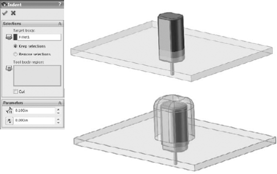
In this case, the small motor is placed where it needs to be, but there is a wall in the way. Indent is used to create an indentation in the wall by using the same wall thickness and placing a gap of .010 inches around the motor. The motor is brought into the wall part using the Insert
When you follow this tutorial, you are encouraged to follow the directions the first time to make sure that you understand the concepts involved, and then to go through it again, this time deviating from the instructions to see if you can expand your understanding by experimentation. To try bracket casting, follow these steps:
Open a new part using an inch-based template.
On the Right plane, draw a circle centered at the origin with a diameter of 1.50 inches, and a second circle placed 4.000 inches vertically from the first, with a diameter of 2.250 inches.
Exit the sketch, and make sure Instant 3D is selected. The Instant 3D icon is on the Features toolbar, and looks like a ruler with an arrow. Click on the sketch in the graphics window, and pull the Instant 3D arrow to create a solid. Edit the feature (right- or left-click the feature either in the graphics window or in the FeatureManager and click the Edit Feature icon, which is the yellow and green block with a hand pointing to it). Now enter numbers by hand so that you extrude the sketch 1.000 inch using a From condition of Offset by 1.000 inch, such that the offset and the extrude depth are in the same direction. Rename this feature Bosses in the FeatureManager. Figure 7.65 shows the results of these steps.

Note
These steps produce multiple bodies that will be merged in a later step. Multi-body parts are covered in more detail in Chapter 26. You can tell that there are multiple bodies by looking at the Solid Bodies folder near the top of the tree and expanding the folder. The bodies are listed in the folder.
On the Top plane, open a new sketch and draw a horizontal construction line across the cylinder, from the midpoint of one side to the midpoint of the other side. To pick up the automatic relations for the midpoints more easily, it is recommended that you orient the view, normal to the sketch, or use the Top view. It does not matter if you make the relations to the top or bottom cylinder, because the midpoints of the sides are in the same place when they are projected into the sketch plane.
Next, draw an ellipse (Tools
Sketch Tools Ellipse) centered at the midpoint of the construction line and that measures .700 inches horizontally and 1.375 inches vertically. You may want to assign a relation between the center of the ellipse and one of the control points to prevent the ellipse from rotating and fully define the sketch Exit the sketch when you are satisfied with the result.
Show the sketch for the Bosses feature. (Click the plus icon next to the Bosses extrude to show the sketch, and then right-click the sketch and select Show.)
Create a plane parallel to the Top plane at the center of the larger circle. You can access the Plane creation interface by choosing Insert
Draw a second ellipse on the Top Boss Plane. Do not draw a construction line as you did for the first ellipse; instead, you can just make the centerpoint of the second ellipse directly on top of the first ellipse's centerpoint. The dimensions should be 1.000 inch horizontal by 1.750 inches vertical. Figure 7.66 shows the results up to this point.
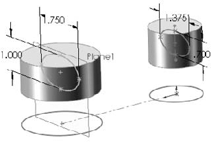
Tip
When you are sketching on parallel planes that are separated by some distance and trying to pick up automatic relations, it is often very helpful to be looking "normal to" the sketch, so that you can see how other entities are projected into the sketch plane.
Use the Loft feature to loft between the two ellipses. Be sure to select the ellipses in approximately the same location so that they do not twist. If the loft preview accidentally twists, then use the connectors (light-blue square dots on the sketches that are connected by a straight line) to straighten out the loft.
Note
Notice that this feature joined together the other two disjoint bodies with the body that was created by the loft into a single body. This is a result of selecting the Merge Result option in the Options panel.
Tip
If you want to experiment, expand the Start/End Constraints panel and apply end conditions for the loft. This causes the loft to change from a straight loft to a curved loft.
Right-click all sketches that are showing, and select Hide. Do the same for the Top Boss Plane. This cleans up the display to prevent it from becoming confusing. However, if you prefer to see the sketches, then you can leave them displayed.
Tip
You can either hide or show different types of entities in groups by using the View menu. Hide All Types hides everything, and disables the options for individual entity types to be used.
Open a sketch on the Right plane. Sketch an ellipse such that the center is oriented 1.750 inches vertically from the Origin, and the ellipse measures .750 inches horizontally and 1.500 inches vertically.
Extrude this ellipse using the Up To Next end condition. If Up To Next does not appear in the list, then change the direction of the extrude and try it again.
Show the sketch of the Bosses feature by expanding the feature (click the "+" next to it), right- or left-clicking the sketch icon, and clicking the Hide/Show icon (eyeglasses). Next, open a sketch on the Right plane. Sketch two circles that are concentric with the original circles, with the dimensions of .875 inches and 1.250 inches. Exit the sketch.
Use Instant 3D to create an extruded cut that goes through the large circular bosses. This feature will look like a boss extrusion at first, so when you have finished dragging its depth, a small toolbar with two icons appears. One of the icons enables you to add draft; the other enables you to turn the boss into a cut. Figure 7.67 shows the state of the model up to this step.
Start a fillet feature, and select the face of the Loft feature. Assign a radius of .200 inches.
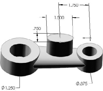
Note
Although this fillet is created by selecting a face, it is not a face fillet. Selecting a face for a regular constant radius fillet simply fillets any edge that is on the face.
Create a mirror feature, using the Right plane as the mirror plane. In the Mirror PropertyManager, expand the Bodies To Mirror panel, and select anywhere on the part. Make sure that the Merge Solids option is selected. Click OK to accept the mirror.
Orient the view to the Front view, and then turn the view on its side (hold down Alt and press the left- or right-arrow key six times).
Open a new sketch on the Front plane. From the View menu, make sure that Hide All Types is not selected, and show Temporary Axes. Draw and dimension a horizontal construction line, as shown in Figure 7.68.
With the construction line selected, start the Sketch Text command (Tools
Sketch EntitiesText). Make sure that the line appears in the Curves selection box.Click in the text box, and type Made in USA (or your name or company name). Select the text and click the Bold button. Deselect the Use Document Font option, change the font to use units, and set the height to .175 inches.
Click OK to exit the Sketch Text PropertyManager, and click OK again to exit the sketch. You can turn off the Temporary Axis display.
Choose Insert
FeaturesWrap. You should be prompted to select a plane or a sketch. Use the Flyout FeatureManager to select the sketch that you just created with the sketch text in it. Next, select the cylindrical face of the boss to see a preview of the text wrapped onto the face. If the text appears backward, then select the Reverse Direction option in the Wrap PropertyManager.Select the Emboss option, and assign a thickness of .025 inches. Click in the Pull Direction selection box and select the Front plane. Click OK to accept the feature.
Save the part and close it. If you would like to examine the reference part, you can find it on the CD-ROM with the filename Chapter 7
Tutorial Bracket Casting.sldprt. The finished part is shown in Figure 7.69.


Follow these steps to create a wire-formed part:
Open a new part using an inch-based template.
Open a sketch on the Right plane and sketch a circle that is centered on the Origin with a diameter of 1.500 inches.
Create a Helix, Constant Pitch, Pitch, and Revolution, where the Pitch = .250 inches, Revolutions = 5.15, and Start Angle = 0. The Helix command is found at Insert
Create a sketch on the Front plane, as shown in Figure 7.70. Pay careful attention when adding the construction line, as shown. This line is used in the next step to reference the end of the arc.
Open a sketch on the Right plane and use Figure 7.71 to add the correct relations and dimensions. Be aware that the two sketches shown are on different sketch planes, which makes it difficult to depict in 2D. You can also open the part from the CD-ROM for reference.
Exit the sketch and create a projected curve. The Projected Curve function is found at Insert
Open a 3D sketch. You can access a 3D sketch from the Insert menu. Select the helix and click Convert Entities on the Sketch toolbar. Then select the projected curve and click Convert Entities again. You now have two sections of a 3D sketch that are unconnected in space.
Draw a two-point spline to join the ends of the 3D sketch entities that are closest to one another. Assign tangent relations to the ends to make the transition smooth. Figure 7.72 illustrates what the model should look like at this point.
Tip
You may have to adjust the length of one of the spline tangency length arrows to keep the spline from remaining inside the cylinder of the helix.
Open a sketch on the Right plane, and draw an arc that is centered on the Origin and coincident with the end of the 3D sketch helix. The 185-degree angle is created by activating the dimension tool and clicking first the center of the arc, and then the two endpoints of the arc. Now place the dimension. This type of dimensioning allows you to get an angle dimension without dimensioning to angled lines. Exit the sketch.
Create a Composite Curve (Insert
CurveComposite) consisting of the 3D sketch and the new 2D sketch.Create a new plane using the Normal to Curve option, selecting one end of the composite curve.
On the new plane, draw a circle that is centered on the end of the curve with a diameter of .120 inches. You need to create a Pierce relation between the center of the circle and the composite curve.
Create a sweep feature using the circle as the profile and the composite curve as the path. To create the sweep, you must first exit the sketch.
Hide any curves that still display.
Choose Insert
CutWith Surface. From the Flyout FeatureManager, select the Right plane. Make sure that the arrow is pointing to the side of the plane with the least amount of material. Click OK to accept the cut. The finished part is shown in Figure 7.73.

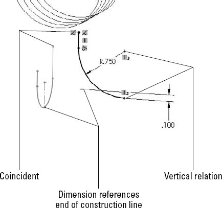
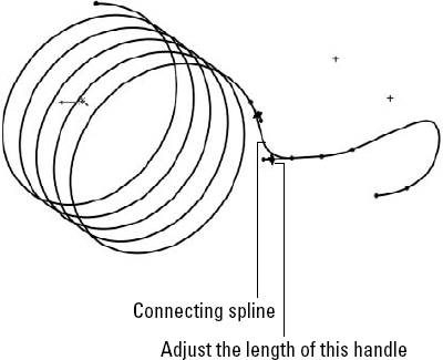
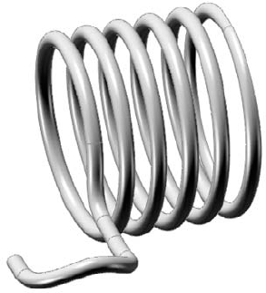
SolidWorks has a wide range of feature types to choose from, spanning from simple extrudes and revolves to more complex lofts and sweeps. It also offers a selection of specialty features that may not be useful on a day-to-day basis, but that have their place in the modeling techniques that you need to know to get the job done.
Some features, such as extrude, fillet, and flex, have so many options that it may be difficult to take them all in at once. You should browse through the models on the CD-ROM for this chapter and use the Rollback bar (described in detail in Chapter 11) to examine how the parts were built. You can then try to create a few on your own.