CHAPTER 1

INTRODUCTION

1.1 WHAT IS REGRESSION ANALYSIS?

Regression analysis is a conceptually simple method for investigating functional relationships among variables. A real estate appraiser may wish to relate the sale price of a home from selected physical characteristics of the building and taxes (local, school, county) paid on the building. We may wish to examine whether cigarette consumption is related to various socioeconomic and demographic variables such as age, education, income, and price of cigarettes. The relationship is expressed in the form of an equation or a model connecting the response or dependent variable and one or more explanatory or predictor variables. In the cigarette consumption example, the response variable is cigarette consumption (measured by the number of packs of cigarette sold in a given state on a per capita basis during a given year) and the explanatory or predictor variables are the various socioeconomic and demographic variables. In the real estate appraisal example, the response variable is the price of a home and the explanatory or predictor variables are the characteristics of the building and taxes paid on the building.

We denote the response variable by Y and the set of predictor variables by X₁, X₂,…, X_p, where p denotes the number of predictor variables. The true relationship between Y and X₁, X₂,…, X_p can be approximated by the regression model

where ε is assumed to be a random error representing the discrepancy in the approximation. It accounts for the failure of the model to fit the data exactly. The function f(X₁, X₂,…, X_p) describes the relationship between Y and X₁, X₂,…, X_p. An example is the linear regression model

where β₀, β₁,…, β_p, called the regression parameters or coefficients, are unknown constants to be determined (estimated) from the data. We follow the commonly used notational convention of denoting unknown parameters by Greek letters.

The predictor or explanatory variables are also called by other names such as independent variables, covariates, regressors, factors, and carriers. The name independent variable, though commonly used, is the least preferred, because in practice the predictor variables are rarely independent of each other.

1.2 PUBLICLY AVAILABLE DATA SETS

Regression analysis has numerous areas of applications. A partial list would include economics, finance, business, law, meteorology, medicine, biology, chemistry, engineering, physics, education, sports, history, sociology, and psychology. A few examples of such applications are given in Section 1.3. Regression analysis is learned most effectively by analyzing data that are of direct interest to the reader. We invite the readers to think about questions (in their own areas of work, research, or interest) that can be addressed using regression analysis. Readers should collect the relevant data and then apply the regression analysis techniques presented in this book to their own data. To help the reader locate real-life data, this section provides some sources and links to a wealth of data sets that are available for public use.

A number of datasets are available in books and on the Internet. The book by Hand et al. (1994) contains data sets from many fields. These data sets are small in size and are suitable for use as exercises. The book by Chatterjee, Handcock, and Simonoff (1995) provides numerous data sets from diverse fields. The data are included in a diskette that comes with the book and can also be found in the World Wide Web site.¹

Data sets are also available on the Internet at many other sites. Some of the Web sites given below allow the direct copying and pasting into the statistical package of choice, while others require downloading the data file and then importing them into a statistical package. Some of these sites also contain further links to yet other data sets or statistics-related Web sites.

The Data and Story Library (DASL, pronounced “dazzle”) is one of the most interesting sites that contains a number of data sets accompanied by the “story” or background associated with each data set. DASL is an online library² of data files and stories that illustrate the use of basic statistical methods. The data sets cover a wide variety of topics. DASL comes with a powerful search engine to locate the story or data file of interest.

Another Web site, which also contains data sets arranged by the method used in the analysis, is the Electronic Dataset Service.³ The site also contains many links to other data sources on the Internet.

Finally, this book has a Web site: http://www.ilr.cornell.edu/˜hadi/RABE4. This site contains, among other things, all the data sets that are included in this book and more. These and other data sets can be found in the book's Web site.

1.3 SELECTED APPLICATIONS OF REGRESSION ANALYSIS

Regression analysis is one of the most widely used statistical tools because it provides simple methods for establishing a functional relationship among variables. It has extensive applications in many subject areas. The cigarette consumption and the real estate appraisal, mentioned above, are but two examples. In this section, we give a few additional examples demonstrating the wide applicability of regression analysis in real-life situations. Some of the data sets described here will be used later in the book to illustrate regression techniques or in the exercises at the end of various chapters.

1.3.1 Agricultural Sciences

The Dairy Herd Improvement Cooperative (DHI) in Upstate New York collects and analyzes data on milk production. One question of interest here is how to develop a suitable model to predict current milk production from a set of measured variables. The response variable (current milk production in pounds) and the predictor variables are given in Table 1.1. Samples are taken once a month during milking. The period that a cow gives milk is called lactation. Number of lactations is the number of times a cow has calved or given milk. The recommended management practice is to have the cow produce milk for about 305 days and then allow a 60-day rest period before beginning the next lactation. The data set, consisting of 199 observations, was compiled from the DHI milk production records. The Milk Production data can be found in the book's Web site.

1.3.2 Industrial and Labor Relations

In 1947, the United States Congress passed the Taft-Hartley Amendments to the Wagner Act. The original Wagner Act had permitted the unions to use a Closed Shop Contract⁴ unless prohibited by state law. The Taft-Hartley Amendments made the use of Closed Shop Contract illegal and gave individual states the right to prohibit union shops⁵ as well. These right-to-work laws have caused a wave of concern throughout the labor movement. A question of interest here is: What are the effects of these laws on the cost of living for a four-person family living on an intermediate budget in the United States? To answer this question a data set consisting of 38 geographic locations has been assembled from various sources. The variables used are defined in Table 1.2. The Right-To-Work Laws data are given in Table 1.3 and can also be found in the book's Web site.

Table 1.1 Variables for the Milk Production Data

Variable	Definition
Current	Current month milk production in pounds
Previous	Previous month milk production in pounds
Fat	Percent of fat in milk
Protein	Percent of protein in milk
Days	Number of days since present lactation
Lactation	Number of lactations
179	Indicator variable (0 if Days ≤ 79 and 1 if Days > 79)

Table 1.2 Variables for the Right-To-Work Laws Data

Variable	Definition
COL	Cost of living for a four-person family
PD	Population density (person per square mile)
URate	State unionization rate in 1978
Pop	Population in 1975
Taxes	Property taxes in 1972
Income	Per capita income in 1974
RTWL	Indicator variable (1 if there is right-to-work laws in the state and 0 otherwise)

1.3.3 History

A question of historical interest is how to estimate the age of historical objects based on some age-related characteristics of the objects. For example, the variables in Table 1.4 can be used to estimate the age of Egyptian skulls. Here the response variable is Year and the other four variables are possible predictors. The original source of the data is Thomson and Randall-Maciver (1905), but they can be found in Hand et al. (1994), pp. 299–301. An analysis of the data can be found in Manly (1986). The Egyptian Skulls data can be found in the book's Web site.

Table 1.3 The Right-To-Work Laws Data

Table 1.4 Variables for the Egyptian Skulls Data

Variable	Definition
Year	Approximate Year of Skull Formation (negative = B.C.; positive = A.D.)
MB	Maximum Breadth of Skull
BH	Basibregmatic Height of Skull
BL	Basialveolar Length of Skull
NH	Nasal Height of Skull

1.3.4 Government

Information about domestic immigration (the movement of people from one state or area of a country to another) is important to state and local governments. It is of interest to build a model that predicts domestic immigration or to answer the question of why do people leave one place to go to another? There are many factors that influence domestic immigration, such as weather conditions, crime, tax, and unemployment rates. A data set for the 48 contiguous states has been created. Alaska and Hawaii are excluded from the analysis because the environments of these states are significantly different from the other 48, and their locations present certain barriers to immigration. The response variable here is net domestic immigration, which represents the net movement of people into and out of a state over the period 1990–1994 divided by the population of the state. Eleven predictor variables thought to influence domestic immigration are defined in Table 1.5. The data are given in Tables 1.6 and 1.7, and can also be found in the book's Web site.

1.3.5 Environmental Sciences

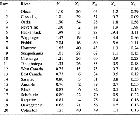
In a 1976 study exploring the relationship between water quality and land use, Haith (1976) obtained the measurements (shown in Table 1.8) on 20 river basins in New York State. A question of interest here is how the land use around a river basin contributes to the water pollution as measured by the mean nitrogen concentration (mg/liter). The data are shown in Table 1.9 and can also be found in the book's Web site.

Table 1.5 Variables for the Study of Domestic Immigration

Variable	Definition
State	State name
NDIR	Net domestic immigration rate over the period 1990–1994
Unemp	Unemployment rate in the civilian labor force in 1994
Wage	Average hourly earnings of production workers in manufacturing in 1994
Crime	Violent crime rate per 100,000 people in 1993
Income	Median household income in 1994
Metrop	Percentage of state population living in metropolitan areas in 1992
Poor	Percentage of population who fall below the poverty level in 1994
Taxes	Total state and local taxes per capita in 1993
Educ	Percentage of population 25 years or older who have a high school degree or higher in 1990
BusFail	The number of business failures divided by the population of the state in 1993
Temp	Average of the 12 monthly average temperatures (in degrees Fahrenheit) for the state in 1993
Region	Region in which the state is located (northeast, south, midwest, west)

1.4 STEPS IN REGRESSION ANALYSIS

Regression analysis includes the following steps:

• Statement of the problem
• Selection of potentially relevant variables
• Data collection
• Model specification
• Choice of fitting method
• Model fitting
• Model validation and criticism
• Using the chosen model(s) for the solution of the posed problem.

These steps are examined below.

Table 1.6 First Six Variables of the Domestic Immigration Data

Table 1.7 Last Six Variables of the Domestic Immigration Data

Table 1.8 Variables for Study of Water Pollution in New York Rivers

Variable	Definition
y	Mean nitrogen concentration (mg/liter) based on samples taken at regular intervals during the spring, summer, and fall months
X1	Agriculture: percentage of land area currently in agricultural use
X2	Forest: percentage of forest land
X3	Residential: percentage of land area in residential use
X4	Commercial/Industrial: percentage of land area in either commercial or industrial use

Table 1.9 The New York Rivers Data

1.4.1 Statement of the Problem

Regression analysis usually starts with a formulation of the problem. This includes the determination of the question(s) to be addressed by the analysis. The problem statement is the first and perhaps the most important step in regression analysis. It is important because an ill-defined problem or a misformulated question can lead to wasted effort. It can lead to the selection of irrelevant set of variables or to a wrong choice of the statistical method of analysis. A question that is not carefully formulated can also lead to the wrong choice of a model. Suppose we wish to determine whether or not an employer is discriminating against a given group of employees, say women. Data on salary, qualifications, and sex are available from the company's record to address the issue of discrimination. There are several definitions of employment discrimination in the literature. For example, discrimination occurs when on the average (a) women are paid less than equally qualified men, or (b) women are more qualified than equally paid men. To answer the question: “On the average, are women paid less than equally qualified men?” we choose salary as a response variable, and qualification and sex as predictor variables. But to answer the question: “On the average, are women more qualified than equally paid men?” we choose qualification as a response variable and salary and sex as predictor variables, that is, the roles of variables have been switched.

1.4.2 Selection of Potentially Relevant Variables

The next step after the statement of the problem is to select a set of variables that are thought by the experts in the area of study to explain or predict the response variable. The response variable is denoted by Y and the explanatory or predictor variables are denoted by X₁, X₂,…, X_p, where p denotes the number of predictor variables. An example of a response variable is the price of a single family house in a given geographical area. A possible relevant set of predictor variables in this case is: area of the lot, area of the house, age of the house, number of bedrooms, number of bathrooms, type of neighborhood, style of the house, amount of real estate taxes, etc.

1.4.3 Data Collection

The next step after the selection of potentially relevant variables is to collect the data from the environment under study to be used in the analysis. Sometimes the data are collected in a controlled setting so that factors that are not of primary interest can be held constant. More often the data are collected under nonexperimental conditions where very little can be controlled by the investigator. In either case, the collected data consist of observations on n subjects. Each of these n observations consists of measurements for each of the potentially relevant variables. The data are usually recorded as in Table 1.10. A column in Table 1.10 represents a variable, whereas a row represents an observation, which is a set of p + 1 values for a single subject (e.g., a house); one value for the response variable and one value for each of the p predictors. The notation x_ij refers to the ith value of the jth variable. The first subscript refers to observation number and the second refers to variable number.

Table 1.10 Notation for the Data Used in Regression Analysis

Each of the variables in Table 1.10 can be classified as either quantitative or qualitative. Examples of quantitative variables are the house price, number of bedrooms, age, and taxes. Examples of qualitative variables are neighborhood type (e.g., good or bad neighborhood) and house style (e.g., ranch, colonial, etc.). In this book we deal mainly with the cases where the response variable is quantitative. A technique used in cases where the response variable is binary⁶ is called logistic regression. This is introduced in Chapter 12. In regression analysis, the predictor variables can be either quantitative and/or qualitative. For the purpose of computations, however, the qualitative variables, if any, have to be coded into a set of indicator or dummy variables as discussed in Chapter 5.

If all predictor variables are qualitative, the techniques used in the analysis of the data are called the analysis of variance techniques. Although the analysis of variance techniques can be introduced and explained as methods in their own right⁷, it is shown in Chapter 5 that they are special cases of regression analysis. If some of the predictor variables are quantitative while others are qualitative, regression analysis in these cases is called the analysis of covariance.

1.4.4 Model Specification

The form of the model that is thought to relate the response variable to the set of predictor variables can be specified initially by the experts in the area of study based on their knowledge or their objective and/or subjective judgments. The hypothesized model can then be either confirmed or refuted by the analysis of the collected data. Note that the model need to be specified only in form, but it can still depend on unknown parameters. We need to select the form of the function f(X₁, X₂,…, X_p) in (1.1). This function can be classified into two types: linear and nonlinear. An example of a linear function is

while a nonlinear function is

Note that the term linear (nonlinear) here does not describe the relationship between Y and X₁, X₂,…, X_p. It is related to the fact that the regression parameters enter the equation linearly (nonlinearly). Each of the following models are linear

because in each case the parameters enter linearly although the relationship between Y and X is nonlinear. This can be seen if the two models are re-expressed, respectively, as follows:

where in the first equation we have X₁ = X and X₂ = X² and in the second equation we have X₁ = ln X. The variables here are re-expressed or transformed. Transformation is dealt with in Chapter 6. All nonlinear functions that can be transformed into linear functions are called linearizable functions. Accordingly, the class of linear models is actually wider than it might appear at first sight because it includes all linearizable functions. Note, however, that not all nonlinear functions are linearizable. For example, it is not possible to linearize the nonlinear function in (1.4). Some authors refer to nonlinear functions that are not linearizable as intrinsically nonlinear functions.

A regression equation containing only one predictor variable is called a simple regression equation. An equation containing more than one predictor variable is called a multiple regression equation. An example of simple regression would be an analysis in which the time to repair a machine is studied in relation to the number of components to be repaired. Here we have one response variable (time to repair the machine) and one predictor variable (number of components to be repaired). An example of a very complex multiple regression situation would be an attempt to explain the age-adjusted mortality rates prevailing in different geographic regions (response variable) by a large number of environmental and socioeconomic factors (predictor variables). Both types of problems are treated in this book. These two particular examples are studied, one in Chapter 2, the other in Chapter 11.

In certain applications the response variable can actually be a set of variables, Y₁, Y₂,…, Y_q, say, which are thought to be related to the same set of predictor variables, X₁, X₂,…, X_p. For example, Bartlett, Stewart, and Abrahamowicz (1998) present a data set on 148 healthy people. Eleven variables are measured; six variables represent different types of measured sensory thresholds (e.g., vibration, hand and foot temperatures) and five a priori selected baseline covariates (e.g., age, sex, height, and weight) that may have systematic effects on some or all of the six sensory thresholds. Here we have six response variables and five predictor variables. This data set, which we refer to as the QST (quantitative sensory testing) data, is not listed here due to its size (148 observations) but it can be found in the book's Web site. For further description of the data and objectives of the study, see Bartlett, Stewart, and Abrahamowicz (1998).

When we deal only with one response variable, regression analysis is called univariate regression and in cases where we have two or more response variables, the regression is called multivariate regression. Simple and multiple regressions should not be confused with univariate versus multivariate regressions. The distinction between simple and multiple regressions is determined by the number of predictor variables (simple means one predictor variable and multiple means two or more predictor variables), whereas the distinction between univariate and multivariate regressions is determined by the number of response variables (univariate means one response variable and multivariate means two or more response variables). In this book we consider only univariate regression (both simple and multiple, linear and nonlinear). Multivariate regression is treated in books on multivariate analysis such as Rencher (1995), Johnson and Wichern (1992), and Johnson (1998). In this book the term regression will be used to mean univariate regression.

The various classifications of regression analysis we discussed above are shown in Table 1.11.

1.4.5 Method of Fitting

After the model has been defined and the data have been collected, the next task is to estimate the parameters of the model based on the collected data. This is also referred to as parameter estimation or model fitting. The most commonly used method of estimation is called the least squares method. Under certain assumptions (to be discussed in detail in this book), least squares method produce estimators with desirable properties. In this book we will deal mainly with least squares method and its variants (e.g., weighted least squares). In some instances (e.g., when one or more of the assumptions does not hold) other estimation methods may be superior to least squares. The other estimation methods that we consider in this book are the maximum likelihood method, the ridge method, and the principal components method.

1.4.6 Model Fitting

The next step in the analysis is to estimate the regression parameters or to fit the model to the collected data using the chosen estimation method (e.g., least squares). The estimates of the regression parameters β₀, β₁,…, β_p in (1.1) are denoted by . The estimated regression equation then becomes

Table 1.11 Various Classifications of Regression Analysis

Type of Regression	Conditions
Univariate	Only one quantitative response variable
Multivariate	Two or more quantitative response variables
Simple	Only one predictor variable
Multiple	Two or more predictor variables
Linear	All parameters enter the equation linearly, possibly after transformation of the data
Nonlinear	The relationship between the response and some of the predictors is nonlinear or some of the parameters appear nonlinearly, but no transformation is possible to make the parameters appear linearly
Analysis of Variance	All predictors are qualitative variables
Analysis of Covariance	Some predictors are quantitative variables and others are qualitative variables
Logistic	The response variable is qualitative

A hat on top of a parameter denotes an estimate of the parameter. The value (pronounced as Y-hat) is called the fitted value. Using (1.5), we can compute n fitted values, one for each of the n observations in our data. For example, the ith fitted value _i is

where x_i1,…, x_ip are the values of the p predictor variables for the ith observation.

Note that (1.5) can be used to predict the response variable for any values of the predictor variables not observed in our data. In this case, the obtained is called the predicted value. The difference between fitted and predicted values is that the fitted value refers to the case where the values used for the predictor variables correspond to one of the n observations in our data, but the predicted values are obtained for any set of values of the predictor variables. It is generally not recommended to predict the response variable for a set of values of the predictor variables far outside the range of our data. In cases where the values of the predictor variables represent future values of the predictors, the predicted value is referred to as the forecasted value.

Figure 1.1 A schematic illustration of the iterative nature of the regression process.

1.4.7 Model Criticism and Selection

The validity of a statistical method, such as regression analysis, depends on certain assumptions. Assumptions are usually made about the data and the model. The accuracy of the analysis and the conclusions derived from an analysis depends crucially on the validity of these assumptions. Before using (1.5) for any purpose, we first need to determine whether the specified assumptions hold. We need to address the following questions:

1. What are the required assumptions?
2. For each of these assumptions, how do we determine whether or not the assumption is valid?
3. What can be done in cases where one or more of the assumptions does not hold?

The standard regression assumptions will be specified and the above questions will be addressed in great detail in various parts of this book. We emphasize here that validation of the assumptions must be made before any conclusions are drawn from the analysis. Regression analysis is viewed here as a iterative process, a process in which the outputs are used to diagnose, validate, criticize, and possibly modify the inputs. The process has to be repeated until a satisfactory output has been obtained. A satisfactory output is an estimated model that satisfies the assumptions and fits the data reasonably well. This iterative process is illustrated schematically in Figure 1.1.

1.4.8 Objectives of Regression Analysis

The explicit determination of the regression equation is the most important product of the analysis. It is a summary of the relationship between Y (the response variable) and the set of predictor variables X₁, X₂,…, X_p. The equation may be used for several purposes. It may be used to evaluate the importance of individual predictors, to analyze the effects of policy that involves changing values of the predictor variables, or to forecast values of the response variable for a given set of predictors. Although the regression equation is the final product, there are many important by-products. We view regression analysis as a set of data analytic techniques that are used to help understand the interrelationships among variables in a certain environment. The task of regression analysis is to learn as much as possible about the environment reflected by the data. We emphasize that what is uncovered along the way to the formulation of the equation may often be as valuable and informative as the final equation.

1.5 SCOPE AND ORGANIZATION OF THE BOOK

This book can be used by all who analyze data. A knowledge of matrix algebra is not necessary. We have seen excellent regression analysis done by people who have no knowledge of matrix theory. A knowledge of matrix algebra is certainly very helpful in understanding the theory. We have provided appendices which use matrix algebra for readers who are familiar with that topic. Matrix algebra permits expression of regression results much more compactly and is essential for the mathematical derivation of the results.

Lack of knowledge of matrix algebra should not deter anyone from using this book and doing regression analysis. For readers who are not familiar with matrix algebra but who wish to benefit from the material in the appendices, we recommend reading the relatively short book by Hadi (1996), Matrix Algebra As a Tool. We believe that the majority, if not all, of our readers can read it entirely on their own or with minimal assistance.

There are no formal derivations in the text and readers interested in mathematical derivations are referred to a number of books that contain formal derivations of the regression formulas. Formulas are presented, but only for purposes of reference. It is assumed throughout the book that the necessary summary statistics will be computer generated from an existing regression package.⁸

The book is organized as follows: It begins with the simple linear regression model in Chapter 2. The simple regression model is then extended to the multiple regression model in Chapter 3. In both chapters, the model is formulated, assumptions are specified, and the key theoretical results are stated and illustrated by examples. For simplicity of presentation and for pedagogical reasons, the analysis and conclusions in Chapters 2 and 3 are made under the presumption that the standard regression assumptions are valid. Chapter 4 addresses the issue of assumptions validation and the detection and correction of model violations.

Each of the remaining chapters deals with a special regression problem. Chapter 5 deals with the case where some or all of the predictor variables are qualitative. Chapter 6 deals with data transformation. Chapter 7 presents situations where a variant of the least squares method is needed. This method is called the weighted least squares method. Chapter 8 discusses the problem that arises when the observations are correlated. This problem is known as the autocorrelation problem. Chapters 9 and 10 present methods for the detection and correction of an important problem called collinearity. Collinearity occurs when the predictor variables are highly correlated.

Chapter 11 presents variable selection methods – computer methods for selecting the best and most parsimonious model(s). Before applying any of the variable selection methods, we assume in this chapter that questions of assumptions validation and model violations have already been addressed and settled satisfactorily.

The earlier chapters dealt with the case where the response variable is quantitative. Chapter 12 discusses logistic regression, the method used when the response variable is categorical. Logistic regression is studied because it is an important tool with many applications. Beside binary logistic regression, we have now included a discussion of multinomial logistic regression. This extends the application of logistic regression to more diverse situations. The categories in some multinomial are ordered, for example in attitude surveys. We also discuss the application of the logistic model to ordered response variable.

The book concludes with Chapter 13 entitled Further Topics. Two topics are discussed in this chapter. One extends the concept of linear models so that regression and logistic models are all viewed as special cases of the linear model. This extends the range of applications of linear models to more diverse situations. We also discuss Poisson regression, often used to model count data. A brief discussion of robust regression with illustrative examples is also given in this chapter.

We recommend that the chapters be covered in the same sequence as they are presented, although Chapters 5 to 12 can be covered in any order after Chapter 4, as long as Chapter 9 is covered before Chapter 10, and Chapter 7 is covered before Chapters 12 and 13.

EXERCISES

1.1 Classify each of the following variables as either quantitative or qualitative. If a variable is qualitative, state the possible categories.

(a) Geographical region	(b) Number of children in a family
(c) Price of a house	(d) Race
(e) Temperature	(t) Fuel consumption
(g) Employment rate	(h) Political party preference

1.2 Give two examples in any area of interest to you (other than those presented in Chapter 1) where regression analysis can be used as a data analytic tool to answer some questions of interest. For each example:

(a) What is the question of interest?

(b) Identify the response and the predictor variables.

(c) Classify each of the variables as either quantitative or qualitative.

(d) Which type of regression (see Table 1.11) can be used to analyze the data?

(e) Give a possible form of the model and identify its parameters.

1.3 In each of the following sets of variables, identify which of the variables can be regarded as a response variable and which can be used as predictors? (Explain)

(a) Number of cylinders and gasoline consumption of cars.

(b) SAT scores, grade point average, and college admission.

(c) Supply and demand of certain goods.

(d) Company's assets, return on a stock, and net sales.

(e) The distance of a race, the time to run the race, and the weather conditions at the time of running.

(f) The weight of a person, whether or not the person is a smoker, and whether or not the person has a lung cancer.

(g) The height and weight of a child, his/her parents' height and weight, and the sex and age of the child.

1.4 For each of the sets of variables in Exercise 1.3:

(a) Classify each variable as either quantitative or qualitative.

(b) Which type of regression (see Table 1.11) can be used in the analysis of the data?