CHAPTER 11

VARIABLE SELECTION PROCEDURES

11.1 INTRODUCTION

In our discussion of regression problems so far we have assumed that the variables that go into the equation were chosen in advance. Our analysis involved examining the equation to see whether the functional specification was correct, and whether the assumptions about the error term were valid. The analysis presupposed that the set of variables to be included in the equation had already been decided. In many applications of regression analysis, however, the set of variables to be included in the regression model is not predetermined, and it is often the first part of the analysis to select these variables. There are some occasions when theoretical or other considerations determine the variables to be included in the equation. In those situations the problem of variable selection does not arise. But in situations where there is no clear-cut theory, the problem of selecting variables for a regression equation becomes an important one.

The problems of variable selection and the functional specification of the equation are linked to each other. The questions to be answered while formulating a regression model are: Which variables should be included, and in what form should they be included; that is, should they enter the equation as an original variable X, or as some transformed variable such as X², log X, or a combination of both? Although ideally the two problems should be solved simultaneously, we shall for simplicity propose that they be treated sequentially. We first determine the variables that will be included in the equation, and after that investigate the exact form in which the variables enter it. This approach is a simplification, but it makes the problem of variable selection more tractable. Once the variables that are to be included in the equation have been selected, we can apply the methods described in the earlier chapters to arrive at the actual form of the equation.

11.2 FORMULATION OF THE PROBLEM

We have a response variable Y and q predictor variables X₁, X₂,…, X_q. A linear model that represents Y in terms of q variables is

where β_j are parameters and ε_i represents random disturbances. Instead of dealing with the full set of variables (particularly when q is large), we might delete a number of variables and construct an equation with a subset of variables. This chapter is concerned with determining which variables are to be retained in the equation. Let us denote the set of variables retained by and those deleted by . Let us examine the effect of variable deletion under two general conditions:

1. The model that connects Y to the X's has all β's nonzero.
2. The model has nonzero, but zero.

Suppose that instead of fitting (11.1) we fit the subset model

We shall describe the effect of fitting the model to the full and partial set of X's under the two alternative situations described previously. In short, what are the effects of including variables in an equation when they should be properly left out (because the population regression coefficients are zero) and the effect of leaving out variables when they should be included (because the population regression coefficients are not zero)? We will examine the effect of deletion of variables on the estimates of parameters and the predicted values of Y. The solution to the problem of variable selection becomes a little clearer once the effects of retaining unessential variables or the deletion of essential variables in an equation are known.

11.3 CONSEQUENCES OF VARIABLES DELETION

Denote the estimates of the regression parameters by when the model (11.1) is fitted to the full set of variables X₁, X₂,…, X_q. Denote the estimates of the regression parameters by when the model (11.2) is fitted. Let and be the predicted values from the full and partial set of variables corresponding to an observation . The results can now be summarized as follows (a summary using matrix notation is given in the Appendix to this chapter): are biased estimates of unless the remaining β's in the model () are zero or the variables are orthogonal to the variable set . The estimates have less precision than that is,

The variance of the estimates of regression coefficients for variables in the reduced equation are not greater than the variances of the corresponding estimates for the full model. Deletion of variables decreases or, more correctly, never increases, the variances of estimates of the retained regression coefficients. Since are biased and are not, a better comparison of the precision of estimates would be obtained by comparing the mean square errors of with the variances of . The mean squared errors (MSE) of will be smaller than the variances of , only if the deleted variables have regression coefficients smaller in magnitude than the standard deviations of the estimates of the corresponding coefficients. The estimate of σ², based on the subset model, is generally biased upward.

Let us now look at the effect of deletion of variables on prediction. The prediction is biased unless the deleted variables have zero regression coefficients, or the set of retained variables are orthogonal to the set of deleted variables. The variance of a predicted value from the subset model is smaller than or equal to the variance of the predicted value from the full model; that is,

The conditions for MSE() to be smaller than Var() are identical to the conditions for MSE() to be smaller than Var(), which we have already stated. For further details, refer to Chatterjee and Hadi (1988).

The rationale for variable selection can be outlined as follows: Even though the variables deleted have nonzero regression coefficients, the regression coefficients of the retained variables may be estimated with smaller variance from the subset model than from the full model. The same result also holds for the variance of a predicted response. The price paid for deleting variables is in the introduction of bias in the estimates. However, there are conditions (as we have described above), when the MSE of the biased estimates will be smaller than the variance of their unbiased estimates; that is, the gain in precision is not offset by the square of the bias. On the other hand, if some of the retained variables are extraneous or unessential, that is, have zero coefficients or coefficients whose magnitudes are smaller than the standard deviation of the estimates, the inclusion of these variables in the equation leads to a loss of precision in estimation and prediction.

The reader is referred to Sections 3.5, 4.12, and 4.13 for further elaboration on the interpretation of regression coefficients and the role of variables in regression modeling.

11.4 USES OF REGRESSION EQUATIONS

A regression equation has many uses. These are broadly summarized below.

11.4.1 Description and Model Building

A regression equation may be used to describe a given process or as a model for a complex interacting system. The purpose of the equation may be purely descriptive, to clarify the nature of this complex interaction. For this use there are two conflicting requirements: (1) to account for as much of the variation as possible, which points in the direction for inclusion of a large number of variables; and (2) to adhere to the principle of parsimony, which suggests that we try, for ease of understanding and interpretation, to describe the process with as few variables as possible. In situations where description is the prime goal, we try to choose the smallest number of predictor variables that accounts for the most substantial part of the variation in the response variable.

11.4.2 Estimation and Prediction

A regression equation is sometimes constructed for prediction. From the regression equation we want to predict the value of a future observation or estimate the mean response corresponding to a given observation. When a regression equation is used for this purpose, the variables are selected with an eye toward minimizing the MSE of prediction.

11.4.3 Control

A regression equation may be used as a tool for control. The purpose for constructing the equation may be to determine the magnitude by which the value of a predictor variable must be altered to obtain a specified value of the response (target) variable. Here the regression equation is viewed as a response function, with Y as the response variable. For control purposes it is desired that the coefficients of the variables in the equation be measured accurately; that is, the standard errors of the regression coefficients are small.

These are the broad uses of a regression equation. Occasionally, these functions overlap and an equation is constructed for some or all of these purposes. The main point to be noted is that the purpose for which the regression equation is constructed determines the criterion that is to be optimized in its formulation. It follows that a subset of variables that may be best for one purpose may not be best for another. The concept of the “best” subset of variables to be included in an equation always requires additional qualification.

Before discussing actual selection procedures we make two preliminary remarks. First, it is not usually meaningful to speak of the “best set” of variables to be included in a multiple regression equation. There is no unique “best set” of variables. A regression equation can be used for several purposes. The set of variables that may be best for one purpose may not be best for another. The purpose for which a regression equation is constructed should be kept in mind in the variable selection process. We shall show later that the purpose for which an equation is constructed determines the criteria for selecting and evaluating the contributions of different variables.

Second, since there is no best set of variables, there may be several subsets that are adequate and could be used in forming an equation. A good variable selection procedure should point out these several sets rather than generate a so-called single “best” set. The various sets of adequate variables throw light on the structure of data and help us in understanding the underlying process. In fact, the process of variable selection should be viewed as an intensive analysis of the correlational structure of the predictor variables and how they individually and jointly affect the response variable under study. These two points influence the methodology that we present in connection with variable selection.

11.5 CRITERIA FOR EVALUATING EQUATIONS

To judge the adequacy of various fitted equations we need a criterion. Several have been proposed in the statistical literature. We describe the two that we consider most useful. An exhaustive list of criteria is found in Hocking (1976).

11.5.1 Residual Mean Square

One measure that is used to judge the adequacy of a fitted equation is the residual mean square (RMS). With a p-term equation (includes a constant and (p − 1) variables), the RMS is defined as

where SSE_p is the residual sum of squares for a p-term equation. Between two equations, the one with the smaller RMS is usually preferred, especially if the objective is forecasting.

It is clear that RMS_p is related to the square of the multiple correlation coefficient and the square of the adjusted multiple correlation coefficient which have already been described (Chapter 3) as measures for judging the adequacy of fit of an equation. Here we have added a subscript to R² and to denote their dependence on the number of terms in an equation. The relationship between these quantities are given by

and

where

Note that is more appropriate than when comparing models with different number of predictors because adjusts (penalizes) for the number of predictor variables in the model.

11.5.2 Mallows C_p

We pointed out earlier that predicted values obtained from a regression equation based on a subset of variables are generally biased. To judge the performance of an equation we should consider the mean square error of the predicted value rather than the variance. The standardized total mean squared error of prediction for the observed data is measured by

where MSE() is the mean squared error of the ith predicted value from a p-term equation, and σ² is the variance of the random errors. The MSE() has two components, the variance of prediction arising from estimation, and a bias component arising from the deletion of variables.

To estimate J_p, Mallows (1973) uses the statistic

where is an estimate of σ² and is usually obtained from the linear model with the full set of q variables. It can be shown that the expected value of C_p is p when there is no bias in the fitted equation containing p terms. Consequently, the deviation of C_p from p can be used as a measure of bias. The C_p statistic therefore measures the performance of the variables in terms of the standardized total mean square error of prediction for the observed data points irrespective of the unknown true model. It takes into account both the bias and the variance. Subsets of variables that produce values of C_p that are close to p are the desirable subsets. The selection of “good” subsets is done graphically. For the various subsets a graph of C_p is plotted against p. The line C_p = p is also drawn on the graph. Sets of variables corresponding to points close to the line C_p = p are the good or desirable subsets of variables to form an equation. The use of C_p plots is illustrated and discussed in more detail in the example that is given in Section 11.10. A very thorough treatment of the C_p statistic is given in Daniel and Wood (1980).

11.5.3 Information Criteria: Akaike and Other Modified Forms

Variable selection in the regression context can be viewed as a model selection problem. The Information criteria that we now describe arose first in the general problem of model selection. The Akaike (1973) Information Criteria (AIC) in selecting a model tries to balance the conflicting demands of accuracy (fit) and simplicity (small number of variables). This is the principle of parsimony already discussed in Section 3.9.2. AIC for a p-term equation (a constant, and (p − 1) variables) is given by

The models with smaller AIC are preferred.

We can see from (11.8) that for two models with similar SSE, AIC penalizes the model that has larger number of variables. The numerical value of AIC for a single model is not very meaningful or descriptive. AIC can be used, however, to rank the models on the basis of their twin criteria of fit and simplicity. Models with AIC not differing by 2 should be treated as equally adequate. Larger differences in AIC indicate significant difference between the quality of the models. The one with the lower AIC should be adopted.

A great advantage of AIC is that it allows us to compare non-nested models. A group of models are nested if they can be obtained from a larger model as special cases (See Section 3.9). We cannot perform an F-test, for example, to compare the adequacy of a model based on (X₁, X₂, X₃) with one based on (X₄, X₅). The choice of these two sets of variables may be dictated by the nature of the problem at hand. The AIC will allow us to make such comparisons but not the F-test described earlier.

To compare models by AIC we must have a complete data cases (no missing values). The AIC must be calculated on the same set of observations. If there are many missing values for some variables, application of AIC may be inefficient because observations in which some variables were missing will be dropped.

Several modifications of AIC have been suggested. One popular variation called Bayes Information Criteria (BIC), originally proposed by Schwarz (1978), is defined as

The difference between AIC and BIC is in the severity of penalty for p. The penalty is far more severe in BIC when n > 8. This tends to control the overfitting (resulting in a choice of larger p) tendency of AIC.

Another modification of AIC to avoid overfitting is the bias corrected version, AIC^c, proposed by Hurvich and Tsai (1989), is given by

The correction to AIC in (11.10) is small for large n and moderate p. The correction is large when n is small and p large. One should never fit a large and complex model with a small number of observations. In general the correction to AIC will be minor, and we will not discuss AIC^c further. To guard against overfitting in our analysis we will examine BIC.

11.6 MULTICOLLINEARITY AND VARIABLE SELECTION

In discussing variable selection procedures, we distinguish between two broad situations:

1. The predictor variables are not collinear; that is, there is no strong evidence of multicollinearity.
2. The predictor variables are collinear; that is, the data are highly multicollinear.

Depending on the correlation structure of the predictor variables, we propose different approaches to the variable selection procedure. If the data analyzed are not collinear, we proceed in one manner, and if collinear, we proceed in another.

As a first step in variable selection procedure we recommend calculating the variance inflation factors (VIFs) or the eigenvalues of the correlation matrix of the predictor variables. If none of the VIFs are greater than 10, collinearity is not a problem. Further, as we explained in Chapter 9, the presence of small eigenvalues indicates collinearity. If the condition number¹ is larger than 15, the variables are collinear. We may also look at the sum of the reciprocals of the eigenvalues. If any of the individual eigenvalues are less than 0.01, or the sum of the reciprocals of the eigenvalues is greater than, say, five times the number of predictor variables in the problem, we say that the variables are collinear. If the conditions above do not hold, the variables are regarded as noncollinear.

11.7 EVALUATING ALL POSSIBLE EQUATIONS

The first procedure described is very direct and applies equally well to both collinear and noncollinear data. The procedure involves fitting all possible subset equations to a given body of data. With q variables the total number of equations fitted is 2^q (including an equation that contains all the variables and another that contains no variables). The latter is simply , which is obtained from fitting the model Y = β₀ + ε. This method clearly gives an analyst the maximum amount of information available concerning the nature of relationships between Y and the set of X's. However, the number of equations and supplementary information that must be looked at may be prohibitively large. Even with only six predictor variables, there are 64 (2⁶) equations to consider; with seven variables the number grows to 128 (2⁷), neither feasible nor practical. An efficient way of using the results from fitting all possible equations is to pick out the three “best” (on the basis of R², C_p, RMS, or the information criteria outlined earlier) equations containing a specified number of variables. This smaller subset of equations is then analyzed to arrive at the final model. These regressions are then carefully analyzed by examining the residuals for outliers, autocorrelation, or the need for transformations before deciding on the final model. The various subsets that are investigated may suggest interpretations of the data that might have been overlooked in a more restricted variable selection approach.

When the number of variables is large, the evaluation of all possible equations may not be practically feasible. Certain shortcuts have been suggested (Fumival and Wilson, 1974; La Motte and Hocking, 1970) which do not involve computing the entire set of equations while searching for the desirable subsets. But with a large number of variables these methods still involve a considerable amount of computation. There are variable selection procedures that do not require the evaluation of all possible equations. Employing these procedures will not provide the analyst with as much information as the fitting of all possible equations, but it will entail considerably less computation and may be the only available practical solution. These are discussed in Section 11.8. These procedures are quite efficient with noncollinear data. We do not, however, recommend them for collinear data.

11.8 VARIABLE SELECTION PROCEDURES

For cases when there are a large number of potential predictor variables, a set of procedures that does not involve computing of all possible equations has been proposed. These procedures have the feature that the variables are introduced or deleted from the equation one at a time, and involve examining only a subset of all possible equations. With q variables these procedures will involve evaluation of at most (q + 1) equations, as contrasted with the evaluation of 2^q equations necessary for examining all possible equations. The procedures can be classified into two broad categories: (1) the forward selection procedure (FS), and (2) the backward elimination procedure (BE). There is also a very popular modification of the FS procedure called the stepwise method. The three procedures are described and compared below.

11.8.1 Forward Selection Procedure

The forward selection procedure starts with an equation containing no predictor variables, only a constant term. The first variable included in the equation is the one which has the highest simple correlation with the response variable Y. If the regression coefficient of this variable is significantly different from zero it is retained in the equation, and a search for a second variable is made. The variable that enters the equation as the second variable is one which has the highest correlation with Y, after Y has been adjusted for the effect of the first variable, that is, the variable with the highest simple correlation coefficient with the residuals from Step 1. The significance of the regression coefficient of the second variable is then tested. If the regression coefficient is significant, a search for a third variable is made in the same way. The procedure is terminated when the last variable entering the equation has an insignificant regression coefficient or all the variables are included in the equation. The significance of the regression coefficient of the last variable introduced in the equation is judged by the standard t-test computed from the latest equation. Most forward selection algorithms use a low t cutoff value for testing the coefficient of the newly entered variable; consequently, the forward selection procedure goes through the full set of variables and provides us with q + 1 possible equations.

11.8.2 Backward Elimination Procedure

The backward elimination procedure starts with the full equation and successively drops one variable at a time. The variables are dropped on the basis of their contribution to the reduction of error sum of squares. The first variable deleted is the one with the smallest contribution to the reduction of error sum of squares. This is equivalent to deleting the variable which has the smallest t-test in the equation. If all the t-tests are significant, the full set of variables is retained in the equation. Assuming that there are one or more variables that have insignificant t-tests, the procedure operates by dropping the variable with the smallest insignificant t-test. The equation with the remaining (q − 1) variables is then fitted and the t-tests for the new regression coefficients are examined. The procedure is terminated when all the t-tests are significant or all variables have been deleted. In most backward elimination algorithms the cutoff value for the t-test is set high so that the procedure runs through the whole set of variables, that is, starting with the q-variable equation and ending up with an equation containing only the constant term. The backward elimination procedure involves fitting at most q + 1 regression equations

11.8.3 Stepwise Method

The stepwise method is essentially a forward selection procedure but with the added proviso that at each stage the possibility of deleting a variable, as in backward elimination, is considered. In this procedure a variable that entered in the earlier stages of selection may be eliminated at later stages. The calculations made for inclusion and deletion of variables are the same as FS and BE procedures. Often, different levels of significance are assumed for inclusion and exclusion of variables from the equation.

AIC and BIC both can be used for setting up stepwise procedures (forward selection and backward elimination). For forward selection one starts with a constant as the fitting term, and adds variables to the model. The procedure is terminated, when addition of a variable causes no reduction of AIC (BIC). In the backward procedure, we start with the full model (containing all the variables) and drop variables successively. The procedure is terminated when dropping a variable does not lead to any further reduction in the criteria.

The stepwise procedure based on information criteria differs in a major way from the procedures based on the t-statistic that gauges the significance of a variable. The information based procedures are driven by all the variables in the model. The termination of the procedure is based solely on the decrease of the criterion, and not on the statistical significance of the entering or departing variable.

Most of the currently available software do not automatically produce AIC or BIC. They all, however, provide SSE, from which it is easy to compute (11.8) and (11.9) the information criteria.

11.9 GENERAL REMARKS ON VARIABLE SELECTION METHODS

The variable selection procedures discussed above should be used with caution. These procedures should not be used mechanically to determine the “best” variables. The order in which the variables enter or leave the equation in variable selection procedures should not be interpreted as reflecting the relative importance of the variables. If these caveats are kept in mind, the variable selection procedures are useful tools for variable selection in noncollinear situations. All three procedures will give nearly the same selection of variables with noncollinear data. They entail much less computing than that in the analysis of all possible equations.

Several stopping rules have been proposed for the variable selection procedures. A stopping rule that has been reported to be quite effective is as follows:

• In FS: Stop if minimum t-test is less than 1.
• In BE: Stop if minimum t-test is greater than 1.

In the following example we illustrate the effect of different stopping rules in variable selection.

We recommend the BE procedure over FS procedure for variable selection. One obvious reason is that in BE procedure the equation with the full variable set is calculated and available for inspection even though it may not be used as the final equation. Although we do not recommend the use of variable selection procedures in a collinear situation, the BE procedure is better able to handle multicollinearity than the FS procedure (Mantel, 1970).

In an application of variable selection procedures several equations are generated, each equation containing a different number of variables. The various equations generated can then be evaluated using a statistic such as C_p, RMS, AIC, or BIC. The residuals for the various equations should also be examined. Equations with unsatisfactory residual plots are rejected. Only a total and comprehensive analysis will provide an adequate selection of variables and a useful regression equation. This approach to variable selection is illustrated by the following example.

Table 11.1 Correlation Matrix for the Supervisor Performance Data in Table 3.3

11.10 A STUDY OF SUPERVISOR PERFORMANCE

To illustrate variable selection procedures in a noncollinear situation, consider the Supervisor Performance data discussed in Section 3.3. A regression equation was needed to study the qualities that led to the characterization of good supervisors by the people being supervised. The equation is to be constructed in an attempt to understand the supervising process and the relative importance of the different variables. In terms of the use for the regression equation, this would imply that we want accurate estimates of the regression coefficients, in contrast to an equation that is to be used only for prediction. The variables in the problem are given in Table 3.2. The data are shown in Table 3.3 and can also be obtained from the book's Web site.²

The VIFs resulting from regressing Y on X₁, X₂,…, X₆ are

The range of the VIFs (1.2 to 3.1) shows that collinearity is not a problem for these data. The same picture emerges if we examine the eigenvalues of the correlation matrix of the data (Table 11.1). The eigenvalues of the correlation matrix are:

The sum of the reciprocals of the eigenvalues is 12.8. Since none of the eigenvalues are small (the condition number is 4.1) and the sum of the reciprocals of the eigenvalues is only about twice the number of variables, we conclude that the data in the present example are not seriously collinear and we can apply the variable selection procedures just described.

The result of forward selection procedure is given in Table 11.2. For successive equations we show the variables present, the RMS, and the value of the C_p statistic. The column labeled Rank shows the rank of the subset obtained by FS relative to best subset (on the basis of RMS) of same size. The value of p is the number of predictor variables in the equation, including a constant term. Two stopping rules are used:

Table 11.2 Variables Selected by the Forward Selection Method

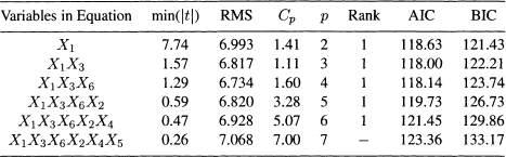
  1. Stop if minimum absolute t-test is less than t_0.05(n − p).

  2. Stop if minimum absolute t-test is less than 1.

The first rule is more stringent and terminates with variables X₁ and X₃. The second rule is less stringent and terminates with variables X₁, X₃, and X₆.

The results of applying the BE procedure are presented in Table 11.3. They are identical in structure to Table 11.2. For the BE we will use the stopping rules:

 1. Stop if minimum absolute t-test is greater than t_0.05(n − p).

 2. Stop if minimum absolute t-test is greater than 1.

With the first stopping rule the variables selected are X₁ and X₃. With the second stopping rule the variables selected are X₁, X₃, and X₆. The FS and BE give identical equations for this problem, but this is not always the case (an example is given in Section 11.12). To describe the supervisor performance, the equation

is chosen. The residual plots (not shown) for this equation are satisfactory. Since the present problem has only six variables, the total number of equations that can be fitted which contain at least one variable is 63. The C_p values for all 63 equations are shown in Table 11.4. The C_p values are plotted against p in Figure 11.1. The best subsets of variables based on C_p values are given in Table 11.5.

It is seen that the subsets selected by C_p are different from those arrived at by the variable selection procedures as well as those selected on the basis of residual mean square. This anomaly suggests an important point concerning the C_p statistic that the reader should bear in mind. For applications of the C_p statistic, an estimate of σ² is required. Usually, the estimate of σ² is obtained from the residual sum of squares from the full model. If the full model has a large number of variables with no explanatory power (i.e., population regression coefficients are zero), the estimate of σ² from the residual sum of squares for the full model would be large. The loss in degrees of freedom for the divisor would not be balanced by a reduction in the error sum of squares. If is large, then the value of C_p is small. For C_p to work properly, a good estimate of σ² must be available. When a good estimate of σ² is not available, C_p is of only limited usefulness. In our present example, the RMS for the full model with six variables is larger than the RMS for the model with three variables X₁, X₃, X₆. Consequently, the C_p values are distorted and not very useful in variable selection in the present case. The type of situation we have described can be spotted by looking at the RMS for different values of p. RMS will at first tend to decrease with p, but increase at later stages. This behavior indicates that the latter variables are not contributing significantly to the reduction of error sum of squares. Useful application of C_p requires a parallel monitoring of RMS to avoid distortions.

Table 11.3 Variables Selected by Backward Elimination Method

Table 11.4 Values of C_p Statistic (All Possible Equations)

Table 11.5 Variables Selected on the Basis of C_p Statistic

Figure 11.1 Supervisor's Performance Data: Scatter plot of C_p versus p for subsets with C_p < 10.

Values of AIC and BIC for forward selection and backward elimination is given in Tables 11.2 and 11.3. The lowest value of AIC (118.00) is obtained for X₁ and X₃. If we regard models with AIC within 2 to be equivalent, then X₁, X₁X₃, X₁X₃X₆, X₁X₃X₆X₂, should be considered. Among these four candidate models we can pick one of them. The lowest value of BIC (121.43) is attained by X₁. There is only one other model (X₁X₃) whose BIC lies within 2 units. It should be noted that BIC selects models with smaller number of variables because of its penalty function. Variable selection should not be done mechanically. In many situations there may not be a “best model” or a “best set of variables”. The aim of the analysis should be to identify all models of high equal adequacy.

11.11 VARIABLE SELECTION WITH COLLINEAR DATA

In Chapter 9 it was pointed out that serious distortions are introduced in standard analysis with collinear data. Consequently, we recommend a different set of procedures for selecting variables in these situations. Collinearity is indicated when the correlation matrix has one or more small eigenvalues. With a small number of collinear variables we can evaluate all possible equations and select an equation by methods that have already been described. But with a larger number of variables this method is not feasible.

Two different approaches to the problem have been proposed. The first approach tries to break down the collinearity of the data by deleting variables. The collinear structure present in the variables is revealed by the eigenvectors corresponding to the very small eigenvalues (see Chapters 9 and 10). Once the collinearities are identified, a set of variables can then be deleted to produce a reduced noncollinear data set. We can then apply the methods described earlier. The second approach uses ridge regression as the main tool. We assume that the reader is familiar with the basic terms and concepts of ridge regression (Chapter 10). The first approach (by judicious dropping of correlated variables) is the one that is almost always used in practice.

11.12 THE HOMICIDE DATA

In a study investigating the role of firearms in accounting for the rising homicide rate in Detroit, data were collected for the years 1961–1973. The data are reported in Gunst and Mason (1980), p. 360. The response variable (the homicide rate) and the predictor variables believed to influence or be related to the rise in the homicide rate are defined in Table 11.6 and given in Tables 11.7 and 11.8. The data can also be found in the book's Web site.

We use these data to illustrate the danger of mechanical variable selection procedures, such as the FS and BE, in collinear situations. We are interested in fitting the model

In terms of the centered and scaled version of the variables, the model becomes

The OLS results are shown in Table 11.9. Can the number of predictor variables in this model be reduced? If the standard assumptions hold, the small t-test for the variable G (0.68) would indicate that the corresponding regression coefficient is insignificant and G can be omitted from the model. Let us now apply the forward selection and the backward elimination procedures to see which variables are selected. The regression output that we need to implement the two methods on the standardized versions of the variables are summarized in Table 11.10. In this table we give the estimated coefficients, their t-tests, and the adjusted squared multiple correlation coefficient, for each model for comparison purposes.

Table 11.6 Homicide Data: Description of Variables

Table 11.7 First Part of the Homicides Data

Table 11.8 Second Part of the Homicide Data

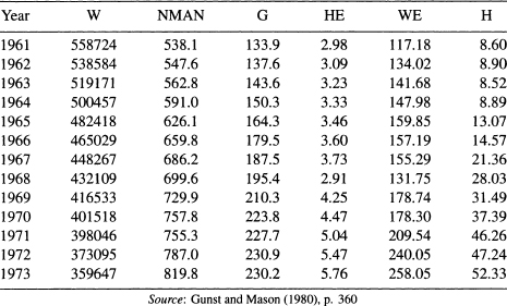
Table 11.9 Homicide Data: The OLS Results From Fitting Model (11.11)

The first variable to be selected by the FS is G because it has the largest t-test among the three models that contain a single variable (Models (a) to (c) in Table 11.10). Between the two candidates for the two-variable models (Models (d) and (e)), Model (d) is better than Model (e). Therefore, the second variable to enter the equation is M. The third variable to enter the equation is W (Model (f)) because it has a significant t-test. Note, however, the dramatic change of the significance of G in Models (a), (d), and (f). It was highly significant coefficient in Models (a) and (d), but became insignificant in Model (f). Collinearity is a suspect!

Table 11.10 Homicide Data: The Estimated Coefficients, Their t-tests, and the Adjusted Squared Multiple Correlation Coefficient,

The BE methods starts with the three-variable Model (f). The first variable to leave is G (because it has the lowest t-test), which leads to Model (g). Both M and W in Model (g) have significant t-tests and the BE procedure terminates

Observe that the first variable eliminated by the BE (G) is the same as the first variable selected by the FS. That is, the variable G, which was selected by the FS as the most important of the three variables, was regarded by the BE as the least important! Among other things, the reason for this anomalous result is collinearity. The eigenvalues of the correlation matrix, λ₁ = 2.65, λ₂ = 0.343, and λ₃ = 0.011, give a large condition number (k = 15.6). Two of the three variables (G and W) have large VIP (42 and 51). The sum of the reciprocals of the eigenvalues is also very large (96). In addition to collinearity, since the observations were taken over time (for the years 1961–1973), we are dealing with time series data here. Consequently, the error terms can be autocorrelated (see Chapter 8). Examining the pairwise scatter plots of the data will reveal other problems with the data.

This example shows clearly that automatic applications of variable selection procedure in multicollinear data can lead to the selection of a wrong model. In Sections 11.13 and 11.14 we make use of ridge regression for the process of variable selection in multicollinear situations.

11.13 VARIABLE SELECTION USING RIDGE REGRESSION

One of the goals of ridge regression is to produce a regression equation with stable coefficients. The coefficients are stable in the sense that they are not affected by slight variations in the estimation data. The objectives of a good variable selection procedure are (1) to select a set of variables that provides a clear understanding of the process under study, and (2) to formulate an equation that provides accurate forecasts of the response variable corresponding to values of the predictor variables not included in the study. It is seen that the objectives of a good variable selection procedure and ridge regression are very similar and, consequently, one (ridge regression) can be employed to accomplish the other (variable selection).

The variable selection is done by examining the ridge trace, a plot of the ridge regression coefficients against the ridge parameter k. For a collinear system, the characteristic pattern of ridge trace has been described in Chapter 10. The ridge trace is used to eliminate variables from the equation. The guidelines for elimination are:

1. Eliminate variables whose coefficients are stable but small. Since ridge regression is applied to standardized data, the magnitude of the various coefficients are directly comparable.
2. Eliminate variables with unstable coefficients that do not hold their predicting power, that is, unstable coefficients that tend to zero.
3. Eliminate one or more variables with unstable coefficients. The variables remaining from the original set, say p in number, are used to form the regression equation.

At the end of each of the above steps, we refit the model that includes the remaining variables before we proceed to the next step.

The subset of variables remaining after elimination should be examined to see if collinearity is no longer present in the subset. We illustrate this procedure by an example.

11.14 SELECTION OF VARIABLES IN AN AIR POLLUTION STUDY

McDonald and Schwing (1973) present a study that relates total mortality to climate, socioeconomic, and pollution variables. Fifteen predictor variables selected for the study are listed in Table 11.11. The response variable is the total age-adjusted mortality from all causes. We will not comment on the epidemiological aspects of the study, but merely use the data as an illustrative example for variable selection. A very detailed discussion of the problem is presented by McDonald and Schwing in their paper and we refer the interested reader to it for more information.

The original data are not available to us, but the correlation matrix of the response and the 15 predictor variables is given in Table 11.12. It is not a good practice to perform the analysis based only on the correlation matrix because without the original data we will not be able to perform diagnostics checking which is necessary in any thorough data analysis. To start the analysis we shall assume that the standard assumptions of the linear regression model hold. As can be expected from the nature of the variables, some of them are highly correlated with each other. The evidence of collinearity is clearly seen if we examine the eigenvalues of the correlation matrix. The eigenvalues are

Table 11.11 Description of Variables, Means, and Standard Deviations, SD (n = 60)

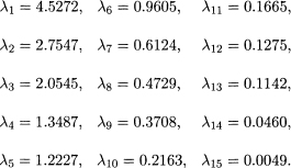
There are two very small eigenvalues; the largest eigenvalue is nearly 1000 times larger than the smallest eigenvalue. The sum of the reciprocals of the eigenvalues is 263, which is nearly 17 times the number of variables. The data show strong evidence of collinearity.

The initial OLS results from fitting a linear model to the centered and scaled data are given in Table 11.13. Although the model has a high R², some of the estimated coefficients have small t-tests. In the presence of multicollinearity, a small t-test does not necessarily mean that the corresponding variable is not important. The small t-test might be due of variance inflation because of the presence of multicollinearity. As can be seen in Table 11.13, VIF₁₂ and VIF₁₃ are very large.

Table 11.12 Correlation Matrix for the Variables in Table 11.11.

Table 11.13 OLS Regression Output for the Air Pollution Data (Fifteen Predictor Variables)

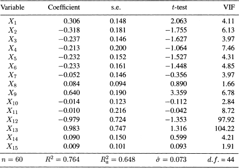
Figure 11.2 Air Pollution Data: Ridge trace S_k for θ₁,…, θ₅ (the 15-variable-model).

The ridge trace for the 15 regression coefficients are shown in Figures 11.2 to 11.4. Each Figure shows five curves. If we put all 15 curves, the graph would be quite cluttered and the curves would be difficult to trace. To make the three graphs comparable, the scale is kept the same for all graphs. From the ridge trace, we see that some of the coefficients are quite unstable and some are small regardless of the value of the ridge parameter k.

We now follow the guidelines suggested for the selection of variables in multicollinear data. Following the first criterion we eliminate variables 7, 8, 10, 11, and 15. These variables all have fairly stable coefficients, as shown by the flatness of their ridge traces, but are very small. Although variable 14 has a small coefficient at k = 0 (see Table 11.13), its value increases sharply as k increases from zero. So, it should not be eliminated at this point.

Figure 11.3 Air Pollution Data: Ridge traces for (the 15-variable-model).

Figure 11.4 Air Pollution Data: Ridge traces for (the 15-variable-model).

We now repeat the analysis using the ten remaining variables: 1, 2, 3, 4, 5, 6, 9, 12, 13, and 14. The corresponding OLS results are given in Table 11.14. There is still an evidence of multicollinearity. The largest eigenvalue, λ₁= 3.377, is about 600 times the smallest value λ₁₀ = 0.005. The two VIPs for variable 12 and 13 are still high. The corresponding ridge traces are shown in Figures 11.5 and 11.6. Variable 14 continues to have a small coefficient at k = 0 but it increases as k increases from zero. So, it should be kept in the model at this stage. None of the other nine variables satisfy the first criterion.

The second criterion suggests eliminating variables with unstable coefficients that tend to zero. Examination of the ridge traces in Figures 11.5 and 11.6 shows that variables 12 and 13 fall in this category.

The OLS results for the remaining 8 variables are shown in Table 11.15. Collinearity has disappeared. Now, the largest and smallest eigenvalues are 2.886 and 0.094, which give a small condition number (k = 5.5). The sum of the reciprocals of the eigenvalues is 23.5, about twice the number of variables. All values of VIF are less than 10. Since the retained variables are not collinear, we can now apply the variables selection methods for non-collinear data discussed in Sections 11.7 and 11.8. This is left as an exercise for the reader.

Table 11.14 OLS Regression Output for the Air Pollution Data (Ten Predictor Variables)

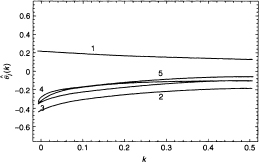
Figure 11.5 Air Pollution Data: Ridge traces for (the ten-variable-model).

An alternative way of analyzing these Air Pollution data is as follows: The collinearity in the original 15 variables is actually a simple case of multicollinearity; it involves only two variables (12 and 13). So, the analysis can proceed by eliminating anyone of the two variables. The reader can verify that the remaining 14 variables are not collinear. The standard variables selection procedures for non-collinear data can now be utilized. We leave this as an exercise for the reader.

In our analysis of the Air Pollution data, we did not use the third criterion, but there are situations where this criterion is needed. We should note that ridge regression was used successfully in this example as a tool for variable selection. Because the variables selected at an intermediate stage were found to be noncollinear, the standard OLS was utilized.

Figure 11.6 Air Pollution Data: Ridge traces for and (the ten-variable-model).

Table 11.15 OLS Regression Output for the Air Pollution Data (Eight Predictor Variables)

An analysis of these data not using ridge regression has been given by Henderson and Velleman (1981). They present a thorough analysis of the data and the reader is referred to their paper for details.

Some General Comments: We hope it is clear from our discussion that variable selection is a mixture of art and science, and should be performed with care and caution. We have outlined a set of approaches and guidelines rather than prescribing a formal procedure. In conclusion, we must emphasize the point made earlier that variable selection should not be performed mechanically as an end in itself but rather as an exploration into the structure of the data analyzed, and as in all true explorations, the explorer is guided by theory, intuition, and common sense.

11.15 A POSSIBLE STRATEGY FOR FITTING REGRESSION MODELS

In the concluding section of the chapter we outline a possible sequence of steps that may be used to fit a regression model satisfactorily. Let us emphasize at the beginning that there is no single correct approach. The reader may be more comfortable with a different sequence of steps and should feel free to follow such a sequence. In almost all cases the analysis described here will lead to meaningful interpretable models useful in real-life applications.

We assume that we have a response variable Y which we want to relate to some or all of a set of variables X₁, X₂,…, X_p. The set, X₁, X₂,…, X_p, is often generated from external subject matter considerations. The set of variables is often large and we want to come to an acceptable reduced set. Our objective is to construct a valid and viable regression model. A possible sequence of steps are:

1. Examine the variables (Y, X₁, X₂,…, X_p) one at a time. This can be done by calculating the summary statistics, and also graphically by looking at histograms, dot plots, or box plots (see Chapter 4). The distributions of the values should not be too skewed, nor the range of the variables very large. Look for outliers (check for transcription errors). Make transformations to induce symmetry and reduce skewness. Logarithmic transformations are useful in this situation (see Chapter 6).

2. Construct pairwise scatter plots for each variable. When p, the number of predictor variables, is large, this may not be feasible. Pairwise scatter plots are quite informative on the relationship between two variables. A look at the correlation matrix will point out obvious collinearity problems. Delete redundant variables. Calculate the condition number of the correlation matrix to get an idea of the severity of the collinearity (Chapters 9 and 10).

3. Fit the full linear regression model. Delete variables with no significant explanatory power (insignificant t-tests). For the reduced model, examine the residuals:

(a) Check linearity. Ifnone, make a transformation on the variable (Chapter 6).

(b) Check for heteroscedasticity and autocorrelation (for time series data). If present, take appropriate action (Chapters 7 and 8).

(c) Look for outliers, high leverage points, and influential points. If present, take appropriate action (Chapter 4).

4. Examine if additional variables can be dropped without compromising the integrity of the model. Examine if new variables are to be brought into the model (added variable plots, residual plus component plots) (Chapters 4 and 11). Repeat Step 3. Monitor the fitting process by examining the information criteria (AIC or BIC). This is particularly relevant in examining non-nested models.

5. For the final fitted model, check variance inflation factors. Ensure satisfactory residual plots and no negative diagnostic messages (Chapters 3, 5, 6, and 9). If need be, repeat Step 4.

6. Attempt should then be made to validate the fitted model. When the amount of data is large, the model may be fitted by part of the data and validated by the remainder of the data. Resampling methods such as bootstrap, jackknife, and cross-validation are also possibilities, particularly when the amount of data available is not large [see Efron (1982) and Diaconis and Efron (1983)].

The steps we have described are, in practice, often not done sequentially but implemented synchronously. The process described is an iterative process and it may be necessary to recycle through the outlined steps several times to arrive at a satisfactory model. They enumerate the factors that must be considered for constructing a satisfactory model.

One important component that we have not included in our outlined steps is the subject matter knowledge of the analyst in the area in which the model is constructed. This knowledge should always be incorporated in the model-building process. Incorporation of this knowledge will often accelerate the process of arriving at a satisfactory model because it will help considerably in the appropriate choice of variables and corresponding transformations. After all is said and done, statistical model building is an art. The techniques that we have described are the tools by which this task can be attempted methodically.

11.16 BIBLIOGRAPHIC NOTES

There is a vast amount of literature on variable selection scattered in statistical journals. A very comprehensive review with an extensive bibliography may be found in Hocking (1976). A detailed treatment on variable selection with special emphasis on C_p statistic is given in the book by Daniel and Wood (1980). Refinements on the application of C_p statistic are given by Mallows (1973). The variable selection procedures are discussed in the book by Draper and Smith (1998). Use of ridge regression in connection with variable selection is discussed by Hoerl and Kennard (1970) and by McDonald and Schwing (1973).

EXERCISES

11.1 As we have seen in Section 11.14, the three noncollinear subsets of predictor variables below have emerged. Apply one or more variable selection methods to each subset and compare the resulting final models:

(a) The subset of eight variables: 1, 2, 3, 4, 5, 6, 9, and 14.

(b) The subset of 14 variables obtained after omitting variable 12.

Table 11.16 List of Variables for Data in Table 11.17

Variable	Definition
Y	Sale price of the house in thousands of dollars
X1	Taxes (local, county, school) in thousands of dollars
X2	Number of bathrooms
X3	Lot size (in thousands of square feet)
X4	Living space (in thousands of square feet)
X5	Number of garage stalls
X6	Number of rooms
X7	Number of bedrooms
X8	Age of of the home (years)
X9	Age of of the home (years)
X9	Number of fireplaces

(c) The subset of 14 variables obtained after omitting variable 13.

11.2 The estimated regression coefficients in Table 11.13 correspond to the standardized versions of the variables because they are computed using the correlation matrix of the response and predictor variables. Using the means and standard deviations of the variables in Table 11.11, write the estimated regresion equation in terms of the original variables (before centering and scaling).

11.3 In the Homicide data discussed in Section 11.12, we observed that when fitting the model in (11.11), the FS and BE methods give contradictory results. In fact, there are several other subsets in the data (not necessarily with three predictor variables) for which the FS and BE methods give contradictory results. Find one or more of these subsets.

11.4 Use the variable selection methods, as appropriate, to find one or more subsets of the predictor variables in Tables 11.7 and 11.8 that best account for the variability in the response variable H.

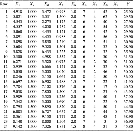
11.5 Property Valuation: Scientific mass appraisal is a technique in which linear regression methods applied to the problem of property valuation. The objective in scientific mass appraisal is to predict the sale price of a home from selected physical characteristics of the building and taxes (local, school, county) paid on the building. Twenty-four observations were obtained from Multiple Listing (Vol. 87) for Erie, PA, which is designated as Area 12 in the directory. These data (Table 11.17) were originally presented by Narula and Wellington (1977). The list of variables are given in Table 11.16.

Answer the following questions, in each case justifying your answer by appropriate analyses.

Table 11.17 Building Characteristics and Sales Price

(a) In a fitted regression model that relates the sale price to taxes and building characteristics, would you include all the variables?

(b) A veteran real estate agent has suggested that local taxes, number of rooms, and age of the house would adequately describe the sale price. Do you agree?

(c) A real estate expert who was brought into the project reasoned as follows: The selling price of a home is determined by its desirability and this is certainly a function of the physical characteristic of the building. This overall assessment is reflected in the local taxes paid by the homeowner; consequently, the best predictor of sale price is the local taxes. The building characteristics are therefore redundant in a regression equation which includes local taxes. An equation that relates sale price solely to local taxes would be adequate. Examine this assertion by examining several models. Do you agree? Present what you consider to be the most adequate model or models for predicting sale price of homes in Erie, PA.

11.6 Refer to the Gasoline Consumption data in Tables 9.18 and 9.19.

(a) Would you include all the variables to predict the gasoline consumption of the cars? Explain, giving reasons.

(b) Six alternative models have been suggested:

(a)  Regress Y on X₁.

(b)   Regress Y on X₁₀.

(c)   Regress Y on X₁ and X₁₀.

(d)   Regress Y on X₂ and X₁₀.

(e)   Regress Y on X₈ and X₁₀.

(f)   Regress Y on X₈ and X₅ and X₁₀.

Among these regression models, which would you choose to predict the gasoline consumption of automobiles? Can you suggest a better model?

(c) Plot Y against X₁, X₂, X₈, and X₁₀ (one at a time). Do the plots suggest that the relationship between Y and the 11 predictor variables may not be linear?

(d) The gasoline consumption was determined by driving each car with the same load over the same track (a road length of about 123 miles). Instead of using Y (miles per gallon), it was suggested that we consider a new variable, W = l00/Y (gallons per hundred miles). Plot W against X₁, X₂, X₈, and X₁₀ and examine if the relationship between W and the 11 predictor variables is more linear than that between Y and the 11 predictor variables.

(e) Repeat Part (b) using W in place of Y. What are your conclusions?

(f) Regress Y on X₁₃, where X₁₃ = X₈/X₁₀.

(g) Write a brief report describing your findings. Make a recommendation on the model to be used for predicting gasoline consumption of cars.

11.7 Refer to the Presidential Election Data in Table 5.17 and, as in Exercise 9.3, consider fitting a model relating V to all the variables (including a time trend representing year of election) plus as many interaction terms involving two or three variables as you possibly can.

(a) Starting with the model in Exercise 9.3(a). Apply two or more variable selection methods to choose the best model or models that might be expected to perform best in predicting future presidential elections.

(b) Repeat the above exercise starting with the model in Exercise 9.3(d)).

(c) Which one of the models obtained above would you prefer?

(d) Use your chosen model to predict the proportion of votes expected to be obtained by a presidential candidate in United States presidential elections in the years 2000, 2004, and 2008.

(e) Which one of the above three predictions would you expect to be more accurate than the other two? Explain.

(f) The result of the 2000 presidential election was not known at the time this edition went to press. If you happen to be reading this book after the election of the year 2000 and beyond, were your predictions in Exercise correct?

11.8 Cigarette Consumption Data: Consider the Cigarette Consumption data described in Exercise 3.14 and given in Table 3.17. The organization wanted to construct a regression equation that relates statewide cigarette consumption (per capita basis) to various socioeconomic and demographic variables, and to determine whether these variables were useful in predicting the consumption of cigarettes.

(a) Construct a linear regression model that explains the per capita sale of cigarettes in a given state. In your analysis, pay particular attention to outliers. See if the deletion of an outlier affects your findings. Look at residual plots before deciding on a final model. You need not include all the variables in the model if your analysis indicates otherwise. Your objective should be to find the smallest number of variables that describes the state sale of cigarettes meaningfully and adequately.

(b) Write a report describing your findings.

Appendix: Effects of Incorrect Model Specifications

In this Appendix we discuss the effects of an incorrect model specification on the estimates of the regression coefficients and predicted values using matrix notation. Define the following matrix and vectors:

where x_i0 = 1 for i = 1,…, n. The matrix X, which has n rows and (q + 1) columns, is partitioned into two submatrices X_p and X_r, of dimensions (n × (p + 1)) and (n × r), where r = q − p. The vector β is similarly partitioned into β_p and β_r, which have (p + 1) and r components, respectively.

The full linear model containing all q variables is given by

where ε_i's are independently normally distributed errors with zero means and unit variance.

The linear model containing only p variables (i.e., an equation with (p + 1) terms) is

Let us denote the least squares estimate of β obtained from the full model (A.1) by and , where

The estimate of of β_p obtained from the subset model (A.2) is given by

Let and denote the estimates of σ² obtained from (A.1) and (A.2), respectively. Then it follows that

and

It is known from standard theory that and are unbiased estimates of β and σ². It can be shown that

where

Further,

and

We can summarize the properties of and as follows:

1. is a biased estimate of β_p unless (1) β_r = 0 or (2) X^T_pX_r = 0.
2. The matrix is positive semidefinite; that is, variances of the least squares estimates of regression coefficients obtained from the full model are larger than the corresponding variances of the estimates obtained from the subset model. In other words, the deletion of variables always results in smaller variances for the estimates of the regression coefficients of the remaining variables.
3. If the matrix is positive semidefinite, then the matrix is positive semidefinite. This means that the least squares estimates of regression coefficients obtained from the subset model have smaller mean square error than estimates obtained from the full model when the variables deleted have regression coefficients that are smaller than the standard deviation of the estimates of the coefficients.
4. is generally biased upward as an estimate of σ².

To see the effect of model misspecification on prediction, let us examine the prediction corresponding to an observation, say . Let denote the predicted value corresponding to x^T when the full set of variables are used. Then with mean x^Tβ and prediction variance :

On the other hand, if the subset model (A.2) is used, the estimated predicted value with mean

and Prediction variance

The prediction mean square error is given by

The properties of and can be summarized as follows:

   1. is biased unless .

   2. .

   3. If the matrix is positive semidefinite, then .

The significance and interpretation of these results in the context of variable selection are given in the main body of the chapter.