CHAPTER 9

ANALYSIS OF COLLINEAR DATA

9.1 INTRODUCTION

Interpretation of the multiple regression equation depends implicitly on the assumption that the predictor variables are not strongly interrelated. It is usual to interpret a regression coefficient as measuring the change in the response variable when the corresponding predictor variable is increased by one unit and all other predictor variables are held constant. This interpretation may not be valid if there are strong linear relationships among the predictor variables. It is always conceptually possible to increase the value of one variable in an estimated regression equation while holding the others constant. However, there may be no information about the result of such a manipulation in the estimation data. Moreover, it may be impossible to change one variable while holding all others constant in the process being studied. When these conditions exist, simple interpretation of the regression coefficient as a marginal effect is lost.

When there is a complete absence of linear relationship among the predictor variables, they are said to be orthogonal. In most regression applications the predictor variables are not orthogonal. Usually, the lack of orthogonality is not serious enough to affect the analysis. However, in some situations the predictor variables are so strongly interrelated that the regression results are ambiguous. Typically, it is impossible to estimate the unique effects of individual variables in the regression equation. The estimated values of the coefficients are very sensitive to slight changes in the data and to the addition or deletion of variables in the equation. The regression coefficients have large sampling errors, which affect both inference and forecasting that is based on the regression model.

The condition of severe nonorthogonality is also referred to as the problem of collinear data, or multicollinearity. The problem can be extremely difficult to detect. It is not a specification error that may be uncovered by exploring regression residual. In fact, multicollinearity is not a modeling error. It is a condition of deficient data. In any event, it is important to know when multicollinearity is present and to be aware of its possible consequences. It is recommended that one should be very cautious about any and all substantive conclusions based on a regression analysis in the presence of multicollinearity.

This chapter focuses on three questions:

1. How does multicollinearity affect statistical inference and forecasting?
2. How can multicollinearity be detected?
3. What can be done to resolve the difficulties associated with multicollinearity?

When analyzing data, these questions cannot be answered separately. If multi-collinearity is a potential problem, the three issues must be treated simultaneously by necessity.

The discussion begins with two examples. They have been chosen to demonstrate the effects of multicollinearity on inference and forecasting, respectively. A treatment of methods for detecting multicollinearity follows and the chapter concludes with a presentation of methods for resolving problems of multicollinearity. The obvious prescription to collect better data is considered, but the discussion is mostly directed at improving interpretation of the existing data. Alternatives to the ordinary least squares estimation method that perform efficiently in the presence of multicollinearity are considered in Chapter 10.

9.2 EFFECTS ON INFERENCE

This first example demonstrates the ambiguity that may result when attempting to identify important predictor variables from among a linearly dependent collection of predictor variables. The context of the example is borrowed from research on equal opportunity in public education as reported by Coleman et al. (1966), Mosteller and Moynihan (1972), and others.

In conjunction with the Civil Rights Act of 1964, the Congress of the United States ordered a survey “concerning the lack of availability of equal educational opportunities for individuals by reason of race, color, religion or national origin in public educational institutions….” Data were collected from a cross-section of school districts throughout the country. In addition to reporting summary statistics on variables such as level of student achievement and school facilities, regression analysis was used to try to establish factors that are the most important determinants of achievement. The data for this example consist of measurements taken in 1965 for 70 schools selected at random. The data consist of variables that measure student achievement, school facilities, and faculty credentials. The objective is to evaluate the effect of school inputs on achievement.

Assume that an acceptable index has been developed to measure those aspects of the school environment that would be expected to affect achievement. The index includes evaluations of the physical plant, teaching materials, special programs, training and motivation of the faculty, and so on. Achievement can be measured by using an index constructed from standardized test scores. There are also other variables that may affect the relationship between school inputs and achievement. Students' performances may be affected by their home environments and the influence of their peer group in the school. These variables must be accounted for in the analysis before the effect of school inputs can be evaluated. We assume that indexes have been constructed for these variables that are satisfactory for our purposes. The data are given in Tables 9.1 and 9.2, and can also be found in the book's Web site.¹

Adjustment for the two basic variables (achievement and school) can be accomplished by using the regression model

The contribution of the school variable can be tested using the t-value for β₃. Recall that the t-value for β₃ tests whether SCHOOL is necessary in the equation when FAM and PEER are already included. Effectively, the model above is being compared to

that is, the contribution of the school variable is being evaluated after adjustment for FAM and PEER. Another view of the adjustment notion is obtained by noting that the left-hand side of (9.1) is an adjusted achievement index where adjustment is accomplished by subtracting the linear contributions of FAM and PEER. The equation is in the form of a regression of the adjusted achievement score on the SCHOOL variable. This representation is used only for the sake of interpretation. The estimated β's are obtained from the original model given in Equation (9.1). The regression results are summarized in Table 9.3 and a plot of the residuals against the predicted values of ACHV appears as Figure 9.1.

Checking first the residual plot we see that there are no glaring indications of misspecification. The point located in the lower left of the graph has a residual value that is about 2.5 standard deviations from the mean of zero and should possibly be looked at more closely. However, when it is deleted from the sample, the regression results show almost no change. Therefore, the observation has been retained in the analysis.

Table 9.1 First 50 Observations of the Equal Educational Opportunity (EEO) Data; Standardized Indexes

Table 9.2 Last 20 Observations of Equal Educational Opportunity (EEO) Data; Standardized Indexes

Table 9.3 EEO Data: Regression Results

Figure 9.1 Standardized residuals against fitted values of ACHV.

From Table 9.3 we see that about 20% of the variation in achievement score is accounted for by the three predictors jointly (R² = 0.206). The F-value is 5.72 based on 3 and 66 degrees of freedom and is significant at better than the 0.01 level. Therefore, even though the total explained variation is estimated at only 20%, it is accepted that FAM, PEER, and SCHOOL are valid predictor variables. However, the individual t-values are all small. In total, the summary statistics say that the three predictors taken together are important but from the t-values, it follows that anyone predictor may be deleted from the model provided the other two are retained.

These results are typical of a situation where extreme multicollinearity is present. The predictor variables are so highly correlated that each one may serve as a proxy for the others in the regression equation without affecting the total explanatory power. The low t-values confirm that anyone of the predictor variables may be dropped from the equation. Hence the regression analysis has failed to provide any information for evaluating the importance of school inputs on achievement. The culprit is clearly multicollinearity. The pairwise correlation coefficients of the three predictor variables and the corresponding scatter plots (Figure 9.2), all show strong linear relationships among all pairs of predictor variables. All pairwise correlation coefficients are high. In all scatter plots, all the observations lie close to the straight line through the average values of the corresponding variables.

Multicollinearity in this instance could have been expected. It is the nature of these three variables that each is determined by and helps to determine the others. It is not unreasonable to conclude that there are not three variables but in fact only one. Unfortunately, that conclusion does not help to answer the original question about the effects of school facilities on achievement. There remain two possibilities. First, multicollinearity may be present because the sample data are deficient, but can be improved with additional observations. Second, multicollinearity may be present because the interrelationships among the variables are an inherent characteristic of the process under investigation. Both situations are discussed in the following paragraphs.

Figure 9.2 Pairwise scatter plots of the three predictor variables FAM, PEER, and SCHOOL; and the corresponding pairwise correlation coefficients.

In the first case the sample should have been selected to insure that the correlations between the predictor variables were not large. For example, in the scatter plot of FAM versus SCHOOL (the graph in the top right corner in Figure 9.2), there are no schools in the sample with values in the upper left or lower right regions of the graph. Hence there is no information in the sample on achievement when the value of FAM is high and SCHOOL is low, or FAM is low and SCHOOL is high. But it is only with data collected under these two conditions that the individual effects of FAM and SCHOOL on ACHV can be determined. For example, assume that there were some observations in the upper left quadrant of the graph. Then it would at least be possible to compare average ACHV for low and high values of SCHOOL when FAM is held constant.

Since there are three predictor variables in the model, then there are eight distinct combinations of data that should be included in the sample. Using + to represent a value above the average and – to represent a value below the average, the eight possibilities are represented in Table 9.4.

The large correlations that were found in the analysis suggest that only combinations 1 and 8 are represented in the data. If the sample turned out this way by chance, the prescription for resolving the multicollinearity problem is to collect additional data on some of the other combinations. For example, data based on combinations 1 and 2 alone could be used to evaluate the effect of SCHOOL on ACHV holding FAM and PEER at a constant level, both above average. If these were the only combinations represented in the data, the analysis would consist of the simple regression of ACHV against SCHOOL. The results would give only a partial answer, namely, an evaluation of the school-achievement relationship when FAM and PEER are both above average.

Table 9.4 Data Combinations for Three Predictor Variables

The prescription for additional data as a way to resolve multicollinearity is not a panacea. It is often not possible to collect more data because of constraints on budgets, time, and staff. It is always better to be aware of impending data deficiencies beforehand. Whenever possible, the data should be collected according to design. Unfortunately, prior design is not always feasible. In surveys, or observational studies such as the one being discussed, the values of the predictor variables are usually not known until the sampling unit is selected for the sample and some costly and time-consuming measurements are developed. Following this procedure, it is fairly difficult to ensure that a balanced sample will be obtained.

The second reason that multicollinearity may appear is because the relationships among the variables are an inherent characteristic of the process being sampled. If FAM, PEER, and SCHOOL exist in the population only as data combinations 1 and 8 of Table 9.4, it is not possible to estimate the individual effects of these variables on achievement. The only recourse for continued analysis of these effects would be to search for underlying causes that may explain the interrelationships of the predictor variables. Through this process, one may discover other variables that are more basic determinants affecting equal opportunity in education and achievement.

9.3 EFFECTS ON FORECASTING

We shall examine the effects of multicollinearity in forecasting when the forecasts are based on a multiple regression equation. A historical data set with observations indexed by time is used to estimate the regression coefficients. Forecasts of the response variable are produced by using future values of the predictor variables in the estimated regression equation. The future values of the predictor variables must be known or forecasted from other data and models. We shall not treat the uncertainty in the forecasted predictor variables. In our discussion it is assumed that the future values of the predictor variables are given.

Table 9.5 Data on French Economy

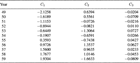
We have chosen an example based on aggregate data concerning import activity in the French economy. The data have been analyzed by Malinvaud (1968). Our discussion follows his presentation. The variables are imports (IMPORT), domestic production (DOPROD), stock formation (STOCK), and domestic consumption (CONSUM), all measured in billions of French francs for the years 1949 through 1966. The data are given in Table 9.5 and can be obtained from the book's Web site. The model being considered is

The regression results appear as Table 9.6. The index plot of residuals (Figure 9.3) shows a distinctive pattern, suggesting that the model is not well specified. Even though multicollinearity appears to be present (R² = 0.973 and all t-values small), it should not be pursued further in this model. Multicollinearity should only be attacked after the model specification is satisfactory. The difficulty with the model is that the European Common Market began operations in 1960, causing changes in import-export relationships. Since our objective in this chapter is to study the effects of multicollinearity, we shall not complicate the model by attempting to capture the behavior after 1959. We shall assume that it is now 1960 and look only at the 11 years 1949–1959. The regression results for those data are summarized in Table 9.7. The residual plot is now satisfactory (Figure 9.4).

Table 9.6 Import data (1949–1966): Regression Results

Figure 9.3 Import data (1949–1966): Index plot of the standardized residuals.

The value of R² = 0.99 is high. However, the coefficient of DOPROD is negative and not statistically significant, which is contrary to prior expectation. We believe that if STOCK and CONSUM were held constant, an increase in DOPROD would cause an increase in IMPORT, probably for raw materials or manufacturing equipment. Multicollinearity is a possibility here and in fact is the case. The simple correlation between CONSUM and DOPROD is 0.997. Upon further investigation it turns out that CONSUM has been about two-thirds of DOPROD throughout the 11-year period. The estimated relationship between the two quantities is

Table 9.7 Import data (1949–1959): Regression Results

Figure 9.4 Import data (1949–1959): Index plot of the standardized residuals.

Even in the presence of such severe multicollinearity the regression equation may produce some good forecasts. From Table 9.7, the forecasting equation is

Recall that the fit to the historical data is very good and the residual variation appears to be purely random. To forecast we must be confident that the character and strength of the overall relationship will hold into future periods. This matter of confidence is a problem in all forecasting models whether or not multicollinearity is present. For the purpose of this example we assume that the overall relationship does hold into future periods.² Implicit in this assumption is the relationship between DOPROD and CONSUM. The forecast will be accurate as long as the future values of DOPROD, STOCK, and CONSUM have the relationship that CONSUM is approximately equal to 0.7 × DOPROD.

For example, let us forecast the change in IMPORT next year corresponding to an increase in DOPROD of 10 units while holding STOCK and CONSUM at their current levels. The resulting forecast is

which means that IMPORT will decrease by −0.51 units. However, if the relationship between DOPROD and CONSUM is kept intact, CONSUM will increase by 10(2/3) = 6.67 units and the forecasted result is

IMPORT actually increases by 1.5 units, a more satisfying result and probably a better forecast. The case where DOPROD increases alone corresponds to a change in the basic structure of the data that were used to estimate the model parameters and cannot be expected to produce meaningful forecasts.

In summary, the two examples demonstrate that multicollinear data can seriously limit the use of regression analysis for inference and forecasting. Extreme care is required when attempting to interpret regression results when multicollinearity is suspected. In Section 9.4 we discuss methods for detecting extreme collinearity among predictor variables.

9.4 DETECTION OF MULTICOLLINEARITY

In the preceding examples some of the ideas for detecting multicollinearity were already introduced. In this section we review those ideas and introduce additional criteria that indicate collinearity. Multicollinearity is associated with unstable estimated regression coefficients. This situation results from the presence of strong linear relationships among the predictor variables. It is not a problem of misspecification. Therefore, the empirical investigation of problems that result from a collinear data set should begin only after the model has been satisfactorily specified. However, there may be some indications of multicollinearity that are encountered during the process of adding, deleting, and transforming variables or data points in search of the good model. Indication of multicollinearity that appear as instability in the estimated coefficients are as follows:

• Large changes in the estimated coefficients when a variable is added or deleted.
• Large changes in the coefficients when a data point is altered or dropped.

Once the residual plots indicate that the model has been satisfactorily specified, multicollinearity may be present if:

• The algebraic signs of the estimated coefficients do not conform to prior expectations; or
• Coefficients of variables that are expected to be important have large standard errors (small t-values).

For the IMPORT data discussed previously, the coefficient of DOPROD was negative and not significant. Both results are contrary to prior expectations. The effects of dropping or adding a variable can be seen in Table 9.8. There we see that the presence or absence of certain variables has a large effect on the other coefficients. For the EEO data (Tables 9.1 and 9.2) the algebraic signs are all correct, but their standard errors are so large that none of the coefficients are statistically significant. It was expected that they would all be important.

The presence of multicollinearity is also indicated by the size of the correlation coefficients that exist among the predictor variables. A large correlation between a pair of predictor variables indicates a strong linear relationship between those two variables. The correlations for the EEO data (Figure 9.2) are large for all pairs of predictor variables. For the IMPORT data, the correlation coefficient between DOPROD and CONSUM is 0.997.

The source of multicollinearity may be more subtle than a simple relationship between two variables. A linear relation can involve many of the predictor variables. It may not be possible to detect such a relationship with a simple correlation coefficient. As an example, we shall look at an analysis of the effects of advertising expenditures (A_t), promotion expenditures (P_t), and sales expense (E_t) on the aggregate sales of a firm in period t. The data represent a period of 23 years during which the firm was operating under fairly stable conditions. The data are given in Table 9.9 and can be obtained from the book's Web site.

Table 9.8 Import Data (1949–1959): Regression Coefficients for All Possible Regressions

The proposed regression model is

where A_t−1 and P_t−1 are the lagged one-year variables. The regression results are given in Table 9.10. The plot of residuals versus fitted values and the index plot of residuals (Figures 9.5 and 9.6), as well as other plots of the residuals versus the predictor variables (not shown), do not suggest any problems of misspecification. Furthermore, the correlation coefficients between the predictor variables are small (Table 9.11). However, if we do a little experimentation to check the stability of the coefficients by dropping the contemporaneous advertising variable A from the model, many things change. The coefficient of P_t drops from 8.37 to 3.70; the coefficients of lagged advertising A_t−1 and lagged promotions P_t−1 change signs. But the coefficient of sales expense is stable and R² does not change much.

The evidence suggests that there is some type of relationship involving the contemporaneous and lagged values of the advertising and promotions variables. The regression of A_t on P_t, A_t−1, and P_t−1 returns an R² of 0.973. The equation takes the form

Upon further investigation into the operations of the firm, it was discovered that close control was exercised over the expense budget during those 23 years of stability. In particular, there was an approximate rule imposed on the budget that the sum of A_t, A_t−1, P_t, and P_t−1 was to be held to approximately five units over every two-year period. The relationship

Figure 9.5 Standardized residuals versus fitted values of Sales.

Figure 9.6 Index plot of the standardized residuals.

Table 9.9 Annual Data on Advertising, Promotions, Sales Expenses, and Sales (Millions of Dollars)

is the cause of the multicollinearity.

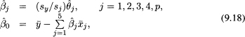
A thorough investigation of multicollinearity will involve examining the value of R² that results from regressing each of the predictor variables against all the others. The relationship between the predictor variables can be judged by examining a quantity called the variance inflation factor (VIF). Let be the square of the multiple correlation coefficient that results when the predictor variable X_j is regressed against all the other predictor variables. Then the variance inflation for X_j is

where p is the number of predictor variables. It is clear that if X_j has a strong linear relationship with the other predictor variables, would be close to 1, and VIF_j would be large. Values of variance inflation factors greater than 10 is often taken as a signal that the data have collinearity problems.

In absence of any linear relationship between the predictor variables (i.e., if the predictor variables are orthogonal), would be zero and VIF_j would be one. The deviation of VIF_j value from 1 indicates departure from orthogonality and tendency toward collinearity. The value of VIF_j also measures the amount by which the variance of the jth regression coefficient is increased due to the linear association of X_j with other predictor variables relative to the variance that would result if X_j were not related to them linearly. This explains the naming of this particular diagnostic.

Table 9.10 Regression Results for the Advertising Data

Table 9.11 Pairwise Correlation Coefficients for the Advertising Data

As tends toward 1, indicating the presence of a linear relationship in the predictor variables, the VIF for tends to infinity. It is suggested that a VIF in excess of 10 is an indication that multicollinearity may be causing problems in estimation.

The precision of an ordinary least squares (OLS) estimated regression coefficient is measured by its variance, which is proportional to σ², the variance of the error term in the regression model. The constant of proportionality is the VIF. Thus, the VIFs may be used to obtain an expression for the expected squared distance of the OLS estimators from their true values. Denoting the square of the distance by D², it can be shown that, on average,

This distance is another measure of precision of the least squares estimators. The smaller the distance, the more accurate are the estimates. If the predictor variables were orthogonal, the VIFs would all be 1 and D² would be pσ². It follows that the ratio

which shows that the average of the VIFs measures the squared error in the OLS estimators relative to the size of that error if the data were orthogonal. Hence, may also be used as an index of multicollinearity.

Most computer packages now furnish values of VIF_j, routinely. Some have built-in messages when high values of VIF_j are observed. In any regression analysis the values of VIF_j should always be examined to avoid the pitfalls resulting from fitting a regression model to collinear data by least squares.

In each of the three examples (EEO, Import, and Advertising) we have seen evidence of collinearity. The VIF_j's and their average values for these data sets are given in Table 9.12. For the EEO data the values of VIF_j range from 30.2 to 83.2, showing that all three variables are strongly intercorrelated and that dropping one of the variables will not eliminate collinearity. The average value of VIF of 50.3 indicates that the squared error in the OLS estimators is 50 times as large as it would be if the predictor variables were orthogonal.

For the Import data, the squared error in the OLS estimators is 313 times as large as it would be if the predictor variables were orthogonal. However, the VIF_j's indicate that domestic production and consumption are strongly correlated but are not correlated with the STOCK variable. A regression equation containing either CONSUM or DOPROD along with STOCK will eliminate collinearity.

Table 9.12 Variance Inflation Factors for Three Data Sets

For the Advertising data, VIF_E (for the variable E) is 1.1, indicating that this variable is not correlated with the remaining predictor variables. The VIF_j's for the other four variables are large, ranging from 26.6 to 44.1. This indicates that there is a strong linear relationship among the four variables, a fact that we have already noted. Here the prescription might be to regress sales S_t, against E_t, and three of the remaining four variables (A_t, P_t, A_t−1, S_t−1) and examine the resulting VIF_j's to see if collinearity has been eliminated.

9.5 CENTERING AND SCALING

The indicators of multicollinearity that have been described so far can all be obtained using standard regression computations. There is another, more unified way to analyze multicollinearity which requires some calculations that are not usually included in standard regression packages. The analysis follows from the fact that every linear regression model can be restated in terms of a set of orthogonal predictor variables. These new variables are obtained as linear combinations of the original predictor variables. They are referred to as the principal components of the set of predictor variables (Seber, 1984; Johnson and Wichern, 1992).

To develop the method of principal components, we may first need to center and/or scale the variables. We have been mainly dealing with regression models of the form

which are models with a constant term β₀. But we have also seen situations where fitting the no-intercept model

is necessary (see, e.g., Chapters 3 and 7). When dealing with constant term models, it is convenient to center and scale the variables, but when dealing with a no-intercept model, we need only to scale the variables.

9.5.1 Centering and Scaling in Intercept Models

If we are fitting an intercept model as in (9.6), we need to center and scale the variables. A centered variable is obtained by subtracting from each observation the mean of all observations. For example, the centered response variable is and the centered jth predictor variable is . The mean of a centered variable is zero. The centered variables can also be scaled. Two types of scaling are usually needed: unit length scaling and standardizing. Unit length scaling of the response variable Y and the jth predictor variable X_j, is obtained as follows:

where is the mean of, is the mean of X_j, and

The quantities L_y is referred to as the length of the centered variable because it measures the size or the magnitudes of the observations in . Similarly, L_j measure the length of the variable . The variables and , in (9.8) have zero means and unit lengths, hence this type of scaling is called unit length scaling.

In addition, unit length scaling has the following property:

That is, the correlation coefficient between the original variables, X_j and X_k, can be computed easily as the sum of the products of the scaled versions Z_j and Z_k.

The second type of scaling is called standardizing, which is defined by

where

are standard deviations of the response and jth predictor variable, respectively. The standardized variables and in (9.11) have means zero and unit standard deviations.

Since correlations are unaffected by shifting or scaling the data, it is both sufficient and convenient to deal with either the unit length scaled or the standardized versions of the variables. The variances and covariances of a set of p variables, X₁,…, X_p, can be neatly displayed as a squared array of numbers called a matrix. This matrix is known as the variance-covariance matrix. The elements on the diagonal that runs from the upper-left comer to the lower-right comer of the matrix are known as the diagonal elements. The elements on the diagonal of a variance-covariance matrix are the variances and the elements off the diagonal are the covariances.³ The variance-covariance matrix of the three predictor variables in the Import data for the years 1949–1959 is:

Thus, for example, Var(DOPROD) = 899.971, which is in the first diagonal element, and Cov(DOPROD, CONSUM) = 617.326, which is the value is the intersection of the first row and third column (or the third row and first column).

Similarly, the pairwise correlation coefficients can be displayed in matrix known as the correlation matrix. The correlation matrix of the three predictor variables in the Import data is:

This is the same as the variance-covariance matrix of the standardized predictor variables. Thus, for example, Cor(DOPROD, CONSUM) = 0.997, which indicates that the two variables are highly correlated. Note that all the diagonal elements of the correlation matrix are equal to one.

Recall that a set of variables is said to be orthogonal if there exists no linear relationships among them. If the standardized predictor variables are orthogonal, their matrix of variances and covariances consists of one for the diagonal elements and zero for the off-diagonal elements.

9.5.2 Scaling in No-Intercept Models

If we are fitting a no-intercept model as in (9.7), we do not center the data because centering has the effect of including a constant term in the model. This can be seen from:

rearranging terms, we obtain

where , Although a constant term does not appear in an explicit form in (9.14), it is clearly seen in (9.15). Thus, when we deal with no-intercept models, we need only to scale the data. The scaled variables are defined by:

where

The scaled variables in (9.16) have unit lengths but do not necessarily have means zero. Nor do they satisfy (9.10) unless the original variables have zero means.

We should mention here that centering (when appropriate) and/or scaling can be done without loss of generality because the regression coefficients of the original variables can be recovered from the regression coefficients of the transformed variables. For example, if we fit a regression model to centered data, the obtained regression coefficients are the same as the estimates obtained from fitting the model to the original data. The estimate of the constant term when using the centered data will always be zero. The estimate of the constant term for an intercept model can be obtained from:

Scaling, however, will change the values of the estimated regression coefficients. For example, the relationship between the estimates, , obtained from using the original data and the those obtained using the standardized data is given by

where and are the jth estimated regression coefficients obtained when using the original and standardized data, respectively. Similar formulas can be obtained when using unit length scaling instead of standardizing.

We shall make extensive use of the centered and/or scaled variables in the rest of this chapter and in Chapter 10.

9.6 PRINCIPAL COMPONENTS APPROACH

As we mentioned in the previous section, the principal components approach to the detection of multicollinearity is based on the fact that any set of p variables can be transformed to a set of p orthogonal variables. The new orthogonal variables are known as the principal components (PCs) and are denoted by C₁,…, C_p. Each variable C_j is a linear combination of the variables in (9.11). That is,

The linear combinations are chosen so that the variables C₁,…, C_p are orthogonal.⁴

The variance-covariance matrix of the PCs is of the form:

All the off-diagonal elements are zero because the PCs are orthogonal. The value on the jth diagonal element, λ_j is the variance of C_j, the jth PC. The PCs are arranged so that , that is, the first PC has the largest variance and the last PC has the smallest variance. The λ's are called eigenvalues of the correlation matrix of the predictor variables X₁,…, X_p. The coefficients involved in the creation of C_j in (9.19) can be neatly arranged in a column like

which is known as the eigenvector associated with the jth eigenvalue λ_j. If any one of the λ's is exactly equal to zero, there is a perfect linear relationship among the original variables, which is an extreme case of multicollinearity. If one of the λ's is much smaller than the others (and near zero), multicollinearity is present. The number of near zero λ's is equal to the number of different sets of multicollinearity that exist in the data. So, if there is only one near zero λ, there is only one set of multicollinearity; if there are two near zero λ's, there are two sets of different multicollinearity; and so on.

The eigenvalues of the correlation matrix in (9.13) are λ₁ = 1.999, λ₂ = 0.998, and λ₃ = 0.003. The corresponding eigenvectors are

Table 9.13 The PCs for the Import Data (1949–1959)

Thus, the PCs for the Import data for the years 1949–1959 are:

These PCs are given in Table 9.13. The variance-covariance matrix of the new variables is

The PCs lack simple interpretation since each is, in a sense, a mixture of the original variables. However, these new variables provide a unified approach for obtaining information about multicollinearity and serve as the basis of one of the alternative estimation techniques described in Chapter 10.

For the Import data, the small value of λ₃ = 0.003 points to multicollinearity. The other data sets considered in this chapter also have informative eigenvalues. For the EEO data, λ₁ = 2.952, λ₂ = 0.040, and λ₃ = 0.008. For the advertising data, λ₁ = 1.701, λ₂ = 1.288, λ₃ = 1.145, λ₄ = 0.859, and λ₅ = 0.007. In each case the presence of a small eigenvalue is indicative of multicollinearity.

A measure of the overall multicollinearity of the variables can be obtained by computing the condition number of the correlation matrix. The condition number is defined by

The condition number will always be greater than 1. A large condition number indicates evidence of strong collinearity. The harmful effects of collinearity in the data become strong when the values of the condition number exceeds 15 (which means that λ₁ is more than 225 times λ_p). The condition numbers for the three data sets EEO, Import, and advertising data are 19.20, 25.81, and 15.59, respectively. The cutoff value of 15 is not based on any theoretical considerations, but arises from empirical observation. Corrective action should always be taken when the condition number of the correlation matrix exceeds 30.

Another empirical criterion for the presence of multicollinearity is given by the sum of the reciprocals of the eigenvalues, that is,

If this sum is greater than, say, five times the number of predictor variables, multicollinearity is present.

One additional piece of information is available through this type of analysis. Since λ_j is the variance of the jth PC, if λ_j is approximately zero, the corresponding PC, C_j, is approximately equal to a constant. It follows that the equation defining the PC gives some idea about the type of relationship among the predictor variables that is causing multicollinearity. For example, in the Import data, λ₃ = 0.003 0. Therefore, C₃ is approximately constant. The constant is the mean value of C₃ which is zero. The PCs all have means of zero since they are linear functions of the standardized variables and each standardized variable has a zero mean. Therefore

Rearranging the terms yields

where the coefficient of (−0.007) has been approximated as zero. Equation (9.22) represents the approximate relationship that exists between the standardized versions of CONSUM and DOPROD. This result is consistent with our previous finding based on the high simple correlation coefficient (r = 0.997) between the predictor variables CONSUM and DOPROD. (The reader can confirm this high value of r by examining the scatter plot of CONSUM versus DOPROD.) Since λ₃ is the only small eigenvalue, the analysis of the PCs tells us that the dependence structure among the predictor variables as reflected in the data is no more complex than the simple relationship between CONSUM and DOPROD as given in Equation (9.22).

For the advertising data, the smallest eigenvalue is λ₅ = 0.007. The corresponding PC is

Setting C₅ to zero and solving for leads to the approximate relationship,

where we have taken the coefficient of to be approximately zero. This equation reflects our earlier findings about the relationship between A_t, P_t, A_t−1, and P_t−1. Furthermore, since λ₄ = 0.859 and the other λ's are all large, we can be confident that the relationship involving A_t, P_t, A_t−1, and P_t−1 in (9.24) is the only source of multicollinearity in the data.

Throughout this section, investigations concerning the presence of multicollinearity have been based on judging the magnitudes of various indicators, either a correlation coefficient or an eigenvalue. Although we speak in terms of large and small, there is no way to determine these threshold values. The size is relative and is used to give an indication either that everything seems to be in order or that something is amiss. The only reasonable criterion for judging size is to decide whether the ambiguity resulting from the perceived multicollinearity is of material importance in the underlying problem.

We should also caution here that the data analyzed may contain one or few observations that can have an undue influence on the various measures of collinearity (e.g., correlation coefficients, eigenvalues, or the condition number). These observations are called collinearity-influential observations. For more details the reader is referred to Hadi (1988).

9.7 IMPOSING CONSTRAINTS

We have noted that multicollinearity is a condition associated with deficient data and not due to misspecification of the model. It is assumed that the form of the model has been carefully structured and that the residuals are acceptable before questions of multicollinearity are considered. Since it is usually not practical and often impossible to improve the data, we shall focus our attention on methods of better interpretation of the given data than would be available from a direct application of least squares. In this section, rather than trying to interpret individual regression coefficients, we shall attempt to identify and estimate informative linear functions of the regression coefficients. Alternative estimating methods for the individual coefficients are treated in Chapter 10.

Before turning to the problem of searching the data for informative linear functions of the regression coefficients, one additional point concerning model specification must be discussed. A subtle step in specifying a relationship that can have a bearing on multicollinearity is acknowledging the presence of theoretical relationships among the regression coefficients. For example in the model for the Import data,

one may argue that the marginal effects of DOPROD and CONSUM are equal. That is, on the basis of economic reasoning, and before looking at the data, it is decided the β₁ = β₃ or equivalently, β₁ − β₃ = 0. As described in Section 3.9.3, the model in (9.25) becomes

Table 9.14 Regression Results of Import Data (1949–1959) with the constraint β₁ = β₃.

Figure 9.7 Index plot of the standardized residuals. Import data (1949–1959) with the constraint β₁ = β₃.

Thus, the common value of β₁ and β₃ is estimated by regressing IMPORT on STOCK and a new variable constructed as NEWVAR = DOPROD + CONSUM. The new variable has significance only as a technical manipulation to extract an estimate of the common value of β₁ and β₃. The results of the regression appear in Table 9.14. The correlation between the two predictor variables, STOCK and NEWVAR, is 0.0299 and the eigenvalues are λ₁ = 1.030 and λ₂ = 0.970. There is no longer any indication of multicollinearity. The residual plots against time and the fitted values indicate that there are no other problems of specification (Figures 9.7 and 9.8, respectively). The estimated model is

Note that following the methods outlined in Section 3.9.3, it is also possible to test the constraint, β₁ = β₃, as a hypothesis. Even though the argument for β₁ = β₃ may have been imposed on the basis of existing theory, it is still interesting to evaluate the effect of the constraint on the explanatory power of the full model. The values of R² for the full and restricted models are 0.992 and 0.987, respectively. The F-ratio for testing H₀(β₁ = β₃) is 3.36 with 1 and 8 degrees of freedom. Both results suggest that the constraint is consistent with the data.

Figure 9.8 Standardized residuals against fitted values of Import data (1949–1959) with the constraint β₁ = β₃.

The constraint that β₁ = β₃ is, of course, only one example of the many types of constraints that may be used when specifying a regression model. The general class of possibilities is found in the set of linear constraints described in Chapter 3. Constraints are usually justified on the basis of underlying theory. They may often resolve what appears to be a problem of multicollinearity. In addition, any particular constraint may be viewed as a testable hypothesis and judged by the methods described in Chapter 3.

9.8 SEARCHING FOR LINEAR FUNCTIONS OF THE β's

We assume that the model

has been carefully specified so that the regression coefficients appearing are of primary interest for policy analysis and decision making. We have seen that the presence of multicollinearity may prevent individual β's from being accurately estimated. However, as demonstrated below, it is always possible to estimate some linear functions of the β's accurately (Silvey, 1969). The obvious questions are: Which linear functions can be estimated, and of those that can be estimated, which are of interest in the analysis? In this section we use the data to help identify those linear functions that can be accurately estimated and, at the same time, have some value in the analysis.

Table 9.15 Regression Results When Fitting Model (9.26) to the Import Data (1949–1959)

First we shall demonstrate in an indirect way that there are always linear functions of the β's that can be accurately estimated.⁵ Consider once again the Import data. We have argued that there is a historical relationship between CONSUM and DOPROD that is approximated as CONSUM = (2/3) DOPROD. Replacing CONSUM in the original model,

Equivalently stated, by dropping CONSUM from the equation we are able to obtain accurate estimates of β₁ + (2/3)β₃ and β₂. Multicollinearity is no longer present. The correlation between DOPROD and STOCK is 0.026. The results are given in Table 9.15. R² is almost unchanged and the residual plots (not shown) are satisfactory. In this case we have used information in addition to the data to argue that the coefficient of DOPROD in the regression of IMPORT on DOPROD and STOCK is the linear combination β₁ + (2/3)β₃. Also, we have demonstrated that this linear function can be estimated accurately even though multicollinearity is present in the data. Whether or not it is useful to know the value of β₁ + (2/3)β₃, of course, is another question. At least it is important to know that the estimate of the coefficient of DOPROD in this regression is not measuring the pure marginal effect of DOPROD, but includes part of the effect of CONSUM.

The above example demonstrates in an indirect way that there are always linear functions of the β's that can be accurately estimated. However, there is a constructive approach for identifying the linear combinations of the β's that can be accurately estimated. We shall use the advertising data introduced in Section 9.4 to demonstrate the method. The concepts are less intuitive than those found in the other sections of the chapter. We have attempted to keep things simple. A formal development of this problem is given in the Appendix to this chapter.

We begin with the linear transformation introduced in Section 9.6 that takes the standardized predictor variables into a new orthogonal set of variables. The standardized versions of the five predictor variables are denoted by . The standardized response variable, sales, is denoted by . The transformation that takes X₁,…, X₅ into the new set of orthogonal variables C₁,…, C₅ is

The coefficients in the equation defining C₁ are the components of the eigenvector corresponding to the largest eigenvalue of the correlation matrix of the predictor variables. Similarly, the coefficients defining C₂ through C₅ are components of the eigenvectors corresponding to the remaining eigenvalues in order by size. The variables C₁,…, C₅ are the PCs associated with the standardized versions of the predictors variables, as described in the preceding Section 9.6.

The regression model stated, as given in (9.4) in terms of the original variables is

In terms of standardized variables, the equation is written as

where denotes the standardized version of the variable A_t. The regression coefficients in Equation (9.29) are often referred to as the beta coefficients. They represent marginal effects of the predictor variables in standard deviation units. For example, θ₁ measures the change in standardized units of sales (S) corresponding to an increase of one standard deviation unit in advertising (A).

Let be the least squares estimate of when model (9.28) is fit to the data. Similarly, let be the least squares estimate of obtained from fitting model (9.29). Then and are related by

where is the mean of Y and s_y and s_j are standard deviations of the response and jth predictor variable, respectively.

Equation (9.29) has an equivalent form, given as

The equivalence of Equations (9.29) and (9.31) results from the relationship between the 's and C's in Equations (9.27) and the relationship between the α's and θ's and their estimated values, 's and 's, given as

Note that the transformation involves the same weights that are used to define Equation (9.27). The advantage of the transformed model is that the PCs are orthogonal. The precision of the estimated regression coefficients as measured by the variance of the 's is easily evaluated. The estimated variance of is . It is inversely proportional to the ith eigenvalue. All but ₅ may be accurately estimated since only λ₅ is small. (Recall that λ₁ = 1.701, λ₂ = 1.288, λ₃ = 1.145, λ₄ = 0.859, and λ₅ = 0.007.)

Our interest in the 's is only as a vehicle for analyzing the 's. From the representation of Equation (9.32) it is a simple matter to compute and analyze the variances and, in turn, the standard errors of the 's. The variance of is

where v_ij is the coefficient of in the j Equation in (9.32). Since the estimated variance of , where is the residual mean square, (9.33) becomes

For example, the estimated variance of is

Recall that and only λ₅ is small, (λ₅ = 0.007). Therefore, it is only the last term in the expression for the variance that is large and could destroy the precision of . Since expressions for the variances of the other 's are similar to Equation (9.35), a requirement for small variance is equivalent to the requirement that the coefficient of 1/λ₅ be small. Scanning the equations that define the transformation from to , we see that is the most precise estimate since the coefficient of 1/λ₅ in the variance expression for is (−0.01)² = 0.0001.

Expanding this type of analysis, it may be possible to identify meaningful linear functions of the θ's that can be more accurately estimated than individual θ's. For example, we may be more interested in estimating θ₁ − θ₂ than θ₁ and θ₂ separately. In the sales model, θ₁ − θ₂ measures the increment to sales that corresponds to increasing the current year's advertising budget, X₁, by one unit and simultaneously reducing the current year's promotions budget, X₂, by one unit. In other words, θ₁ − θ₂ represents the effect of a shift in the use of resources in the current year. The estimate of θ₁ − θ₂ is . The variance of this estimate is obtained simply by subtracting the equation for and in (9.32) and using the resulting coefficients of the 's as before. That is,

from which we obtain the estimated variance of () as

or, equivalently, as

The small coefficient of 1/λ₅ makes it possible to estimate accurately. Generalizing this procedure we see that any linear function of the 's that results in a small coefficient for 1/λ₅ in the variance expression can be estimated with precision.

9.9 COMPUTATIONS USING PRINCIPAL COMPONENTS

The computations required for this analysis involve something in addition to a standard least squares computer program. The raw data must be processed through a principal components subroutine that operates on the correlation matrix of the predictor variables in order to compute the eigenvalues and the transformation weights found in Equations (9.32). Most regression packages produce the estimated beta coefficients as part of the standard output.

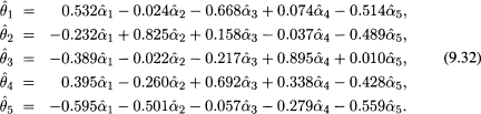
For the advertising data, the estimates can be computed in two equivalent ways. They can be obtained directly from a regression of the standardized variables as represented in Equation (9.29). The results of this regression are given in Table 9.16. Alternatively, we can fit the model in (9.31) by the least squares regression of the standardized response variable on the the five PCs and obtain the estimates . The results of this regression are shown in Table 9.17. Then, we use (9.32) to obtain . For example,

Using the coefficients in (9.32), the standard error of can be computed. For example the estimated variance of is

Table 9.16 Regression Results Obtained From Fitting the Model in (9.29)

Table 9.17 Regression Results Obtained From Fitting the Model in (9.31)

which means that the standard error of is

It should be noted that the t-values for testing and equal to zero are identical. The beta coefficient, is a scaled version of . When constructing t-values as either /s.e.(), or / s.e.(), the scale factor is canceled.

The estimate of is 0.583 −0.973 = −0.390. The variance of can be computed from Equation (9.36) as 0.008. A 95% confidence interval for is or −0.58 to −0.20. That is, the effect of shifting one unit of expenditure from promotions to advertising in the current year is a loss of between 0.20 and 0.58 standardized sales unit.

There are other linear functions that may also be accurately estimated. Any function that produces a small coefficient for 1/λ₅ in the variance expression is a possibility. For example, Equations (9.31) suggest that all differences involving , and can be considered. However, some of the differences are meaningful in the problem, whereas others are not. For example, the difference () is meaningful, as described previously. It represents a shift in current expenditures from promotions to advertising. The difference is not particularly meaningful. It represents a shift from current advertising expenditure to a previous year's advertising expenditure. A shift of resources backward in time is impossible. Even though could be accurately estimated, it is not of interest in the analysis of sales.

In general, when the weights in Equation (9.32) are displayed and the corresponding values of the eigenvalues are known, it is always possible to scan the weights and identify those linear functions of the original regression coefficients that can be accurately estimated. Of those linear functions that can be accurately estimated, only some will be of interest for the problem being studied.

To summarize, where multicollinearity is indicated and it is not possible to supplement the data, it may still be possible to estimate some regression coefficients and some linear functions accurately. To investigate which coefficients and linear functions can be estimated, we recommend the analysis (transformation to principal components) that has just been described. This method of analysis will not overcome multicollinearity if it is present. There will still be regression coefficients and functions of regression coefficients that cannot be estimated. But the recommended analysis will indicate those functions that are estimable and indicate the structural dependencies that exist among the predictor variables.

9.10 BIBLIOGRAPHIC NOTES

The principal components techniques used in this chapter are derived in most books on multivariate statistical analysis. It should be noted that principal components analysis involves only the predictor variables. The analysis is aimed at characterizing and identifying dependencies (if they exist) among the predictor variables. For a comprehensive discussion of principal components, the reader is referred to Johnson and Wichern (1992) or Seber (1984). Several statistical software packages are now commercially available to carry out the analysis described in this chapter.

EXERCISES

9.1  In the analysis of the Advertising data in Section 9.4 it is suggested that the regression of sales S_t against E_t and three of the remaining four variables (A_t, P_t, A_t−1, S_t−1) may resolve the collinearity problem. Run the four suggested regressions and, for each of them, examine the resulting VIF_j's to see if collinearity has been eliminated.

9.2 Gasoline Consumption: To study the factors that determine the gasoline consumption of cars, data were collected on 30 models of cars. Besides the gasoline consumption (Y), measured in miles per gallon for each car, 11 other measurements representing physical and mechanical characteristics are given. The source of the data in Table 9.19 is Motor Trend magazine for the year 1975. Definitions of variables are given in Table 9.18. We wish to determine whether the data set is collinear.

(a) Compute the correlation matrix of the predictor variables X₁,…, X₁₁ and the corresponding pairwise scatter plots. Identify any evidence of collinearity.

(b) Compute the eigenvalues, eigenvectors, and the condition number of the correlation matrix. Is multicollinearity present in the data?

(c) Identify the variables involved in multicollinearity by examining the eigenvectors corresponding to small eigenvalues.

(d) Regress Y on the 11 predictor variables and compute the VIP for each of the predictors. Which predictors are affected by the presence of collinearity?

9.3 Refer to the Presidential Election Data in Table 5.17 and consider fitting a model relating V to all the variables (including a time trend representing year of election) plus as many interaction terms involving two or three variables as you possibly can.

(a) What is the maximum number of terms (coefficients) in a linear regression model that you can fit to these data? [Hint: Consider the number of observations in the data.]

(b) Examine the predictor variables in the above model for the presence of multicollinearity. (Compute the correlation matrix, the condition number, and the VIFs.)

(c) Identify the subsets of variables involved in collinearity. Attempt to solve the multicollinearity problem by deleting some of the variables involved in multicollinearity.

(d) Fit a model relating V to the set of predictors you found to be free from multicollinearity.

Appendix: Principal Components

In this appendix we present the principal components approach to the detection of multicollinearity using matrix notation.

A. The Model

The regression model can be expressed as

where Y is an n × 1 vector of observations on the response variable, Z = (Z₁,…,Z_p) is an n × p matrix of n observations on p predictor variables, θ is a p × 1 vector of regression coefficients and ε is an n × 1 vector of random errors. It is assumed that E(ε) = 0, E(εε^T) = σ²I, where I is the identity matrix of order n. It is also assumed, without loss of generality, that Y and Z have been centered and scaled so that Z^TZ and Z^TY are matrices of correlation coefficients.

Table 9.18 Variables for the Gasoline Consumption Data in Table 9.19

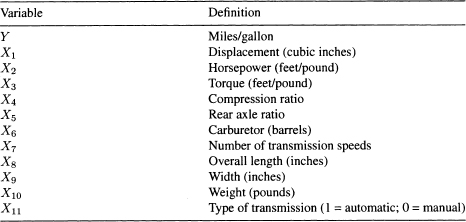
Table 9.19 Gasoline Consumption and Automotive Variables.

There exist square matrices, Λ and V satisfying⁶

The matrix Λ is diagonal with the ordered eigenvalues of Z^TZ on the diagonal. These eigenvalues are denoted by . The columns of V are the normalized eigenvectors corresponding to λ₁,…, λ_p. Since VV^T = I, the regression model in (A.1) can be restated in terms of the PCs as

where

The matrix C contains p columns C₁,…, C_p, each of which is a linear functions of the predictor variables Z₁,…, Z_p. The columns of C are orthogonal and are referred to as principal components (PCs) of the predictor variables Z₁,…, Z_p. The columns of C satisfy and .

The PCs and the eigenvalues may be used to detect and analyze collinearity in the predictor variables. The restatement of the regression model given in Equation (A.3) is a reparameterization of Equation (A.1) in terms of orthogonal predictor variables. The λ's may be viewed as sample variances of the PCs. If λ_i = 0, all observations on the ith PC are also zero. Since the jth PC is a linear function of Z₁,…, Z_p, when λ_j = 0 an exact linear dependence exists among the predictor variables. It follows that when λ_j is small (approximately equal to zero) there is an approximate linear relationship among the predictor variables. That is, a small eigenvalue is an indicator of multicollinearity. In addition, from Equation (A.4) we have

which identifies the exact form of the linear relationship that is causing the multicollinearity.

B. Precision of Linear Functions of

Denoting it and as the least squares estimators for α and θ, respectively, it can be shown that , and conversely, . With , it follows that the variance-covariance matrix of is , and the corresponding matrix for is . Let L be an arbitrary p × 1 vector of constants. The linear function has least squares estimator and variance

Let V_j be the jth column of V. Then L can be represented as

for appropriately chosen constants r₁,…, r_p. Then (A.5) becomes or, equivalently,

where Λ⁻¹ is the inverse of Λ.

To summarize, the variance of is a linear combination of the reciprocals of the eigenvalues. It follows that will have good precision either if none of the eigenvalues are near zero or if is at most the same magnitude as when is small. Furthermore, it is always possible to select a vector, L, and thereby a linear function of , so that the effect of one or few small eigenvalues is eliminated and has a small variance. Refer to Silvey (1969) for a more complete development of these concepts.