
CHAPTER 12
LOGISTIC REGRESSION
12.1 INTRODUCTION
In our discussion of regression analysis so far the response variable Y has been regarded as a continuous quantitative variable. The predictor variables, however, have been both quantitative, as well as qualitative. Indicator variables, which we have described earlier, fall into the second category. There are situations, however, where the response variable is qualitative. In this chapter we present methods for dealing with this situation. The methods presented in this chapter are very different from the method of least squares considered in earlier chapters.
Consider a procedure in which individuals are selected on the basis of their scores in a battery of tests. After five years the candidates are classified as “good” or “poor”. We are interested in examining the ability of the tests to predict the job performance of the candidates. Here the response variable, performance, is dichotomous. We can code “good” as 1 and “poor” as 0, for example. The predictor variables are the scores in the tests.
In a study to determine the risk factors for cancer, health records of several people were studied. Data were collected on several variables, such as age, sex, smoking, diet, and the family's medical history. The response variable was, the person had cancer (Y = 1), or did not have cancer (Y = 0).
In the financial community the “health” of a business is of primary concern. The response variable is solvency of the firm (bankrupt = 0, solvent = 1), and the predictor variables are the various financial characteristics associated with the firm. Situations where the response variable is a dichotomous variable are quite common and occur extensively in statistical applications.
12.2 MODELING QUALITATIVE DATA
The qualitative data with which are dealing, the binary response variable, can always be coded as having two values, 0 or 1. Rather than predicting these two values we try to model the probabilities that the response takes one of these two values. The limitation of the previously considered standard linear regression model is obvious.
We illustrate this point by considering a simple regression problem, in which we have only one predictor. The same considerations hold for the multiple regression case. Let π denote the probability that Y = 1 when X = x. If we use the standard linear model to describe π, then our model for the probability would be
Since π is a probability it must lie between 0 and 1. The linear function given in (12.1) is unbounded, and hence cannot be used to model probability. There is another reason why ordinary least squares method is unsuitable. The response variable Y is a binomial random variable, consequently its variance will be a function of π, and depends on X. The assumption of equal variance (homoscedasticity) does not hold. We could use the weighted least squares, but there are problems with that approach. The values of π are not known. In order to use weighted least squares approach, we will have to start with an initial guess for the value of π, and then iterate. Instead of this complex method we will describe an alternative method for modeling probabilities.
12.3 THE LOGIT MODEL
The relationship between the probability π and X can often be represented by a logistic response function. It resembles a S-shaped curve, a sketch of which is given in Figure 12.1. The probability π initially increases slowly with increase in X, then the increase accelerates, finally stabilizes, but does not increase beyond 1. Intuitively this makes sense. Consider the probability of a questionnaire being returned as a function of cash reward, or the probability of passing a test as a function of the time put in studying for it.
The shape of the S-curve given in Figure 12.1 can be reproduced if we model the probabilities as follows:

Figure 12.1 Logistic response function.
where e is the base of the natural logarithm. The probabilities here are modeled by the distribution function (cumulative probability function) of the logistic distribution. There are other ways of modeling the probabilities that would also produce the S-curve. The cumulative distribution of the normal curve has also been used. This gives rise to the probit model. We will not discuss the probit model here, as we consider the logistic model simpler and superior to the probit model.
The logistic model can be generalized directly to the situation where we have several predictor variables. The probability π is modeled as

The equation in (12.3) is called the logistic regression function. It is nonlinear in the parameters β0, β1,…, βp. However, it can be linearized by the logit transformation.1 Instead of working directly with π we work with a transformed value of π. If π is the probability of an event happening, the ratio π/(1 − π) is called the odds ratio for the event. Since
![]()
then
Taking the natural logarithm of both sides of (12.4), we obtain

The logarithm of the odds ratio is called the logit. It can be seen from (12.5) that the logit transformation produces a linear function of the parameters β0, β1,…, βp. Note also that while the range of values of π in (12.3) is between 0 and 1, the range of values of log(π/(1 − π)) is between −∞ and +∞, which makes the logits (the logarithm of the odds ratio) more appropriate for linear regression fitting.
Modeling the response probabilities by the logistic distribution and estimating the parameters of the model given in (12.3) constitutes fitting a logistic regression. In logistic regression the fitting is carried out by working with the logits. The logit transformation produces a model that is linear in the parameters. The method of estimation used is the maximum likelihood method. The maximum likelihood estimates are obtained numerically, using an iterative procedure. Unlike least squares fitting, no closed-form expression exists for the estimates of the parameters. We will not go into the computational aspects of the problem but refer the reader to McCullagh and Nelder (1983), Seber (1984), and Hosmer and Lemeshow (1989).
To fit a logistic regression in practice a computer program is essential. Most regression packages have a logistic regression option. After the fitting one looks at the same set of questions that are usually considered in linear regression. Questions about the suitability of the model, the variables to be retained, and goodness of fit are all considered. Tools used are not the usual R2, t, and F tests, the ones employed in least squares regression, but others which provide answers to these same questions. Hypothesis testing is done by different methods, since the method of estimation is maximum likelihood as opposed to least squares. Information Criteria such as AIC and BIC can be used for model selection. Instead of SSE, the logarithm of the likelihood for the fitted model is used. An explicit formula is given in Section 12.6.
12.4 EXAMPLE: ESTIMATING PROBABILITY OF BANKRUPTCIES
Detecting ailing financial and business establishments is an important function of audit and control. Systematic failure to do audit and control can lead to grave consequences, such as the savings-and-loan fiasco of the 1980s in the United States. Table 12.1 gives some of the operating financial ratios of 33 firms that went bankrupt after 2 years and 33 that remained solvent during the same period. The data can also be found in the book's Web site.2 A multiple logistic regression model is fitted using variables Xl, X2, and X3. The output from fitting the model is given in Table 12.2.
Three financial ratios were available for each firm:

The response variable is defined as
![]()
Table 12.2 has a certain resemblance to the standard regression output. Some of the output serve similar functions. We now describe and interpret the output obtained from fitting a logistic regression. If π denotes the probability of a firm remaining solvent after 2 years, the fitted logit is given by:
This corresponds to the fitted regression equation in standard analysis. Here instead of predicting Y we obtain a model to predict the logits, log(π/(1 − π)). From the logits, after transformation, we can get the predicted probabilities. The constant and the coefficients are read directly from the second column in the table. The standard errors (s.e.) of the coefficients are given in the third column. The fourth column headed by Z is the ratio of the coefficient and the standard deviation. The Z is sometimes referred to as the Wald Statistic (Test). The Z corresponding to the coefficient of X2 is obtained from dividing 0.181 by 0.107. In the standard regression this would be the t-test, This ratio for the logistic regression has a normal distribution as opposed to a t-distribution that we get in linear regression. The fifth column gives the p-value corresponding to the observed Z value, and should be interpreted like any p-value (see Chapters 2 and 3). These p-values are used to judge the significance of the coefficient. Values smaller than 0.05 would lead us to conclude that the coefficient is significantly different from 0 at the 5% significance level. From the p-values in Table 12.2, we see that none of the variables individually are significant for predicting the logits of the observations.
In the standard regression output the regression coefficients have a simple interpretation. The regression coefficient of the jth predictor variable Xj is the expected change in Y for unit change in Xj when other variables are held fixed. The coefficient of X2 in (12.6) is the expected change in the logit for unit change in X2 when the other variables are held fixed. The coefficients of a logistic regression fit have another interpretation that is of major practical importance. Keeping Xl and X3 fixed, for unit increase in X2 the relative odds of
![]()
is multiplied by ![]() , that is there is an increase of 20%. These values for each of the variables is given in the sixth column headed by Odds Ratio. They represent the change in odds ratio for unit change of a particular variable while the others are held constant. The change in odds ratio for unit change in variable Xj, while the other variables are held fixed, is
, that is there is an increase of 20%. These values for each of the variables is given in the sixth column headed by Odds Ratio. They represent the change in odds ratio for unit change of a particular variable while the others are held constant. The change in odds ratio for unit change in variable Xj, while the other variables are held fixed, is ![]() . If Xj was a binary variable, taking values 1 or 0, then
. If Xj was a binary variable, taking values 1 or 0, then ![]() would be the actual value of the odds ratio rather than the change in the value of the odds ratio.
would be the actual value of the odds ratio rather than the change in the value of the odds ratio.
Table 12.1 Financial Ratios of Solvent and Bankrupt Firms

Table 12.2 Output from the Logistic Regression Using X1, X2, and X3

The 95% confidence intervals of the odds ratios are given in the last two columns of the table. If the confidence interval does not contain the value 1 the variable has a significant effect on the odds ratio. If the interval is below 1 the variable lowers significantly the relative odds. On the other hand, if the interval lies above 1 the relative odds is significantly increased by the variable.
To see whether the variables collectively contribute in explaining the logits a test that examines whether the coefficients β1,…, βp are all zero is performed. This corresponds to the case in multiple regression analysis where we test whether all the regression coefficients can be taken to be zero. The statistic G given at the bottom of Table 12.2 performs that task. The statistic G has a chi-square distribution. The p-value is considerably smaller than .05, and indicates that the variables collectively influence the logits.
12.5 LOGISTIC REGRESSION DIAGNOSTICS
After fitting a logistic regression model certain diagnostic measures can be examined for the detection of outliers, high leverage points, influential observations, and other model deficiencies. The diagnostic measures developed in Chapter 4 for the standard linear regression model can be adapted to the logistic regression model. Regression packages with a logistic regression option usually give various diagnostic measures. These include:
- The estimated probabilities
 .
. - One or more types of residuals, for example, the standardized deviance residuals, DRi, and the standardized Personian residuals, PRi, i = 1,…, n.
- The weighted leverages,
 , which measure the potential effects of the observations in the predictor variables on the obtained logistic regression results.
 - The scaled difference in the regression coefficients when the ith observation is deleted: DBETAi, i = 1,…, n.
- The change in the chi-squared statistics G when the ith observation is deleted: DFGi, i = 1,…, n.
The formulas and derivations of these measures are beyond the scope of this book. The interested reader is referred to Pregibon (1981), Landwehr, Pregibon, and Shoemaker (1984), Hosmer and Lemeshow (1989) and the references therein. The above measures, however, can be used in the same way as the corresponding measures obtained from a linear fit (Chapter 4). For example, the following graphical displays can be examined:
- The scatter plot of DRi versus
 .
. - The scatter plot of PRi versus .
- The index plots of DRi, DBETAi, DGi, and .
As an illustrative example using the Bankruptcy data, the index plots of DRi, DBETAi, and DGi obtained from the fitted logistic regression model in (12.6), are shown in Figures (12.2), (12.3), and (12.4), respectively. It can easily be seen from these graphs that observations 9, 14, 52, and 53 are unusual and that they may have undue influence on the logistic regression results. We leave it as an exercise for the reader to determine if their deletion would make a significant difference in the results and the conclusion drawn from the analysis.
12.6 DETERMINATION OF VARIABLES TO RETAIN
In the analysis of the Bankruptcy data we have determined so far that the variables X1, X2, and X3, collectively have explanatory power. Do we need all three variables? This is analogous to the problem of variable selection in multiple regression that was discussed in Chapter 11. Instead of looking at the reduction in the error sum of squares we look at the change in the likelihood (more precisely, the logarithm of the likelihood) for the two fitted models. The reason for this is that in logistic regression the fitting criterion is the likelihood, whereas in least squares it is the sum of squares. Let L(p) denote the logarithm of the likelihood when we have a model with p variables and a constant. Similarly, let L(p + q) be the logarithm of the likelihood for a model in which we have p + q variables and a constant. To see whether the q additional variables contribute significantly we look at 2(L(p + q) − L(p)). This quantity is twice the difference between the log-likelihood for the two models. This difference is distributed as a chi-square variable with q degrees of freedom (see Table A.3).
The magnitude of this quantity determines the significance of the test. A small value of chi-square would lead to the conclusion that the q variables do not add significantly to the improvement in prediction of the logits, and is therefore not necessary in the model. A large value of chi-square would call for the retention of the q variables in the model. The critical value is determined by the significance level of the test. This test procedure is valid when n, the number of observations available for fitting the model, is large.

Figure 12.2 Bankruptcy data: Index plot of DRi, the standardized deviance residuals.

Figure 12.3 Bankruptcy data: Index plot of DBETAi, the scaled difference in the regression coefficients when the ith observation is deleted.
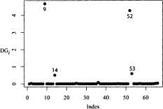
Figure 12.4 Bankruptcy data: Index plot of DGi, the change in the chi-squared statistics G when the ith observation is deleted.
An idea of the predictive power of a variable for possible inclusion in the logistic model can be obtained from a simple graphical plot. Side-by-side boxplots are constructed for each of the explanatory variable. Side-by-side boxplot will indicate the variables that may be useful for this purpose. Variables with boxplots different for the two groups are likely candidates. Note that this does not take into account the correlation between the variables. The formal procedure described above takes into account the correlations. With a large number of explanatory variables the boxplots provide a quick screening procedure.
Table 12.3 Output From the Logistic Regression Using X1 and X2

Table 12.4 Output From the Logistic Regression Using X1

In the Bankruptcy data we are analyzing, let us see if the variable X3 can be deleted without degrading the model. We want to answer the question: Should the variable X3 be retained in the model? We fit a logistic regression using X1 and X2. The results are given in Table 12.3. The log-likelihood for the model with X1, X2, and X3 is −2.906, whereas with only X1 and X2 it is −4.736. Here p = 2 and q = 1, and 2(L(3) − L(2)) = 3.66. This is a chi-square variable with 1 degree of freedom. From Table A.3, we find that the 5% critical value of the chi-square distribution with 1 degree of freedom is 3.84. At the 5% level we can conclude that the variable X3 can be deleted without affecting the effectiveness of the model.
Let us now see if we can delete X2. The result of regressing Y on X1 is given in Table 12.4. The resulting log-likelihood is −7.902. The test statistic, which we have described earlier, has a value of 6.332. This is distributed as a chi-square random variable with 1 degree of freedom. The 5% value, as we saw earlier, was 3.84. The analysis indicates that we should not delete X2 from our model. The p-value for this test, as can be verified, is 0.019. To predict probabilities of bankruptcies of firms in our data we should include both X1 and X2 in our model.
The procedure that we have outlined above enables us to test any nested model. A set of models are said to be nested if they can be obtained from a larger model as special cases. The methodology is similar to that used in analyzing nested models in multiple regression. The only difference is that here our test statistic is based on log of the likelihood instead of sum of squares.
Table 12.5 The AIC and BIC Criteria for Various Logistic Regression models

The AIC and BIC criteria discussed in Section 11.5.3 can be used to judge the suitability of various logistic models, and thereby the desirability of retaining a variable in the model. In the context of p-term logistic logistic regression, AIC and BIC are:
where p denotes the number of variables in the model. Table 12.5 shows AIC and BIC for all possible models. The best AIC model is the one that includes all three variables (lowest AIC). While BIC picks X1 X2 as the best model, but the one containing all three variables is equally adequate. The BIC for the two top models differ by less than 2.
12.7 JUDGING THE FIT OF A LOGISTIC REGRESSION
The overall fit of a multiple regression model is judged, for example, by the value of R2 from the fitted model. No such simple satisfactory measure exists for logistic regression. Some ad hoc measures have been proposed which are based on the ratio of likelihoods. Most of these are functions of the ratio of the likelihood for the model and the likelihood of the data under a binomial model. These measures are not particularly informative and we will consider a different approach.
The logistic regression equation attempts to model probabilities for the two values of Y (0 or 1). To judge how well the model is doing we will determine the number of observations in the sample that the model is classifying correctly. Our approach will be to fit the logistic model to the data, and calculate the fitted logits. From the fitted logits we will calculate the fitted probabilities for each observation. If the fitted probability for an observation is greater than 0.5 we will assign it to Group 1(Y = 1), and ifless than 0.5 we will classify it in Group 0 (Y = 0). We will then determine what proportion of the data is classified correctly. A high proportion of correct classification will indicate to us that the logistic model is working well. A low proportion of correct classification will indicate poor performance.
Different cutoff values, other than 0.5, have been suggested in the literature. In most practical situations, without any auxiliary information, such as the relative cost of misclassification or the relative frequency of the two categories in the population, 0.5 is recommended as a cutoff value.
A slightly more problematical question is how high the correct classification probability has to be before logistic regression is thought to be effective. Suppose that in sample of size n there are n1 observations from Group 1, and n2 from Group 2. If we classify all the observations into one group or the other, then we will get either n1/n or n2/n proportions of observations classified correctly. As a base level for correct classification we can take the max(n1/n, n2/n). The proportion of observation classified correctly by the logistic regression should be much higher than the base level for the logistic model to be deemed useful.
For the Bankruptcy data that we have been analyzing logistic regression performs very well. Using variables Xl and X2, we find that the model misclassifies one observation from the solvent group (observation number 36), and one observation from the bankruptcy group (observation number 9). The overall correct classification rate (64/66) = 0.97. This is considerably higher than the base level rate of 0.5.
The concept of overall correct classification for the observed sample to judge the adequacy of the logistic model that we have discussed has been generalized. This generalization is used to produce a statistic to judge the fit of the logistic model. It is sometimes called the Concordance Index and is denoted by C. This statistic is calculated by considering all possible pairs formed by taking one observation from each group. Each of the pairs is then classified by using the fitted model. The Concordance Index is the percent of all possible pairs that is classified correctly. Thus, C lies between 0.5 and 1. Values of C close to 0.5 shows the logistic model performing poorly (no better than guessing). The value of C for the logistic model with X1X2X3 is 0.99. Several currently available software computes the value of C.
The observed correct classification rate should be treated with caution. In practice, if this logistic regression was applied to a new set of observations from this population, it would be very unlikely to do as well. The classification probability has an upward bias. The bias arises due to the fact that the same data that were used to fit the model, was used to judge the performance of the model. The model fitted to a given body of data is expected to perform well on the same body of data. The true measure of the performance of the logistic regression model for classification is the probability of classifying a future observation correctly and not a sample observation. This upward bias in the estimate of correct classification probability can be reduced by using resampling methods, such as jack-knife or bootstrap. These will not be discussed here. The reader is referred to Efron (1982) and Diaconis and Efron (1983).
12.8 THE MULTINOMIAL LOGIT MODEL
In our discussion of logistic regression we have so far assumed that the qualitative response variable assumes only two values, generically, 1 for success and 0 for failure. The logistic regression model can be extended to situations where the response variable assumes more than two values. In a study of the choice of mode of transportation to work, the response variable may be private automobile, car pool, public transport, bicycle, or walking. The response falls into five categories. There is no natural ordering of the categories. We might want to analyze how the choice is related to factors such as age, sex, income, distance traveled, etc. The resulting model can be analyzed by using slightly modified methods that were used in analyzing the dichotomous outcomes. This method is called the multinomial (polytomous) logistic regression.
The response categories are not ordered in the example described above. There are situations where the response categories are ordered. In an opinion survey, the response categories might be, strongly agree, agree, no opinion, disagree, and strongly disagree. The response categories are naturally ordered. In a clinical trial the responses to a treatment could be classified as improved, no change, worse. For these situations a different method called the Proportional Odds Model is used. We discuss it Section 12.8.3.
12.8.1 Multinomial Logistic Regression
We have n independent observation with p explanatory variables. The qualitative response variable has k categories. To construct the logits in the multinomial case one of the categories is considered the base level and all the logits are constructed relative to it. Any category can be taken as the base level. We will take category k as the base level in our description of the method. Since there is no ordering, it is apparent that any category may be labeled k. Let πj denote the multinomial probability of an observation falling in the jth category. We want to find the relationship between this probability and the p explanatory variables, X1, X2,…, Xp. The multiple logistic regression model then is
![]()
Since all the π's add to unity, this reduces to
![]()

Figure 12.5 Side-by-Side Boxplots for the Diabetes Data.
for j = 1, 2,…, (k − 1). The model parameters are estimated by the method of maximum likelihood. Statistical software is available to do this fitting. We illustrate the method by an example.
12.8.2 Example: Determining Chemical Diabetes
To determine the treatment and management of diabetes it is necessary to determine whether the patient has chemical diabetes or overt diabetes. The data presented in Tables 12.6 and 12.7 is from a study conducted to determine the nature of chemical diabetes. The measurements were taken on 145 nonobese volunteers who were subjected to the same regimen. Many variables were measured, but we consider only three of them. These are, insulin response (IR), the steady state plasma glucose (SSPG), which measures insulin resistance, and relative weight (RW). The diabetic status of each subject was recorded. The clinical classification (CC) categories were overt diabetes (1), chemical diabetes (2), and normal (3). The dataset is found in Andrews and Herzberg (1985). More details of the study are found in Reaven and Miller (1979).
A side-by-side boxplots of the explanatory variables indicate that the distribution of IR and SSPG differ for the three categories. The distribution of RW on the other hand does not differ substantially for the three categories. The boxplots are shown in Figure 12.5. The results of fitting a multinomial logistic model using the variables IR, SSPG, and RW is given in Table 12.8. Each of the logistic models are given relative to normal patients.
Table 12.6 Diabetes Data: Blood Glucose, Insulin Levels, Relative Weight, Clinical Classification (Patients 1 to 90)

Table 12.7 Diabetes Data: Blood Glucose, Insulin Levels, Relative Weight, Clinical Classification (Patients 91 to 145)

We see that RW has insignificant values in each of the logit models. This is consistent with what we observed in the side-by-side boxplots. We now fit the multinomial logistic model with two variables, SSPG and IR. The results are given in Table 12.9.
Looking at Logit (1/3), we see that higher values of SSPG increases the odds of overt diabetes, while a decrease in IR reduces the same odds when compared to normal subjects. Looking at Logit (2/3), we see that the higher values SSPG increases the odds of chemical diabetes when compared to the normal subjects. The IR value does not significantly affect the odds. This indicates the difference between chemical and overt diabetes and has implications for the treatment of the two conditions.
Table 12.8 Multinomial Logistic Regression Output with RW, SSPG, and IR (Base Level = 3)

Table 12.9 Multinomial Logistic Regression Output with SSPG, and IR (Base Level = 3)

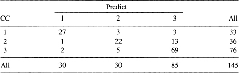
Table 12.10 Classification Table of Diabetes Data Using Multinomial Logistic Regression
Although we have taken 3 as the base level, from our computation we can derive other comparisons. We can get Logit (1/2) from the relation
We can judge how well the multinomial logistic regression classifies the observations into different categories. The methodology is similar to binary logistic regression. An observation is classified to that category for which it has the highest estimated probability. The classification table for the multinomial logistic regression is given in Table 12.10.
One can see that 118 out of 145 subjects studied are classified correctly by this procedure. 81% of the observations are correctly classified which is considerably higher than the maximum correct rate 59% (85/145), which would have been obtained if all the observations were put in one category. Multinomial logistic regression has performed well on this data. It is a powerful technique that should be used more extensively.
12.8.3 Ordered Response Category: Ordinal Logistic Regression
The response variable in many studies, as has been pointed out earlier, can be qualitative and fall in more than two categories. The categories may sometimes be ordered. In a consumer satisfaction study, the responses might be, highly satisfied, satisfied, dissatisfied, and highly dissatisfied. An analyst may want to study the socioeconomic and demographic factors that influence the response. The logistic model, slightly modified can be used for this analysis. The logits here are based on the cumulative probabilities. Several logistic models can be based on the cumulative logits. We describe one of these, the proportional odds model.
Again, we have n independent observations with p predictors. The response variable falls into k categories (1, 2,…, k). The k categories are ordered. Let Y denote the response variable. The cumulative distribution for Y is
![]()
Table 12.11 Ordinal Logistic Regression Model (Proportional Odds) Using SSPG and IR

The proportional odds model is given by,
![]()
for j = 1, 2,…, (k − 1). The comulative logit has a simple interpretation. It can be interpreted as the logit for a binary response in which the categories from 1 to j is one category, and the remaining categories from (j + 1) to k is the second category. The model is fitted by the maximum likelihood method. Several statistical software packages will carry out this procedure. Increase in the value of a response variable with a positive β will increase the probability of being in a lower numbered category, all other variables remaining the same. The number of parameters estimated to describe the data is fewer in the ordinal than in the nominal model. For a more detailed discussion the reader is referred to Agresti (2002) and Simonoff (2003).
12.8.4 Example: Determining Chemical Diabetes Revisited
We will use the data on chemical diabetes considered in Section 12.8.2 to illustrate ordinal logistic regression. The clinical classifications in the previous categories are ordered but we did not take it into consideration in our analysis. The progression of diabetes goes from normal (3), chemical (2), to overt diabetes (1). The classification states have a natural order and we will use them in our analysis. We will fit the proportional odds logit model. The result of the fit is given in Table 12.11.
The fit for the model is good. Both variables have significant relationship to the group membership. The coefficient of SSPG is positive. This indicates that higher values of SSPG increase the probability of being in a lower numbered category other factors being the same. The coefficient of IR is negative, indicating that higher values of this variable increase the probability of being in a higher numbered category, other factors remaining the same. The coefficient of concordance is high (0.90) showing the ability of the model to classify the group membership is high. In Table 12.12, we give the classification table for the ordinal logistic regression.
Table 12.12 Classification Table of Diabetes Data Using Multinomial Logistic Regression
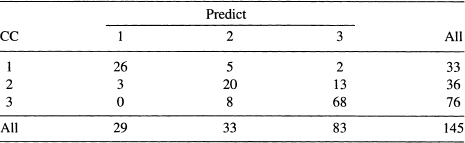
Of the 145 subjects ordinal logit regression classifies 114 subjects to their correct group. This gives the correct classification rate as 79%. This is comparable to the rate achieved by the multinomial logit model. It is generally expected that the ordinal model will do better than the multinomial model because of the additional information provided by the ordering of the categories. It should be also noted the ordinal logit model uses fewer parameters than the multinomial model. In our example the ordinal model uses 4 parameters, while the nominal version uses 6. For a more detailed discussion the reader is referred to Agresti (2002) and Simonoff (2003).
12.9 CLASSIFICATION PROBLEM: ANOTHER APPROACH
The method of logistic regression has been used to model the probability that an observation belongs to one group given the measurements on several characteristics. We have described how the fitted logits could then be used for classifying an observation into one of two categories. A different statistical methodology is available if our primary interest is classification. When the sole interest is to predict the group membership of each observation a statistical method called discriminant analysis is commonly used. Without discussing discriminant analysis here, we indicate a simple regression method that will accomplish the same task. The reader can find a discussion of discriminant analysis in McLachlan (1992), Rencher (1995), and Johnson (1998).
The essential idea in discriminant analysis is to find a linear combination of the predictor variables X1,…, Xp, such that the scores given by this linear combination separates the observations from the two groups as far as possible. One way that this separation can be accomplished is by fitting a multiple regression model to the data. The response variable is Y, taking values 0 and 1, and the predictors are X1,…, Xp. As has been pointed out earlier, some of the fitted values will be outside the range of 0 and 1. This does not matter here, as we are not trying to model probabilities, but only to predict group membership. We calculate the average of the predicted values of all the observations. If the predicted value for a given observation is greater than the average predicted value we assign that observation to the group which has Y = 1; if the predicted value is smaller than the average predicted value we assign it to the group with Y = 0. From this assignment we determine the number of observations classified correctly in the sample. The variables used in this classification procedure are determined exactly by the same methods as those used for variable selection in multiple regression.
Table 12.13 Results from the OLS Regression of Y on X1, X2, X3

We illustrate this method by applying it to the Bankruptcy data that we have used earlier to illustrate least squares regression. Table 12.13 gives the OLS regression results using the three predictor variables Xl, X2, and X3. All three variables have significant regression coefficients and should be retained for classification equation.
Table 12.14 displays the observed Y, the predicted Y, and the assigned group for the Bankruptcy data. The average value of the predicted Y is 0.5. All observations with predicted value less than 0.5 is assigned to Y = 0, and those with predicted value greater than 0.5 is assigned to the group with Y = 1. The wrongly classified observations are marked by *. It is seen that 5 bankrupt firms are classified as solvent, and one solvent firm is classified as bankrupt. The logistic regression, it should be noted, classified only two observations wrongly. One solvent firm and one bankrupt firm were misclassified. For the Bankruptcy data presented in Table 12.2, the logistic regression performs better than the multiple regression in classifying the sample data. In general this is true. The logistic regression does not have to make the restrictive assumption of multivariate normality for the predictor variables. For classification problems we recommend the use of logistic regression. If a logistic regression package is not available, then the multiple regression approach may be tried.
EXERCISES
12.1 The diagnostic plots in Figures 12.2, 12.3, and 12.4 show three unusual observations in the Bankruptcy data. Fit a logistic regression model to the 63 observations without these three observations and compare your results with the results obtained in Section 12.5. Does the deletion of the three points cause a substantial change in the logistic regression results?
Table 12.14 Classification of Observations by Fitted Values

12.2 Examine the various logistic regression diagnostics obtained from fitting the logistic regression Y on Xl and X2 (Table 12.3) and determine if the data contain unusual observations.
Table 12.15 Number of O-rings Damaged and the Temperature (Degrees Fahrenheit) at the Time of Launch for 23 Flights of the Space Shuttle Challenger

12.3 The O-rings in the booster rockets used in space launching play an important part in preventing rockets from exploding. Probabilities of O-ring failures are thought to be related to temperature. A detailed discussion of the background of the problem is found in The Flight of the Space Shuttle Challenger (pp. 33–35) in Chatterjee, Handcock, and Simonoff (1995). Each flight has six O-rings that could be potentially damaged in a particular flight. The data from 23 flights are given in Table 12.15 and can also be found in the the book's Web site.3 For each flight we have the number of O-rings damaged and the temperature of the launch.
(a) Fit a logistic regression connecting the probability of an O-ring failure with temperature. Interpret the coefficients.
(b) The data for Flight 18 that was launched when the launch temperature was 75 was thought to be problematic, and was deleted. Fit a logistic regression to the reduced data set. Interpret the coefficients.
(c) From the fitted model, find the probability of an O-ring failure when the temperature at launch was 31 degrees. This was the temperature forecast for the day of the launching of the fatal Challenger flight on January 20, 1986.
(d) Would you have advised the launching on that particular day?
12.4 Field-goal-kicking data for the entire American Football League (AFL) and National Football League (NFL) for the 1969 season are given in Table 12.16 and can also be found in the the book's Web site. Let π(X) denote the probability of kicking a field goal from a distance of X yards.
Table 12.16 Field-Goal-Kicking Performances of the American Football League (AFL) and National Football League (NFL) for the 1969 Season. The Variable Z Is an Indicator Variable Representing League

(a) For each of the leagues, fit the model
![]()
(b) Let Z be an indicator variable representing the league, that is,
![]()
Fit a single model combining the data from both leagues by extending the model to include the indicator variable Z that is, fit
![]()
(c) Does the quadratic term contribute significantly to the model?
(d) Are the probabilities of scoring field goals from a given distance the same for each league?
12.5 Using the data on diabetes analyzed in Tables 12.6 and 12.7, show that inclusion of the variable RW does not result in a substantial improvement in the classification rate from the multinomial logistic model using IR and SSPG.
12.6 Using the diabetes data in Tables 12.6 and 12.7, fit an ordinal logistic model using RW, IR, and SSPG to explain CC. Show that there is no substantial improvement in fit, and the correct classification rate from a model using only IR and SSPG.
1 See Chapter 6 for transformation of variables.