
CHAPTER 10
BIASED ESTIMATION OF REGRESSION COEFFICIENTS
10.1 INTRODUCTION
It was demonstrated in Chapter 9 that when multicollinearity is present in a set of predictor variables, the ordinary least squares estimates of the individual regression coefficients tend to be unstable and can lead to erroneous inferences. In this chapter, two alternative estimation methods that provide a more informative analysis of the data than the OLS method when multicollinearity is present are considered. The estimators discussed here are biased but tend to have more precision (as measured by mean square error) than the OLS estimators (see Draper and Smith (1998), McCallum (1970), and Hoerl and Kennard (1970)). These alternative methods do not reproduce the estimation data as well as the OLS method; the sum of squared residuals is not as small and, equivalently, the multiple correlation coefficient is not as large. However, the two alternatives have the potential to produce more precision in the estimated coefficients and smaller prediction errors when the predictions are generated using data other than those used for estimation.
Unfortunately, the criteria for deciding when these methods give better results than the OLS method depend on the true but unknown values of the model regression coefficients. That is, there is no completely objective way to decide when OLS should be replaced in favor of one of the alternatives. Nevertheless, when multicollinearity is suspected, the alternative methods of analysis are recommended. The resulting estimated regression coefficients may suggest a new interpretation of the data that, in turn, can lead to a better understanding of the process under study.
The two specific alternatives to OLS that are considered are (1) principal components regression and (2) ridge regression. Principal components analysis was introduced in Chapter 9. It is assumed that the reader is familiar with that material. It will be demonstrated that the principal components estimation method can be interpreted in two ways; one interpretation relates to the nonorthogonality of the predictor variables, the other has to do with constraints on the regression coefficients. Ridge regression also involves constraints on the coefficients. The ridge method is introduced in this chapter and it is applied again in Chapter 11 to the problem of variable selection. Both methods, principal components and ridge regression, are examined using the French import data that were analyzed in Chapter 9.
10.2 PRINCIPAL COMPONENTS REGRESSION
The model under consideration is
The variables are defined in Section 9.3. Let ![]() and
and ![]() be the means of Y and Xj, respectively. Also, let sy and sj be the standard deviations of Y and Xj respectively. The model of Equation (10.1) stated in terms of standardized variables (see Section 9.5) is
be the means of Y and Xj, respectively. Also, let sy and sj be the standard deviations of Y and Xj respectively. The model of Equation (10.1) stated in terms of standardized variables (see Section 9.5) is
where ![]() is the standardized version of the response variable and
is the standardized version of the response variable and ![]() is the standardized version of the jth predictor variable. Many regression packages produce values for both the regular and standardized regression coefficients in (10.1) and (10.2), respectively. The estimated coefficients satisfy
is the standardized version of the jth predictor variable. Many regression packages produce values for both the regular and standardized regression coefficients in (10.1) and (10.2), respectively. The estimated coefficients satisfy
The principal components of the standardized predictor variables are (see Equation (9.20))

These principal components were given in Table 9.13. The model in (10.2) may be written in terms of the principal components as
Table 10.1 Regression Results of Fitting Model (10.2) to the Import Data (1949–1959)

Table 10.2 Regression Results of Fitting Model (10.5) to the Import Data (1949–1959)

The equivalence of (10.2) and (10.5) follows since there is a unique relationship between the α's and θ's. In particular,

Conversely,

These same relationships hold for the least squares estimates, the ![]() and
and ![]() of the α's and θ's, respectively. Therefore, the
of the α's and θ's, respectively. Therefore, the ![]() and
and ![]() may be obtained by the regression of
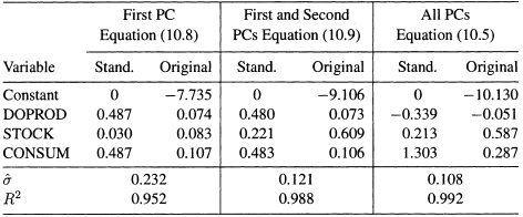
may be obtained by the regression of ![]() against the principal components C1, C2, and C3, or against the original standardized variables. The regression results of fitting models (10.2) and (10.5) to the import data are shown in Tables 10.1 and 10.2. From Table 10.1, the estimates of θ1, θ2, and θ3 are –0.339, 0.213, and 1.303, respectively. Similarly, from Table 10.2, the estimates of α1, α2, and α3 are 0.690, 0.191, and 1.160, respectively. The results in one of these tables can be obtained from the other table using (10.6) and (10.7).
against the principal components C1, C2, and C3, or against the original standardized variables. The regression results of fitting models (10.2) and (10.5) to the import data are shown in Tables 10.1 and 10.2. From Table 10.1, the estimates of θ1, θ2, and θ3 are –0.339, 0.213, and 1.303, respectively. Similarly, from Table 10.2, the estimates of α1, α2, and α3 are 0.690, 0.191, and 1.160, respectively. The results in one of these tables can be obtained from the other table using (10.6) and (10.7).
Although Equations (10.2) and (10.5) are equivalent, the C's in (10.5) are orthogonal. Observe, however, that the regression relationship given in terms of the principal components (Equation (10.5)) is not easily interpreted. The predictor variables of that model are linear combinations of the original predictor variables. The α's, unlike the θ's, do not have simple interpretations as marginal effects of the original predictor variables. Therefore, we use principal components regression only as a means for analyzing the multicollinearity problem. The final estimation results are always restated in terms of the θ's for interpretation.
10.3 REMOVING DEPENDENCE AMONG THE PREDICTORS
It has been mentioned that the principal components regression has two interpretations. We shall first use the principal components technique to reduce multi-collinearity in the estimation data. The reduction is accomplished by using less than the full set of principal components to explain the variation in the response variable. Note that when all three principal components are used, the OLS solution is reproduced exactly by applying Equations (10.7).
The C's have sample variances λ1 = 1.999, λ2 = 0.998, and λ3 = 0.003, respectively. Recall that the λ's are the eigenvalues of the correlation matrix of DOPROD, STOCK, and CONSUM. Since C3 has variance equal to 0.003, the linear function defining C3 is approximately equal to zero and is the source of multicollinearity in the data. We exclude C3 and consider regressions of ![]() against C1 alone as well as against C1 and C2. We consider the two possible regression models
against C1 alone as well as against C1 and C2. We consider the two possible regression models
and
Both models lead to estimates for all three of the original coefficients, θ1, θ2, and θ3. The estimates are biased since some information (C3 in Equation (10.9), C2 and C3 in Equation (10.8)) has been excluded in both cases.
The estimated values of α1 or α1 and α2 may be obtained by regressing ![]() in turn against C1 and then against C1 and C2. However, a simpler computational method is available that exploits the orthogonality of C1 C2 and C3.1 For example, the same estimated value of α1 will be obtained from regression using (10.5), (10.8), or (10.9). Similarly, the value of α2 may be obtained from (10.5) or (10.9). It also follows that if we have the OLS estimates of the θ's, estimates of the α's may be obtained from Equations (10.6). Then principal components regression estimates of the θ's corresponding to (10.8) and (10.9) can be computed by referring back to Equations (10.7) and setting the appropriate α's to zero. The following example clarifies the process.
in turn against C1 and then against C1 and C2. However, a simpler computational method is available that exploits the orthogonality of C1 C2 and C3.1 For example, the same estimated value of α1 will be obtained from regression using (10.5), (10.8), or (10.9). Similarly, the value of α2 may be obtained from (10.5) or (10.9). It also follows that if we have the OLS estimates of the θ's, estimates of the α's may be obtained from Equations (10.6). Then principal components regression estimates of the θ's corresponding to (10.8) and (10.9) can be computed by referring back to Equations (10.7) and setting the appropriate α's to zero. The following example clarifies the process.
Using α1 = 0.690 and α2 = α3 = 0 in Equations (10.7) yields estimated θ's corresponding to regression on only the first principal component, that is,
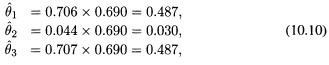
which yields
![]()
The estimates using the first two principal components, as in (10.9), are obtained in a similar fashion using α1 = 0.690, α2 =0.191, and α3= 0 in (10.7). The estimated of the regression coefficients, β0, β1, β2, and β3, of the original variables in Equation (10.1), can be obtained by substituting θ1, θ2, and θ3 in (10.3).
The estimates of the standardized and original regression coefficients using the three principal components models are shown in Table 10.3. It is evident that using different numbers of principal components gives substantially different results. It has already been argued that the OLS estimates are unsatisfactory. The negative coefficient of ![]() (DOPROD) is unexpected and cannot be sensibly interpreted. Furthermore, there is extensive multicollinearity which enters through the principal component, C3. This variable has almost zero variance (λ3 = 0.003) and is therefore approximately equal to zero. Of the two remaining principal components, it is fairly clear that the first one is associated with the combined effect of DOPROD and CONSUM. The second principal component is uniquely associated with STOCK. This conclusion is apparent in Table 10.3. The coefficients of DOPROD and CONSUM are completely determined from the regression of IMPORT on C1 alone. These coefficients do not change when C2 is used. The addition of C2 causes the coefficient of STOCK to increase from 0.083 to 0.609. Also, R2 increases from 0.952 to 0.988. Selecting the model based on the first two principal components, the resulting equation stated in original units is
(DOPROD) is unexpected and cannot be sensibly interpreted. Furthermore, there is extensive multicollinearity which enters through the principal component, C3. This variable has almost zero variance (λ3 = 0.003) and is therefore approximately equal to zero. Of the two remaining principal components, it is fairly clear that the first one is associated with the combined effect of DOPROD and CONSUM. The second principal component is uniquely associated with STOCK. This conclusion is apparent in Table 10.3. The coefficients of DOPROD and CONSUM are completely determined from the regression of IMPORT on C1 alone. These coefficients do not change when C2 is used. The addition of C2 causes the coefficient of STOCK to increase from 0.083 to 0.609. Also, R2 increases from 0.952 to 0.988. Selecting the model based on the first two principal components, the resulting equation stated in original units is
It provides a different and more plausible representation of the IMPORT relationship than was obtained from the OLS results. In addition, the analysis has led to an explicit quantification (in standardized variables) of the linear dependency in the predictor variables. We have C3 = 0 or equivalently (from Equations (10.4))
![]()
The standardized values of DOPROD and CONSUM are essentially equal. This information can be useful qualitatively and quantitatively if Equation (10.11) is used for forecasting or for analyzing policy decisions.
Table 10.3 Estimated Regression Coefficients for the Standardized and Original Variables Using Different Numbers of Principal Components for IMPORT Data (1949–1959)
10.4 CONSTRAINTS ON THE REGRESSION COEFFICIENTS
There is a second interpretation of the results of the principal components regression equation. The interpretation is linked to the notion of imposing constraints on the θ's which was introduced in Chapter 9. The estimates for Equation (10.9) were obtained by setting α3 equal to zero in Equations (10.7). From (10.6), α3 = 0 implies that
or ![]() . In original units, Equation (10.12) becomes
. In original units, Equation (10.12) becomes
or β1 = 0.69β3. Therefore, the estimates obtained by regression on C1 and C2 could have been obtained using OLS as in Chapter 9 with a linear constraint on the coefficients given by Equation (10.13).
Recall that in Chapter 9 we conjectured that β1 = β3 as a prior constraint on the coefficients. It was argued that the constraint was the result of a qualitative judgment based on knowledge of the process under study. It was imposed without looking at the data. Now, using the data, we have found that principal components regression on C1 and C2 gives a result that is equivalent to imposing the constraint of Equation (10.13). The result suggests that the marginal effect of domestic production on imports is about 69% of the marginal effect of domestic consumption on imports.
To summarize, the method of principal components regression provides both alternative estimates of the regression coefficients as well as other useful information about the underlying process that is generating the data. The structure of linear dependence among the predictor variables is made explicit. Principal components with small variances (eigenvalues) exhibit the linear relationships among the original variables that are the source of multicollinearity. Also elimination of multicollinearity by dropping one or more principal components from the regression is equivalent to imposing constraints on the regression coefficients. It provides a constructive way of identifying those constraints that are consistent with the proposed model and the information contained in the data.
10.5 PRINCIPAL COMPONENTS REGRESSION: A CAUTION
We have seen in Chapter 9 that principal components analysis is an effective tool for the detection of multicollinearity. In this chapter we have used the principal components as an alternative to the least squares method to obtain estimates of the regression coefficients in the presence of multicollinearity. The method has worked to our advantage in the Import data, where the first two of the three principal components have succeeded in capturing most of the variability in the response variable (see Table 10.3). This analysis is not guaranteed to work for all data sets. In fact, the principal components regression can fail in accounting for the variability in the response variable. To illustrate this point Hadi and Ling (1998) use a data set known as the Hald's data and a constructed response variable U. The original data set can be found in Draper and Smith (1998), p. 348. It is given here in Table and can also be found in the book's Web site.2 The data set has four predictor variables. The response variable U and the four PCs, C1,…, C4, corresponding to the four predictor variables are given in Table 10.5. The variable U is already in a standardized form, The sample variances of the four PCs are λ1 = 2.2357, λ2 = 1.5761, λ3 = 0.1866, and λ4 = 0.0016. The condition number, ![]()
![]() , is large, indicating the presence of multicollinearity in the original data.
, is large, indicating the presence of multicollinearity in the original data.
The regression results obtained from fitting the model
to the data are shown in Table 10.6. The coefficient of the last PC, C4, is highly significant and all other three coefficients are not significant. Now if we drop C4, the PC with the smallest variance, we obtain the results in Table 10.7. As it is clear from a comparison of Tables 10.6 and 10.7, all four PCs capture almost all the variability in U, while the first three account for none of the variability in U. Therefore, one should be careful before dropping any of the PCs.
Another problem with the principal component regression is that the results can be unduly influenced by the presence of high leverage point and outliers (see Chapter 4 for detailed discussion of outliers and influence). This is because the PCs are computed from the correlation matrix, which itself can be seriously affected by outliers in the data. A scatter plot of the response variable versus each of the PCs and the pairwise scatter plots of the PCs versus each other would point out outliers if they are present in the data. The scatter plot of U versus each of the PCs (Figure 10.1) show that there are no outliers in the data and U is related only to C4, which is consistent with the results in Tables 10.6 and 10.7. The pairwise scatter plots of the PCs versus each other (not shown) also show no outliers in the data. For other possible pitfalls of principal components regression see Hadi and Ling (1998).

Source: Draper and Smith (1998), p. 348
Table 10.5 A Response Variable U and a Set of Principal Components of Four Predictor Variables
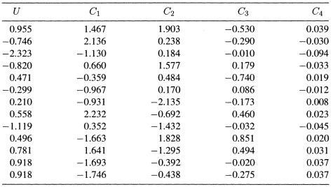
Table 10.6 Regression Results Using All Four PCs of Hald's Data
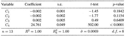
Table 10.7 Regression Results Using the First Three PCs of Hald's Data


Figure 10.1 Scatter plots of U versus each of the PCs of the Hald's data.
10.6 RIDGE REGRESSION
Ridge regression3 provides another alternative estimation method that may be used to advantage when the predictor variables are highly collinear. There are a number of alternative ways to define and compute ridge estimates (see the Appendix to this chapter). We have chosen to present the method associated with the ridge trace. It is a graphical approach and may be viewed as an exploratory technique. Ridge analysis using the ridge trace represents a unified approach to problems of detection and estimation when multicollinearity is suspected. The estimators produced are biased but tend to have a smaller mean squared error than OLS estimators (Hoerl and Kennard, 1970).
Ridge estimates of the regression coefficients may be obtained by solving a slightly altered form of the normal equations (introduced in Chapter 3). Assume that the standardized form of the regression model is given as:
The estimating equations for the ridge regression coefficients are

where rij is the correlation between the ith and jth predictor variables and riy is the correlation between the ith predictor variable and the response variable ![]() . The solution to (10.16),
. The solution to (10.16), ![]() , is the set of estimated ridge regression coefficients. The ridge estimates may be viewed as resulting from a set of data that has been slightly altered. See the Appendix to this chapter for a formal treatment.
, is the set of estimated ridge regression coefficients. The ridge estimates may be viewed as resulting from a set of data that has been slightly altered. See the Appendix to this chapter for a formal treatment.
The essential parameter that distinguishes ridge regression from OLS is k. Note that when k = 0, the ![]() 's are the OLS estimates. The parameter k may be referred to as the bias parameter. As k increases from zero, bias of the estimates increases. On the other hand, the total variance (the sum of the variances of the estimated regression coefficients), is
's are the OLS estimates. The parameter k may be referred to as the bias parameter. As k increases from zero, bias of the estimates increases. On the other hand, the total variance (the sum of the variances of the estimated regression coefficients), is
which is a decreasing function of k. The formula in (10.17) shows the effect of the ridge parameter on the total variance of the ridge estimates of the regression coefficients. Substituting k = 0 in (10.17), we obtain
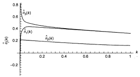
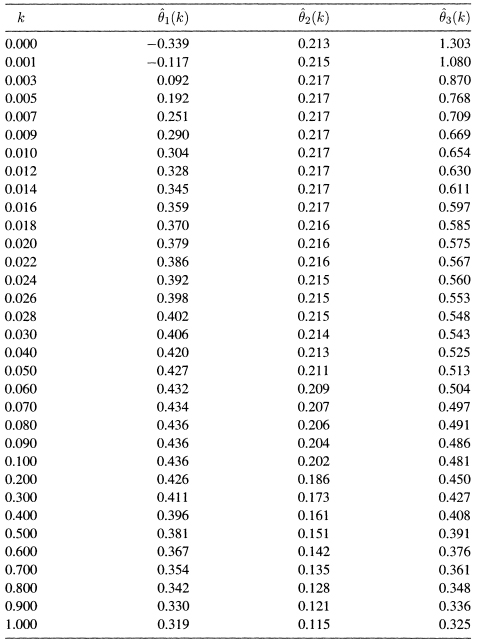
Figure 10.2 Ridge trace: IMPORT data (1949–1959).
which shows the effect of small eigenvalue on the total variance of the OLS estimates of the regression coefficients.
As k continues to increase without bound, the regression estimates all tend toward zero.4 The idea of ridge regression is to pick a value of k for which the reduction in total variance is not exceeded by the increase in bias.
It has been shown that there is a positive value of k for which the ridge estimates will be stable with respect to small changes in the estimation data (Hoerl and Kennard, 1970). In practice, a value of k is chosen by computing ![]() for a range of k values between 0 and 1 and plotting the results against k. The resulting graph is known as the ridge trace and is used to select an appropriate value for k. Guidelines for choosing k are given in the following example.
for a range of k values between 0 and 1 and plotting the results against k. The resulting graph is known as the ridge trace and is used to select an appropriate value for k. Guidelines for choosing k are given in the following example.
10.7 ESTIMATION BY THE RIDGE METHOD
A method for detecting multicollinearity that comes out of ridge analysis deals with the instability in the estimated coefficients resulting from slight changes in the estimation data. The instability may be observed in the ridge trace. The ridge trace is a simultaneous graph of the regression coefficients, ![]() , plotted against k for various values of k such as 0.001, 0.002, and so on. Figure 10.2 is the ridge. trace for the IMPORT data. The graph is constructed from Table 10.8, which has the ridge estimated coefficients for 29 values of k ranging from 0 to 1. Typically, the values of k are chosen to be concentrated near the low end of the range. If the estimated coefficients show large fluctuations for small values of k, instability has been demonstrated and multicollinearity is probably at work.
, plotted against k for various values of k such as 0.001, 0.002, and so on. Figure 10.2 is the ridge. trace for the IMPORT data. The graph is constructed from Table 10.8, which has the ridge estimated coefficients for 29 values of k ranging from 0 to 1. Typically, the values of k are chosen to be concentrated near the low end of the range. If the estimated coefficients show large fluctuations for small values of k, instability has been demonstrated and multicollinearity is probably at work.
What is evident from the trace or equivalently from Table 10.8 is that the estimated values of the coefficients θ1 and θ3 are quite unstable for small values of k. The estimate of θ1 changes rapidly from an implausible negative value of −0.339 to a stable value of about 0.43. The estimate of θ3 goes from 1.303 to stabilize at about 0.50. The coefficient of ![]() (STOCK), θ2 is unaffected by the multicollinearity and remains stable throughout at about 0.21.
(STOCK), θ2 is unaffected by the multicollinearity and remains stable throughout at about 0.21.
Table 10.8 Ridge Estimates ![]() , as Functions of the Ridge Parameter k, for the IMPORT Data (1949–1959)
, as Functions of the Ridge Parameter k, for the IMPORT Data (1949–1959)
The next step in the ridge analysis is to select a value of k and to obtain the corresponding estimates of the regression coefficients. If multicollinearity is a serious problem, the ridge estimators will vary dramatically as k is slowly increased from zero. As k increases, the coefficients will eventually stabilize. Since k is a bias parameter, it is desirable to select the smallest value of k for which stability occurs since the size of k is directly related to the amount of bias introduced. Several methods have been suggested for the choice of k. These methods include:
1. Fixed Point. Hoerl, Kennard, and Baldwin (1975) suggest estimating k by

where ![]() are the least squares estimates of θ1,…, θp when the model in (10.15) is fitted to the data (i.e., when k = 0), and
are the least squares estimates of θ1,…, θp when the model in (10.15) is fitted to the data (i.e., when k = 0), and ![]() is the corresponding residual mean square.
is the corresponding residual mean square.
2. Iterative Method. Hoerl and Kennard (1976) propose the following iterative procedure for selecting k: Start with the initial estimate of k in (10.19). Denote this value by k0. Then, calculate

Then use k1 to calculate k2 as

Repeat this process until the difference between two successive estimates of k is negligible.
3. Ridge Trace. The behavior of ![]() as a function of k is easily observed from the ridge trace. The value of k selected is the smallest value for which all the coefficients
as a function of k is easily observed from the ridge trace. The value of k selected is the smallest value for which all the coefficients ![]() are stable. In addition, at the selected value of k, the residual sum of squares should remain close to its minimum value. The variance inflation factors.5 VIFj(k), should also get down to less than 10. (Recall that a value of 1 is a characteristic of an orthogonal system and a value less than 10 would indicate a non-collinear or stable system.)
are stable. In addition, at the selected value of k, the residual sum of squares should remain close to its minimum value. The variance inflation factors.5 VIFj(k), should also get down to less than 10. (Recall that a value of 1 is a characteristic of an orthogonal system and a value less than 10 would indicate a non-collinear or stable system.)
4. Other Methods. Many other methods for estimating k have been suggested in the literature. See, for example, Marquardt (1970), Mallows (1973), Goldstein and Smith (1974), McDonald and Galarneau (1975), Dempster et al. (1977), and Wahba, Golub, and Health (1979). The appeal of the ridge trace, however, lies in its graphical representation of the effects that multicollinearity has on the estimated coefficients.
For the IMPORT data, the fixed point formula in (10.19) gives
The iterative method gives the following sequence: k0 = 0.0164, k1 = 0.0161, and k2 = 0.0161. So, it converges after two iterations to k = 0.0161. The ridge trace in Figure 10.2 (see also Table 10.8) appears to stabilize for k around 0.04. We therefore have three estimates of k (0.0164, 0.0161, and 0.04).
From Table 10.8, we see that at any of these values the improper negative sign on the estimate of θ1 has disappeared and the coefficient has stabilized (at 0.359 for k = 0.016 and at 0.42 for k = 0.04). From Table 10.9, we see that the sum of squared residuals (SSE(k)) has only increased from 0.081 at k = 0 to 0.108 at k = 0.016, and to 0.117 at k = 0.04. Also, the variance inflation factors, VIF1(k) and VIF3(k), decreased from about 185 to values between 1 and 4. It is clear that values of k in the interval (0.016 to 0.04) appear to be satisfactory.
The estimated coefficients from the model stated in standardized and original variables units are summarized in Table 10.10. The original coefficient ![]() is obtained from the standardized coefficient
is obtained from the standardized coefficient ![]() using (10.3). For example,
using (10.3). For example, ![]() calculated by
calculated by
![]()
Thus, the resulting model in terms for the original variables fitted by ridge method using k = 0.04 is
![]()
The equation gives a plausible representation of the relationship. Note that the final equation for these data is not particularly different from the result obtained by using the first two principal components (see Table 10.3), although the two computational methods appear to be very different.
10.8 RIDGE REGRESSION: SOME REMARKS
Ridge regression provides a tool for judging the stability of a given body of data for analysis by least squares. In highly collinear situations, as has been pointed out, small changes (perturbations) in the data cause very large changes in the estimated regression coefficients. Ridge regression will reveal this condition. Least squares regression should be used with caution in these situations. Ridge regression provides estimates that are more robust than least squares estimates for small perturbations in the data. The method will indicate the sensitivity (or the stability) of the least squares coefficients to small changes in the data.
Table 10.9 Residual Sum of Squares, SSE(k), and Variance Inflation Factors, VIFj(k), as Functions of the Ridge Parameter k, for the IMPORT Data (1949–1959)

Table 10.10 OLS and Ridge Estimates of the Regression Coefficients for IMPORT Data (1949–1959)

The ridge estimators are stable in the sense that they are not affected by slight variations in the estimation data. Because of the smaller mean square error property, values of the ridge estimated coefficients are expected to be closer than the OLS estimates to the true values of the regression coefficients. Also, forecasts of the response variable corresponding to values of the predictor variables not included in the estimation set tend to be more accurate.
The estimation of the bias parameter k is rather subjective. There are many methods for estimating k but there is no consensus as to which method is preferable. Regardless of the method of choice for estimating the ridge parameter k, the estimated parameter can be affected by the presence of outliers in the data. Therefore a careful checking for outliers should accompany any method for estimating k to ensure that the obtained estimate is not unduly influenced by outliers in the data.
As with the principal components method, the criteria for deciding when the ridge estimators are superior to the OLS estimators depend on the values of the true regression coefficients in the model. Although these values cannot be known, we still suggest that ridge analysis is useful in cases where extreme multicollinearity is suspected. The ridge coefficients can suggest an alternative interpretation of the data that may lead to a better understanding of the process under study.
Another practical problem with ridge regression is that it has not been implemented in some statistical packages. If a statistical package does not have a routine for ridge regression, ridge regression estimates can be obtained from the standard least squares package by using a slightly altered data set. Specifically, the ridge estimates of the regression coefficients can be obtained from the regression of Y* on ![]() . The new response variable Y* is obtained by augmenting
. The new response variable Y* is obtained by augmenting ![]() by p new fictitious observations, each of which is equal to zero. Similarly, the new predictor variable
by p new fictitious observations, each of which is equal to zero. Similarly, the new predictor variable ![]() is obtained by augmenting
is obtained by augmenting ![]() by p new fictitious observations, each of which is equal to zero except the one in the jth position which is equal to
by p new fictitious observations, each of which is equal to zero except the one in the jth position which is equal to ![]() , where k is the chosen value of the ridge parameter. It can be shown that the ridge estimates
, where k is the chosen value of the ridge parameter. It can be shown that the ridge estimates ![]() are obtained by the least squares regression of Y* on
are obtained by the least squares regression of Y* on ![]() without having a constant term in the model.
without having a constant term in the model.
10.9 SUMMARY
Both alternative estimation methods, ridge regression and principal components regression, provide additional information about the data being analyzed. We have seen that the eigenvalues of the correlation matrix of predictor variables play an important role in detecting multicollinearity and in analyzing its effects. The regression estimates produced by these methods are biased but may be more accurate than OLS estimates in terms of mean square error. It is impossible to evaluate the gain in accuracy for a specific problem since a comparison of the two methods to OLS requires knowledge of the true values of the coefficients. Nevertheless, when severe multicollinearity is suspected, we recommend that at least one set of estimates in addition to the OLS estimates be calculated. The estimates may suggest an interpretation of the data that were not previously considered.
There is no strong theoretical justification for using principal components or ridge regression methods. We recommend that the methods be used in the presence of severe multicollinearity as a visual diagnostic tool for judging the suitability of the data for least squares analysis. When principal components or ridge regression analysis reveal the instability of a particular data set, the analyst should first consider using least squares regression on a reduced set of variables (as indicated in Chapter 9). If least squares regression is still unsatisfactory (high VIFs, coefficients with wrong signs, large condition number), only then should principal components or ridge regression be used.
EXERCISES
10.1 Longley's (1967) data set is a classic example of multicollinear data. The data (Table 10.11) consist of a response variable S and six predictor variables X1,…, X6. The data can be found in the book's Web site. The initial model
in terms of the original variables, can be written in terms of the standardized variables as
(a) Fit the model (10.24) to the data using least squares. What conclusion can you draw from the data?
(b) From the results you obtained from the model in (10.24), obtain the least squares estimated regression coefficients in model (10.23).
Table 10.11 Longley (1967) Data

(c) Now fit the model in (10.23) to the data using least squares and verify that the obtained results are consistent with those obtained above.
(d) Compute the correlation matrix of the six predictor variables and the corresponding scatter plot matrix. Do you see any evidence of collinearity?
(e) Compute the corresponding PCs, their sample variances, and the condition number. How many different sets of multicollinearity exist in the data? What are the variables involved in each set?
(f) Based on the number of PCs you choose to retain, obtain the PC estimates of the coefficients in (10.23) and (10.24).
(g) Using the ridge method, construct the ridge trace. What value of k do you recommend to be used in the estimation of the parameters in (10.23) and (10.24)? Use the chosen value of k and compute the ridge estimates of the regression coefficients in (10.23) and (10.24).
(h) Compare the estimates you obtained by the three methods. Which one would you recommend? Explain.
10.2 Repeat Exercise 10.1 using the Hald's data discussed in Section 10.5 but using the original response variable Y and the four predictors X1,…, X4. The data appear in Table 10.4.
10.3 From your analysis of the Longley and Hald data sets, do you observe the sort of problems pointed out in Section 10.5?
Appendix: Ridge Regression
In this appendix we present ridge regression method in matrix notation.
A. The Model
The regression model can be expressed as
where Y is an n × 1 vector of observations on the response variable, Z = (Z1,…, Zp) is an n × p matrix of n observations on p predictor variables, θ is a p × 1 vector of regression coefficients, and ε is an n × 1 vector of random errors. It is assumed that E(ε) = 0, E(εεT) = σ2I, where I is the identity matrix of order n. It is also assumed, without loss of generality, that Y and Z have been centered and scaled so that ZTZ and ZTY are matrices of correlation coefficients.6
The least squares estimator for θ is ![]() . It can be shown that
. It can be shown that
where λ1 ≥ λ2 ≥ … ≥ λp are the eigenvalues of ZTZ. The left-hand side of (A.2) is called the total mean square error. It serves as a composite measure of the squared distance of the estimated regression coefficients from their true values.
B. Effect of Multicollinearity
It was argued in Chapter 9 and in the Appendix to Chapter 9 that multi-collinearity is synonymous with small eigenvalues. It follows from Equation (A.2) that when one or more of the λ's are small, the total mean square error of ![]() is large, suggesting imprecision in the least squares estimation method. The ridge regression approach is an attempt to construct an alternative estimator that has a smaller total mean square error value.
is large, suggesting imprecision in the least squares estimation method. The ridge regression approach is an attempt to construct an alternative estimator that has a smaller total mean square error value.
C. Ridge Regression Estimators
Hoerl and Kennard (1970) suggest a class of estimators indexed by a parameter k > 0. The estimator is (for a given value of k)
The expected value of ![]() is
is
and the variance-covariance matrix is
The variance inflation factor, VIFj(k), as a function of k is the jth diagonal element of the matrix ![]() .
.
The residual sum of squares can be written as
The total mean square error is

Note that the first term on the right-hand side of Equation (A.7) is the sum of the variances of the components of ![]() (total variance) and the second term is the square of the bias. Hoerl and Kennard (1970) prove that there exists a value of k > 0 such that
(total variance) and the second term is the square of the bias. Hoerl and Kennard (1970) prove that there exists a value of k > 0 such that
![]()
that is, the mean square error of the ridge estimator, ![]() , is less than the mean square error of the OLS estimator,
, is less than the mean square error of the OLS estimator, ![]() . Hoerl and Kennard (1970) suggest that an appropriate value of k may be selected by observing the ridge trace and some complementary summary statistics for
. Hoerl and Kennard (1970) suggest that an appropriate value of k may be selected by observing the ridge trace and some complementary summary statistics for ![]() such as SSE(k) and VIFj(k). The value of k selected is the smallest value for which
such as SSE(k) and VIFj(k). The value of k selected is the smallest value for which ![]() is stable. In addition, at the selected value of k, the residual sum of squares should remain close to its minimum value, and the variance inflation factors are less than 10, as discussed in Chapter 9.
is stable. In addition, at the selected value of k, the residual sum of squares should remain close to its minimum value, and the variance inflation factors are less than 10, as discussed in Chapter 9.
Ridge estimators have been generalized in several ways. They are sometimes generically referred to as shrinkage estimators, because these procedures tend to shrink the estimates of the regression coefficients toward zero. To see one possible generalization, consider the regression model restated in terms of the principal components, C = (C1,…, Cp), discussed in the Appendix to Chapter 9. The general model takes the form
where

is a diagonal matrix consisting of the ordered eigenvalues of ZTZ. The total mean square error in (A.7) becomes

where αT = (α1, α2,…, αp). Instead of taking a single value for k, we can consider several different values k, say k1, k2,…, kp. We consider separate ridge parameters (i.e., shrinkage factors) for each of the regression coefficients. The quantity k, instead of being a scalar, is now a vector and denoted by k. The total mean square error given in (A. 10) now becomes

The total mean square error given in (A. 11) is minimized by taking ![]() . An iterative estimation procedure is suggested. At Step 1, kj is computed by using ordinary least squares estimates for σ2 and αj. Then a new value of
. An iterative estimation procedure is suggested. At Step 1, kj is computed by using ordinary least squares estimates for σ2 and αj. Then a new value of ![]() (k) is computed,
(k) is computed,
![]()
where K is a diagonal matrix with diagonal elements k1,…, kp from Step 1. The process is repeated until successive changes in the components of ![]() (k) are negligible. Then, using Equation (A.9), the estimate of θ is
(k) are negligible. Then, using Equation (A.9), the estimate of θ is
The two ridge-type estimators (one value of k, several values of k) defined previously, as well as other related alternatives to ordinary least-squares estimation, are discussed by Dempster et al. (1977). The different estimators are compared and evaluated by Monte Carlo techniques. In general, the choice of the best estimation method for a particular problem depends on the specific model and data. Dempster et al. (1977) hint at an analysis that could be used to identify the best estimation method for a given set of data. At the present time, our preference is for the simplest version of the ridge method, a single ridge parameter k, chosen after an examination of the ridge trace.
1 In any regression equation where the full set of potential predictor variables under consideration are orthogonal, the estimated values of regression coefficients are not altered when subsets of these variables are either introduced or deleted.
2 http://www.ilr.cornell.edu/˜hadi/RABE4.
3 Hoerl (1959) named the method ridge regression because of its similarity to ridge analysis used in his earlier work to study second-order response surfaces in many variables.
4 Because the ridge method tends to shrink the estimates of the regression coefficients toward zero, ridge estimators are sometimes generically referred to as shrinkage estimators.
5 The formula for VIFj(k) is given in the Appendix to this chapter.
6 Note that Zj is obtained by transforming the original predictor variable Xj by zij = (xij − ![]() . Thus, Zj is centered and scaled to have unit length, that is,
. Thus, Zj is centered and scaled to have unit length, that is, ![]() .
.