CHAPTER 5

QUALITATIVE VARIABLES AS PREDICTORS

5.1 INTRODUCTION

Qualitative or categorical variables can be very useful as predictor variables in regression analysis. Qualitative variables such as sex, marital status, or political affiliation can be represented by indicator or dummy variables. These variables take on only two values, usually 0 and 1. The two values signify that the observation belongs to one of two possible categories. The numerical values of indicator variables are not intended to reflect a quantitative ordering of the categories, but only serve to identify category or class membership. For example, an analysis of salaries earned by computer programmers may include variables such as education, years of experience, and sex as predictor variables. The sex variable could be quantified, say, as 1 for female and 0 for male. Indicator variables can also be used in a regression equation to distinguish among three or more groups as well as among classifications across various types of groups. For example, the regression described above may also include an indicator variable to distinguish whether the observation was for a systems or applications programmer. The four conditions determined by sex and type of programming can be represented by combining the two variables, as we shall see in this chapter.

Table 5.1 Salary Survey Data

Indicator variables can be used in a variety of ways and may be considered whenever there are qualitative variables affecting a relationship. We shall illustrate some of the applications with examples and suggest some additional applications. It is hoped that the reader will recognize the general applicability of the technique from the examples. In the first example, we look at data on a salary survey, such as the one mentioned above, and use indicator variables to adjust for various categorical variables that affect the regression relationship. The second example uses indicator variables for analyzing and testing for equality of regression relationships in various subsets of a population.

We continue to assume that the response variable is a quantitative continuous variable, but the predictor variables can be quantitative and/or categorical. The case where the response variable is an indicator variable is dealt with in Chapter 12.

5.2 SALARY SURVEY DATA

The Salary Survey data set was developed from a salary survey of computer professionals in a large corporation. The objective of the survey was to identify and quantify those variables that determine salary differentials. In addition, the data could be used to determine if the corporation's salary administration guidelines were being followed. The data appear in Table 5.1 and can be obtained from the book's Web site.¹ The response variable is salary (S) and the predictors are: (1) experience (X), measured in years; (2) education (E), coded as 1 for completion of a high school (H.S.) diploma, 2 for completion of a bachelor degree (B.S.), and 3 for the completion of an advanced degree; and (3) management (M), which is coded as 1 for a person with management responsibility and 0 otherwise. We shall try to measure the effects of these three variables on salary using regression analysis.

A linear relationship will be used for salary and experience. We shall assume that each additional year of experience is worth a fixed salary increment. Education may also be treated in a linear fashion. If the education variable is used in the regression equation in raw form, we would be assuming that each step up in education is worth a fixed increment to salary. That is, with all other variables held constant, the relationship between salary and education is linear. That interpretation is possible but may be too restrictive. Instead, we shall view education as a categorical variable and define two indicator variables to represent the three categories. These two variables allow us to pick up the effect of education on salary whether or not it is linear. The management variable is also an indicator variable designating the two categories, 1 for management positions and 0 for regular staff positions.

Note that when using indicator variables to represent a set of categories, the number of these variables required is one less than the number of categories. For example, in the case of the education categories above, we create two indicator variables E₁ and E₂, where

and

As stated above, these two variables taken together uniquely represent the three groups. For H.S., E₁ = 1, E₂ = 0; for B.S., E₁ = 0, E₂ = 1; and for advanced degree, E₁ = 0, E₂ = 0. Furthermore, if there were a third variable, E_i3, defined to be 1 or 0 depending on whether or not the ith person is in the advanced degree category, then for each person we have E₁ + E₂ + E₃ = 1. Then E₃ = 1 − E₁ − E₂, showing clearly that one of the variables is superfluous.² Similarly, there is only one indicator variable required to distinguish the two management categories. The category that is not represented by an indicator variable is referred to as the base category or the control group because the regression coefficients of the indicator variables are interpreted relative to the control group.

Table 5.2 Regression Equationsfor the Six Categories of Educationand Management

Table 5.3 Regression Analysisof Salary Survey Data

In terms of the indicator variables described above, the regression model is

By evaluating (5.1) for the different values of the indicator variables, it follows that there is a different regression equation for each of the six (three education and two management) categories as shown in Table 5.2. According to the proposed model, we may say that the indicator variables help to determine the base salary level as a function of education and management status after adjustment for years of experience.

The results of the regression computations for the model given in (5.1) appear in Table 5.3. The proportion of salary variation accounted for by the model is quite high (R² = 0.957). At this point in the analysis we should investigate the pattern of residuals to check on model specification. We shall postpone that investigation for now and assume that the model is satisfactory so that we can discuss the interpretation of the regression results. Later we shall return to analyze the residuals and find that the model must be altered.

We see that the coefficient of X is 546.16. That is, each additional year of experience is estimated to be worth an annual salary increment of $546. The other coefficients may be interpreted by looking into Table 5.2. The coefficient of the management indicator variable, δ₁, is estimated to be 6883.50. From Table 5.2 we interpret this amount to be the average incremental value in annual salary associated with a management position. For the education variables, γ₁ measures the salary differential for the H.S. category relative to the advanced degree category and γ₂ measures the differential for the B.S. category relative to the advanced degree category. The difference, γ₂ − γ₁, measures the differential salary for the H.S. category relative to the B.S. category. From the regression results, in terms of salary for computer professionals, we see that an advanced degree is worth $2996 more than a high school diploma, a B.S. is worth $148 more than an advanced degree (this differential is not statistically significant, t = 0.38), and a B.S. is worth about $3144 more than a high school diploma. These salary differentials hold for every fixed level of experience.

5.3 INTERACTION VARIABLES

Returning now to the question of model specification, consider Figure 5.1, where the residuals are plotted against X. The plot suggests that there may be three or more specific levels of residuals. Possibly the indicator variables that have been defined are not adequate for explaining the effects of education and management status. Actually, each residual is identified with one of the six education-management combinations. To see this we plot the residuals against Category (a new categorical variable that takes a separate value for each of the six combinations). This graph is, in effect, a plot of residuals versus a potential predictor variable that has not yet been used in the equation. The graph is given in Figure 5.2. It can be seen from the graph that the residuals cluster by size according to their education-management category. The combinations of education and management have not been satisfactorily treated in the model. Within each of the six groups, the residuals are either almost totally positive or totally negative. This behavior implies that the model given in (5.1) does not adequately explain the relationship between salary and experience, education, and management variables. The graph points to some hidden structure in the data that has not been explored.

The graphs strongly suggest that the effects of education and management status on salary determination are not additive. Note that in the model in (5.1) and its further exposition in Table 5.2, the incremental effects of both variables are determined by additive constants. For example, the effect of a management position is measured as δ₁, independently of the level of educational attainment. The nonadditive effects of these variables can be evaluated by constructing additional variables that are used to measure what may be referred to as multiplicative or interaction effects. Interaction variables are defined as products of the existing indicator variables (E₁ · M) and (E₂ · M). The inclusion of these two variables on the right-hand side of (5.1) leads to a model that is no longer additive in education and management, but recognizes the multiplicative effect of these two variables.

Figure 5.1 Standardized residuals versus years of experience (X).

Figure 5.2 Standardized residuals versus education-management categorical variable.

Table 5.4 Regression Analysis of Salary Data: Expanded Model

Table 5.5 Regression Analysis of Salary Data: Expanded Model, Observation 33 Deleted.

The expanded model is

The regression results are given in Table 5.4. The residuals from the regression of the expanded model are plotted against X in Figure 5.3. Note that observation 33 is an outlier. Salary is overpredicted by the model. Checking this observation in the listing of the raw data, it appears that this particular person seems to have fallen behind by a couple of hundred dollars in annual salary as compared to other persons with similar characteristics. To be sure that this single observation is not overly affecting the regression estimates, it has been deleted and the regression rerun. The new results are given in Table 5.5.

The regression coefficients are basically unchanged. However, the standard deviation of the residuals has been reduced to $67.28 and the proportion of explained variation has reached 0.9998. The plot of residuals versus X (Figure 5.4) appears to be satisfactory compared with the similar residual plot for the additive model. In addition, the plot of residuals for each education-management category (Figure 5.5) shows that each of these groups has residuals that appear to be symmetrically distributed about zero. Therefore the introduction of the interaction terms has produced an accurate representation of salary variations. The relationships between salary and experience, education, and management status appear to be adequately described by the model given in (5.2).

With the standard error of the residuals estimated to be $67.28, we can believe that we have uncovered the actual and very carefully administered salary formula. Using 95% confidence intervals, each year of experience is estimated to be worth between $494.08 and $502.72. These increments of approximately $500 are added to a starting salary that is specified for each of the six education-management groups. Since the final regression model is not additive, it is rather difficult to directly interpret the coefficients of the indicator variables. To see how the qualitative variables affect salary differentials, we use the coefficients to form estimates of the base salary for each of the six categories. These results are presented in Table 5.6 along with standard errors and confidence intervals. The standard errors are computed using Equation (A.12) in the Appendix to Chapter 3.

Using a regression model with indicator variables and interaction terms, it has been possible to account for almost all the variation in salaries of computer professionals selected for this survey. The level of accuracy with which the model explains the data is very rare! We can only conjecture that the methods of salary administration in this company are precisely defined and strictly applied.

In retrospect, we see that an equivalent model may be obtained with a different set of indicator variables and regression parameters. One could define five variables, each taking on the values of 1 or 0, corresponding to five of the six education-management categories. The numerical estimates of base salary and the standard errors of Table 5.6 would be the same. The advantage to proceeding as we have is that it allows us to separate the effects of the three sets of predictor variables, (1) education, (2) management, and (3) education-management interaction. Recall that interaction terms were included only after we found that an additive model did not satisfactorily explain salary variations. In general, we start with simple models and proceed sequentially to more complex models if necessary. We shall always hope to retain the simplest model that has an acceptable residual structure.

5.4 SYSTEMS OF REGRESSION EQUATIONS: COMPARING TWO GROUPS

A collection of data may consist of two or more distinct subsets, each of which may require a separate regression equation. Serious bias may be incurred if one regression relationship is used to represent the pooled data set. An analysis of this problem can be accomplished using indicator variables. An analysis of separate regression equations for subsets of the data may be applied to cross-sectional or time series data. The example discussed below treats cross-sectional data. Applications to time series data are discussed in Section 5.5.

Figure 5.3 Standardized residuals versus years of experience: Expanded model.

Figure 5.4 Standardized residuals versus years of experience: Expanded model, observation 33 deleted.

Figure 5.5 Standardized residuals versus education-management categorical variable: Expanded model, observation 33 deleted.

Table 5.6 Estimates of Base Salary Using the Nonadditive Model in (5.2)

The model for the two groups can be different in all aspects or in only some aspects. In this section we discuss three distinct cases:

1. Each group has a separate regression model.
2. The models have the same intercept but different slopes.
3. The models have the same slope but different intercepts.

We illustrate these cases below when we have only one quantitative predictor variable. These ideas can be extended straightforwardly to the cases where there are more than one quantitative predictor variable.

5.4.1 Models with Different Slopes and Different Intercepts

We illustrate this case with an important problem concerning equal opportunity in employment. Many large corporations and government agencies administer a preemployment test in an attempt to screen job applicants. The test is supposed to measure an applicant's aptitude for the job and the results are used as part of the information for making a hiring decision. The federal government has ruled³ that these tests (1) must measure abilities that are directly related to the job under consideration and (2) must not discriminate on the basis of race or national origin. Operational definitions of requirements (1) and (2) are rather elusive. We shall not try to resolve these operational problems. We shall take one approach involving race represented as two groups, white and minority. The hypothesis that there are separate regressions relating test scores to job performance for the two groups will be examined. The implications of this hypothesis for discrimination in hiring are discussed.

Figure 5.6 Requirements for employment on pretest.

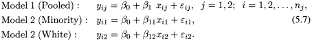
Let Y represent job performance and let X be the score on the preemployment test. We want to compare

Figure 5.6 depicts the two models. In model 1, race distinction is ignored, the data are pooled, and there is one regression line. In model 2 there is a separate regression relationship for the two subgroups, each with distinct regression coefficients. We shall assume that the variances of the residual terms are the same in each subgroup.

Before analyzing the data, let us briefly consider the types of errors that could be present in interpreting and applying the results. If Y₀, as seen on the graph, has been set as the minimum required level of performance, then using Model 1, an acceptable score on the test is one that exceeds X_p. However, if Model 2 is in fact correct, the appropriate testscore for whites is X_w and for minorities is X_m. Using X_p in place of X_m and X_w represents a relaxation of the pretest requirement for whites and a tightening of that requirement for minorities. Since inequity can result in the selection procedure if the wrong model is used to set cutoff values, it is necessary to examine the data carefully. It must be determined whether there are two distinct relationships or whether the relationship is the same for both groups and a single equation estimated from the pooled data is adequate. Note that whether Modell or Model 2 is chosen, the values X_m, X_w, and X_p are estimates subject to sampling errors and should only be used in conjunction with appropriate confidence intervals. (Construction of confidence intervals is discussed in the following paragraphs.)

Data were collected for this analysis using a special employment program. Twenty applicants were hired on a trial basis for six weeks. One week was spent in a training class. The remaining five weeks were spent on the job. The participants were selected from a pool of applicants by a method that was not related to the preemployment test scores. A test was given at the end of the training period and a work performance evaluation was developed at the end of the six-week period.

Table 5.7 Data on Preemployment Testing Program

These two scores were combined to form an index of job performance. (Those employees with unsatisfactory performance at the end of the six-week period were dropped.) The data appear in Table 5.7 and can be obtained from the book's Web site. We refer to this data set as the Preemployment Testing data.

Formally, we want to test the null hypothesis H₀, : β₁₁ = β₁₂, β₀₁ = β₀₂ against the alternative that there are substantial differences in these parameters. The test can be performed using indicator variables. Let z_ij be defined to take the value 1 if j = 1 and to take the value 0 if j = 2. That is, Z is a new variable that has the value 1 for a minority applicant and the value 0 for a white applicant. We consider the two models,

The variable (z_ij · x_ij) represents the interaction between the group (race) variable, Z and the preemployment test X. Note that Model 3 is equivalent to Model 2. This can be seen if we observe that for the minority group, x_ij = x_i1 and z_ij = l; hence Model 3 becomes

which is the same as Model 2 for minority with β₀₁ = β₀ + γ and β₁₁ = β₁ + δ. Similarly, for the white group, we have x_ij = x_i2, z_ij = 0, and Model 3 becomes

which is the same as Model 2 for white with β₀₂ = β₀ and β₁₂ = β₁. Therefore, a comparison between Models 1 and 2 is equivalent to a comparison between Models 1 and 3. Note that Model 3 can be viewed as a full model (FM) and Model 1 as a restricted model (RM) because Model 1 is obtained from Model 3 by setting γ = δ = 0. Thus, our null hypothesis H₀ now becomes H₀ : γ = δ = 0. The hypothesis is tested by constructing an F-test for the comparison of two models as described in Chapter 3. In this case, the test statistics is

Table 5.8 Regression Results, Preemployment Testing Data: Model 1

Table 5.9 Regression Results, Preemployment Testing Data: Model 3

which has 2 and 16 degrees of freedom. (Why?) Proceeding with the analysis of the data, the regression results for Modell and Model 3 are given in Tables 5.8 and 5.9. The plots of residuals against the predictor variable (Figures 5.7 and 5.8) look acceptable in both cases. The one residual at the lower right in Model 1 may require further investigation.

To evaluate the formal hypothesis we compute the F -ratio specified previously, which is equal to

and is significant at a level slightly above 5%. Therefore, on the basis of this test we would conclude that the relationship is probably different for the two groups. Specifically, for minorities we have

and for whites we have

Figure 5.7 Standardized residuals versus test score: Model 1.

Figure 5.8 Standardized residuals versus test score: Model 3.

Figure 5.9 Standardized residuals versus race: Model 1.

Table 5.10 Separate Regression Results

The results are very similar to those that were described in Figure 5.5 when the problem of bias was discussed. The straight line representing the relationship for minorities has a larger slope and a smaller intercept than the line for whites. If a pooled model were used, the types of biases discussed in relation to Figure 5.6 would occur.

Although the formal procedure using indicator variables has led to the plausible conclusion that the relationships are different for the two groups, the data for the individual groups have not been looked at carefully. Recall that it was assumed that the variances were identical in the two groups. This assumption was required so that the only distinguishing characteristic between the two samples was the pair of regression coefficients. In Figure 5.9 a plot of residuals versus the indicator variable is presented. There does not appear to be a difference between the two sets of residuals. We shall now look more closely at each group. The regression coefficients for each sample taken separately are presented in Table 5.10. The residuals are shown in Figures 5.10 and 5.11. The regression coefficients are, of course, the values obtained from Model 3. The standard errors of the residuals are 1.29 and 1.51 for the minority and white samples, respectively. The residual plots against the test score are acceptable in both cases. An interesting observation that was not available in the earlier analysis is that the preemployment test accounts for a major portion of the variation in the minority sample, but the test is only marginally useful in the white sample.

Figure 5.10 Standardized residuals versus test: Model 1, minority only.

Figure 5.11 Standardized residuals versus test: Model 1, white only.

Our previous conclusion is still valid. The two regression equations are different. Not only are the regression coefficients different, but the residual mean squares also show slight differences. Of more importance, the values of R² are greatly different. For the white sample, R² = 0.29 is so small (t = 1.82; 2.306 is required for significance) that the preemployment test score is not deemed an adequate predictor of job success. This finding has bearing on our original objective since it should be a prerequisite for comparing regressions in two samples that the relationships be valid in each of the samples when taken alone. Concerning the validity of the preemployment test, we conclude that if applied as the law prescribes, with indifference to race, it will give biased results for both racial groups. Moreover, based on these findings, we may be justified in saying that the test is of no value for screening white applicants.

We close the discussion with a note about determining the appropriate cutoff test score if the test were used. Consider the results for the minority sample. If Y_m is designated as the minimum acceptable job performance value to be considered successful, then from the regression equation (also see Figure 5.6)

where and are the estimated regression coefficients. X_m is an estimate of the minimum acceptable test score required to attain Y_m. Since X_m is defined in terms of quantities with sampling variation, Y_m is also subject to sampling variation. The variation is most easily summarized by constructing a confidence interval for X_m. An approximate 95% level confidence interval takes the form (Scheffé, 1959, p.52)

where t_(n−2,α/2) is the appropriate percentile point of the t-distribution and is the least squares estimate of σ². If Y_m is set at 4, then X_m = (4 − 0.10)/3.31 = 1.18 and a 95% confidence interval for the test cutoff score is (1.09, 1.27).

5.4.2 Models with Same Slope and Different Intercepts

In the previous subsection we dealt with the case where the two groups have distinct models with different sets of coefficients as given by Models 1 and 2 in (5.3) and as depicted in Figure 5.6. Suppose now that there is a reason to believe that the two groups have the same slope, β₁, and we wish to test the hypothesis that the two groups also have the same intercept, that is, H₀ : β₀₁ = β₀₂. In this case we compare

Notice that the two models have the same value of the slope β₁ but different values of the intercepts β₀₁ and β₀₂. Using the indicator variable Z defined earlier, we can write Model 2 as

Note the absence of the interaction variable (z_ij · x_ij) from Model 3 in (5.6). If it is present, as it is in (5.4), the two groups would have two models with different slopes and different intercepts.

The equivalence of Models 2 and 3 can be seen by noting that for the minority group, where x_ij = x_i1 and z_ij = 1, Model 3 becomes

which is the same as Model 2 for minority with β₀₁ = β₀ + γ. Similarly, Model 3 for the white group becomes

Thus, Model 2 (or equivalently, Model 3) represents two parallel lines⁴ (same slope) with intercepts β₀ + γ and β₀. Therefore, our null hypothesis implies a restriction on γ in Model 3, namely, H₀: γ = 0. To test this hypothesis, we use the F-test

which has 1 and 17 degrees of freedom. Equivalently, we can use the t-test for testing γ = 0 in Model 3, which is

which has 17 degrees of freedom. Again, the validation of the assumptions of Model 3 should be done before any conclusions are drawn from these tests. For the current example, we leave the computations of the above tests and the conclusions based on them, as an exercise for the reader.

5.4.3 Models with Same Intercept and Different Slopes

Now we deal with the third case where the two groups have the same intercept, β₀, and we wish to test the hypothesis that the two groups also have the same slope,

that is, H₀ : β₁₁ = β₁₂. In this case we compare

Note that the two models have the same value of the intercept β₀ but different values of the slopes β₁₁ and β₁₂. Using the indicator variable Z defined earlier, we can write Model 2 as

Observe the presence of the interaction variable (z_ij · x_ij) but the absence of the individual contribution of the variable Z. The equivalence of Models 2 and 3 can be seen by observing that for the minority group, where x_ij = x_i1 and z_ij = 1, Model 3 becomes

which is the same as Model 2 for minority with β₁₁ = β₁ + δ. Similarly, Model 3 for the white group becomes

Therefore, our null hypothesis implies a restriction on δ in Model 3, namely, H₀ : δ = 0. To test this hypothesis, we use the F-test

which has 1 and 17 degrees of freedom. Equivalently, we can use the t-test for testing δ = 0 in Model 3, which is

which has 17 degrees of freedom. Validation of the assumptions of Model 3, the computations of the above tests, and the conclusions based on them are left as an exercise for the reader.

5.5 OTHER APPLICATIONS OF INDICATOR VARIABLES

Applications of indicator variables such as those described in Section 5.4 can be extended to cover a variety of problems (see, e.g., Fox (1984), and Kmenta (1986) for a variety of applications). Suppose, for example, that we wish to compare the means of k ≥ 2 populations or groups. The techniques commonly used here is known as the analysis of variance (ANOVA). A random sample of size n_j is taken from the jth population, j = 1,…, k. We have a total of n = n₁ + … + n_k observations on the response variable. Let y_ij be the ith response in the jth sample.

Then y_ij can be modeled as

In this model there are p = k − 1 indicator predictor variables x_i1,…, x_ip. Each variable x_ij is 1 if the corresponding response is from population j, and zero otherwise. The population that is left out is usually known as the control group. All indicator variables for the control group are equal to zero. Thus, for the control group, (5.9) becomes

In both (5.9) and (5.10), ε_ij are random errors assumed to be independent normal variables with zero means and constant variance σ². The constant μ₀ represents the mean of the control group and the regression coefficient μ_j can be interpreted as the difference between the means of the control and jth groups. If μ_j = 0, then the means of the control and jth groups are equal. The null hypothesis H₀ : μ₁ = … = μ_p = 0 that all groups have the same mean can be represented by the model in (5.10). The alternate hypothesis that at least one of the μ_j's is different from zero can be represented by the model in (5.9). The models in (5.9) and (5.10) can be viewed as full and reduced models, respectively. Hence H₀ can be tested using the F-test given in (3.33). Thus, the use of indicator variables allowed us to express ANOVA techniques as a special case of regression analysis. Both the number of quantitative predictor variables and the number of distinct groups represented in the data by indicator variables may be increased.

Note that the examples discussed above are based on cross-sectional data. Indicator variables can also be utilized with time series data. In addition, there are some models of growth processes where an indicator variable is used as the dependent variable. These models, known as logistic regression models, are discussed in Chapter 12.

In Sections 5.6 and 5.7 we discuss the use of indicator variables with time series data. In particular, notions of seasonality and stability of parameters over time are discussed. These problems are formulated and the data are provided. The analyses are left to the reader.

5.6 SEASONALITY

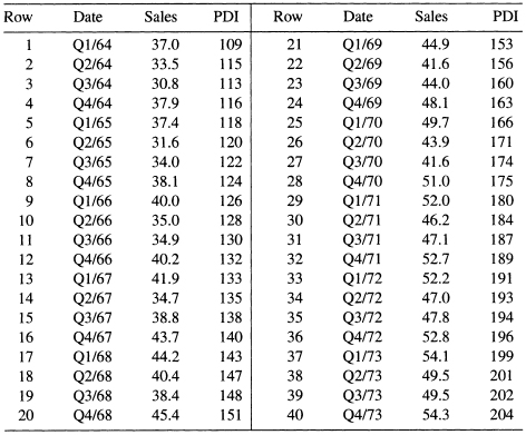
The data set we use as an example here, referred to as the Ski Sales data, is shown in Table 5.11 and can be obtained from the book's Web Site. The data consist of two variables: the sales, S, in millions for a firm that manufactures skis and related equipment for the years 1964–1973, and personal disposable income, PDI.⁵ Each of these variables is measured quarterly. We use these data in Chapter 8 to illustrate the problem of correlated errors. The model is an equation that relates S to PDI,

where S_t, is sales in millions in the tth period and PDI_t is the corresponding personal disposable income. Our approach here is to assume the existence of a seasonal effect on sales that is determined on a quarterly basis. To measure this effect we may define indicator variables to characterize the seasonality. Since we have four quarters, we define three indicator variables, Z₁, Z₂, and Z₃, where

The analysis and interpretation of this data set are left to the reader. The authors have analyzed these data and found that there are actually only two seasons. (See the discussion of these sales data in Chapter 8 for an analysis using only one indicator variable, two seasons.) See Kmenta (1986) for further discussion on using indicator variables for analyzing seasonality.

5.7 STABILITY OF REGRESSION PARAMETERS OVER TIME

Indicator variables may also be used to analyze the stability of regression coefficients over time or to test for structural change. We consider an extension of the system of regressions problem when data are available on a cross-section of observations and over time. Our objective is to analyze the constancy of the relationships over time. The methods described here are suitable for intertemporal and interspatial comparisons. To outline the method we use the Education Expenditure data shown in Tables 5.12–5.14. The measured variables for the 50 states are:

Y	Per capita expenditure on public education
X1	Per capita personal income
X2	Number of residents per thousand under 18 years of age
X3	Number of people per thousand residing in urban areas

The variable Region is a categorical variable representing geographical regions (1 = Northeast, 2 = North Central, 3 = South, 4 = West). This data set is used in Chapter 7 to demonstrate methods of dealing with heteroscedasticity in multiple regression and to analyze the effects of regional characteristics on the regression relationships. Here we focus on the stability of the expenditure relationship with respect to time.

Table 5.11 Disposable Income and Ski Sales for Years 1964–1973

Data have been developed on the four variables described above for each state in 1960, 1970, and 1975. Assuming that the relationship can be identically specified in each of the three years,⁶ the analysis of stability can be carried out by evaluating the variation in the estimated regression coefficients over time. Working with the pooled data set of 150 observations (50 states each in 3 years) we define two indicator variables, T₁ and T₂, where

Using Y to represent per capita expenditure on schools, the model takes the form

From the definitions of T₁ and T₂, the above model is equivalent to

As noted earlier, this method of analysis necessarily implies that the variability about the regression function is assumed to be equal for all three years. One formal hypothesis of interest is

which implies that the regression system has remained unchanged throughout the period of investigation (1960–1975).

The data for this example, which we refer to as the Education Expenditures data, appear in Tables 5.12, 5.13, and 5.14 and can be obtained from the book's Web Site. The reader is invited to perform the analysis described above as an exercise.

EXERCISES

5.1 Using the model defined in (5.6):

(a) Check to see if the usual least squares assumptions hold.

(b) Test H₀ : γ = 0 using the F-test.

(c) Test H₀ : γ = 0 using the t-test.

(d) Verify the equivalence of the two tests above.

5.2 Using the model defined in (5.8):

(a) Check to see if the usual least squares assumptions hold.

(b) Test H₀ : δ = 0 using the F-test.

(c) Test H₀ : δ = 0 using the t-test,

(d) Verify the equivalence of the two tests above.

5.3 Perform a thorough analysis of the Ski Sales data in Table 5.11 using the ideas presented in Section 5.6.

5.4 Perform a thorough analysis of the Education Expenditures data in Tables 5.12, 5.13, and 5.14 using the ideas presented in Section 5.7.

Table 5.12 Education Expenditures Data (1960)

Table 5.13 Education Expenditures Data (1970)

Table 5.14 Education Expenditures Data (1975)

Table 5.15 Corn Yields by Fertilizer Group

5.5 Three types of fertilizer are to be tested to see which one yields more com crop. Forty similar plots of land were available for testing purposes. The 40 plots are divided at random into four groups, ten plots in each group. Fertilizer 1 was applied to each of the ten corn plots in Group 1. Similarly, Fertilizers 2 and 3 were applied to the plots in Groups 2 and 3, respectively. The com plants in Group 4 were not given any fertilizer; it will serve as the control group. Table 5.15 gives the corn yield y_ij for each of the forty plots.

(a) Create three indicator variables F₁, F₂, F₃, one for each of the three fertilizer groups.

(b) Fit the model y_ij = μ₀ + μ₁F_i1 + μ₂F_i2 + μ₃F_i3 + ε_ij.

(c) Test the hypothesis that, on the average, none of the three types of fertilizer has an effect on com crops. Specify the hypothesis to be tested, the test used, and your conclusions at the 5% significance level.

(d) Test the hypothesis that, on the average, the three types of fertilizer have equal effects on corn crop but different from that of the control group. Specify the hypothesis to be tested, the test used, and your conclusions at the 5% significance level.

(e) Which of the three fertilizers has the greatest effects on corn yield?

5.6 In a statistics course personal information was collected on all the students for class analysis. Data on age (in years), height (in inches), and weight (in pounds) of the students are given in Table 5.16 and can be obtained from the book's Web Site. The sex of each student is also noted and coded as 1 for women and 0 for men. We want to study the relationship between the height and weight of students. Weight is taken as the response variable, and the height as the predictor variable.

(a) Do you agree or do you think the roles of the variables should be reversed?

(b) Is a single equation adequate to describe the relationship between height and weight for the two groups of students? Examine the standardized residual plot from the model fitted to the pooled data, distinguishing between the male and female students.

Table 5.16 Class Data on Age (in Years), Height (in Inches), Weight (in Pounds), and Sex (1 = Female, 0 =Male)

(c) Find the best model that describes the relationship between the weight and the height of students. Use interaction variables and the methodology described in this chapter.

(d) Do you think we should include age as a variable to predict weight? Give an intuitive justification for your answer.

5.7 Presidential Election Data (1916–1996): The data in Table 5.17 were kindly provided by Professor Ray Fair of Yale University, who has found that the proportion of votes obtained by a presidential candidate in a United States presidential election can be predicted accurately by three macroeconomic variables, incumbency, and a variable which indicates whether the election was held during or just after a war. The variables considered are given in Table 5.18. All growth rates are annual rates in percentage points. Consider fitting the initial model

Table 5.17 Presidential Election Data (1916–1996)

to the data.

(a) Do we need to keep the variable I in the above model?

(b) Do we need to keep the interaction variable (G · I) in the above model?

(c) Examine different models to produce the model or models that might be expected to perform best in predicting future presidential elections. Include interaction terms if needed.

Table 5.18 Variables for the Presidential Election Data (1916–1996) in Table 5.17