
Chapter 3. Drawing in Space: Geometric Primitives and Buffers
WHAT YOU’LL LEARN IN THIS CHAPTER:

If you’ve ever had a chemistry class (and probably even if you haven’t), you know that all matter consists of atoms and that all atoms consist of only three things: protons, neutrons, and electrons. All the materials and substances you have ever come into contact with—from the petals of a rose to the sand on the beach—are just different arrangements of these three fundamental building blocks. Although this explanation is a little oversimplified for almost anyone beyond the third or fourth grade, it demonstrates a powerful principle: With just a few simple building blocks, you can create highly complex and beautiful structures.
The connection is fairly obvious. Objects and scenes that you create with OpenGL also consist of smaller, simpler shapes, arranged and combined in various and unique ways. This chapter explores these building blocks of 3D objects, called primitives. All primitives in OpenGL are one-, two-, or three-dimensional objects, ranging from single points to lines and complex polygons. In this chapter, you learn everything you need to know to draw objects in three dimensions from these simpler shapes.
Drawing Points in 3D
When you first learned to draw any kind of graphics on any computer system, you probably started with pixels. A pixel is the smallest element on your computer monitor, and on color systems that pixel can be any one of many available colors. This is computer graphics at its simplest: Draw a point somewhere on the screen, and make it a specific color. Then build on this simple concept, using your favorite computer language to produce lines, polygons, circles, and other shapes and graphics. Perhaps even a GUI...
With OpenGL, however, drawing on the computer screen is fundamentally different. You’re not concerned with physical screen coordinates and pixels, but rather positional coordinates in your viewing volume. You let OpenGL worry about how to get your points, lines, and everything else projected from your established 3D space to the 2D image made by your computer screen.
This chapter and the next cover the most fundamental concepts of OpenGL or any 3D graphics toolkit. In the upcoming chapter, we provide substantial detail about how this transformation from 3D space to the 2D landscape of your computer monitor takes place, as well as how to transform (rotate, translate, and scale) your objects. For now, we take this capability for granted to focus on plotting and drawing in a 3D coordinate system. This approach might seem backward, but if you first know how to draw something and then worry about all the ways to manipulate your drawings, the material in Chapter 4, “Geometric Transformations: The Pipeline,” is more interesting and easier to learn. When you have a solid understanding of graphics primitives and coordinate transformations, you will be able to quickly master any 3D graphics language or API.
Setting Up a 3D Canvas
Figure 3.1 shows a simple viewing volume that we use for the examples in this chapter. The area enclosed by this volume is a Cartesian coordinate space that ranges from –100 to +100 on all three axes—x, y, and z. (For a review of Cartesian coordinates, see Chapter 1, “Introduction to 3D Graphics and OpenGL.”) Think of this viewing volume as your three-dimensional canvas on which you draw with OpenGL commands and functions.
Figure 3.1. A Cartesian viewing volume measuring 100×100×100.

We established this volume with a call to glOrtho, much as we did for others in the preceding chapter. Listing 3.1 shows the code for the ChangeSize function that is called when the window is sized (including when it is first created). This code looks a little different from that in the preceding chapter, and you’ll notice some unfamiliar functions (glMatrixMode, glLoadIdentity). We’ll spend more time on these functions in Chapter 4, exploring their operation in more detail.
Listing 3.1. Code to Establish the Viewing Volume in Figure 3.1

A 3D Point: The Vertex
To specify a drawing point in this 3D “palette,” we use the OpenGL function glVertex—without a doubt one of the most used functions in all the OpenGL API. This is the “lowest common denominator” of all the OpenGL primitives: a single point in space. The glVertex function can take from one (a pointer) to four parameters of any numerical type, from bytes to doubles, subject to the naming conventions discussed in Chapter 2, “Using OpenGL.”
The following single line of code specifies a point in our coordinate system located 50 units along the x-axis, 50 units along the y-axis, and 0 units along the z-axis:
glVertex3f(50.0f, 50.0f, 0.0f);
Figure 3.2 illustrates this point. Here, we chose to represent the coordinates as floating-point values, as we do for the remainder of the book. Also, the form of glVertex that we use takes three arguments for the x, y, and z coordinate values, respectively.
Figure 3.2. The point (50,50,0) as specified by glVertex3f(50.0f, 50.0f, 0.0f).

Two other forms of glVertex take two and four arguments, respectively. We can represent the same point in Figure 3.2 with this code:
glVertex2f(50.0f, 50.0f);
This form of glVertex takes only two arguments, specifying the x and y values, and assumes the z coordinate to be 0.0 always.
The form of glVertex taking four arguments, glVertex4, uses a fourth coordinate value, w (set to 1.0 by default when not specified) for scaling purposes. You will learn more about this coordinate in Chapter 4 when we spend more time exploring coordinate transformations.
Draw Something!
Now, we have a way of specifying a point in space to OpenGL. What can we make of it, and how do we tell OpenGL what to do with it? Is this vertex a point that should just be plotted? Is it the endpoint of a line or the corner of a cube? The geometric definition of a vertex is not just a point in space, but rather the point at which an intersection of two lines or curves occurs. This is the essence of primitives.
A primitive is simply the interpretation of a set or list of vertices into some shape drawn on the screen. There are 10 primitives in OpenGL, from a simple point drawn in space to a closed polygon of any number of sides. One way to draw primitives is to use the glBegin command to tell OpenGL to begin interpreting a list of vertices as a particular primitive. You then end the list of vertices for that primitive with the glEnd command. Kind of intuitive, don’t you think?
Drawing Points
Let’s begin with the first and simplest of primitives: points. Look at the following code:
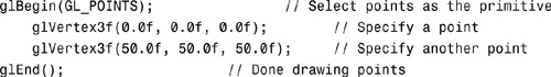
The argument to glBegin, GL_POINTS tells OpenGL that the following vertices are to be interpreted and drawn as points. Two vertices are listed here, which translates to two specific points, both of which would be drawn.
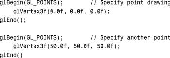
This example brings up an important point about glBegin and glEnd: You can list multiple primitives between calls as long as they are for the same primitive type. In this way, with a single glBegin/glEnd sequence, you can include as many primitives as you like. This next code segment is wasteful and will execute more slowly than the preceding code:
Our First Example
The code in Listing 3.2 draws some points in our 3D environment. It uses some simple trigonometry to draw a series of points that form a corkscrew path up the z-axis. This code is from the POINTS program, which is in the source distribution for this chapter. All the sample programs use the framework we established in Chapter 2. Notice that in the SetupRC function, we are setting the current drawing color to green.
Listing 3.2. Rendering Code to Produce a Spring-Shaped Path of Points


Only the code between calls to glBegin and glEnd is important for our purpose in this and the other examples for this chapter. This code calculates the x and y coordinates for an angle that spins between 0° and 360° three times. We express this programmatically in radians rather than degrees; if you don’t know trigonometry, you can take our word for it. If you’re interested, see the box “The Trigonometry of Radians/Degrees.” Each time a point is drawn, the z value is increased slightly. When this program is run, all you see is a circle of points because you are initially looking directly down the z-axis. To see the effect, use the arrow keys to spin the drawing around the x- and y-axes. The effect is illustrated in Figure 3.3.
Figure 3.3. Output from the POINTS sample program.


Setting the Point Size
When you draw a single point, the size of the point is one pixel by default. You can change this size with the function glPointSize:
void glPointSize(GLfloat size);
The glPointSize function takes a single parameter that specifies the approximate diameter in pixels of the point drawn. Not all point sizes are supported, however, and you should make sure the point size you specify is available. Use the following code to get the range of point sizes and the smallest interval between them:
GLfloat sizes[2]; // Store supported point size range
GLfloat step; // Store supported point size increments
// Get supported point size range and step size
glGetFloatv(GL_POINT_SIZE_RANGE,sizes);
glGetFloatv(GL_POINT_SIZE_GRANULARITY,&step);
Here, the sizes array will contain two elements that contain the smallest and largest valid value for glPointsize. In addition, the variable step will hold the smallest step size allowable between the point sizes. The OpenGL specification requires only that one point size, 1.0, be supported. The Microsoft software implementation of OpenGL, for example, allows for point sizes from 0.5 to 10.0, with 0.125 the smallest step size. Specifying a size out of range is not interpreted as an error. Instead, the largest or smallest supported size is used, whichever is closest to the value specified.
By default, points, unlike other geometry, are not affected by the perspective division. That is, they do not become smaller when they are further from the viewpoint, and they do not become larger as they move closer. Points are also always square pixels, even if you use glPointSize to increase the size of the points. You just get bigger squares! To get round points, you must draw them antialiased (coming up in Chapter 6, “More on Colors and Materials”).
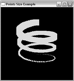
Let’s look at a sample that uses these new functions. The code in Listing 3.3 produces the same spiral shape as our first example, but this time, the point sizes are gradually increased from the smallest valid size to the largest valid size. This example is from the program POINTSZ in source distribution for this chapter. The output from POINTSZ shown in Figure 3.4 was run on Microsoft’s software implementation of OpenGL. Figure 3.5 shows the same program run on a hardware accelerator that supports much larger point sizes.
Figure 3.4. Output from the POINTSZ program.

Figure 3.5. Output from POINTSZ on hardware supporting much larger point sizes.
Listing 3.3. Code from POINTSZ That Produces a Spiral with Gradually Increasing Point Sizes


This example demonstrates a couple of important things. For starters, notice that glPointSize must be called outside the glBegin/glEnd statements. Not all OpenGL functions are valid between these function calls. Although glPointSize affects all points drawn after it, you don’t begin drawing points until you call glBegin(GL_POINTS). For a complete list of valid functions that you can call within a glBegin/glEnd sequence, see the reference section in Appendix C.
If you specify a point size larger than what is returned in the size variable, you also may notice (depending on your hardware) that OpenGL uses the largest available point size but does not keep growing. This is a general observation about OpenGL function parameters that have a valid range. Values outside the range are clamped to the range. Values too low are made the lowest valid value, and values too high are made the highest valid value.
The most obvious thing you probably noticed about the POINTSZ excerpt is that the larger point sizes are represented simply by larger cubes. This is the default behavior, but it typically is undesirable for many applications. Also, you might wonder why you can increase the point size by a value less than one. If a value of 1.0 represents one pixel, how do you draw less than a pixel, or, say, 2.5 pixels?
The answer is that the point size specified in glPointSize isn’t the exact point size in pixels, but the approximate diameter of a circle containing all the pixels that are used to draw the point. You can get OpenGL to draw the points as better points (that is, small filled circles) by enabling point smoothing. Together with line smoothing, point smoothing falls under the topic of antialiasing. Antialiasing is a technique used to smooth out jagged edges and round out corners; it is covered in more detail in Chapter 6.
Points can also be made to grow and shrink with the perspective projection, but this is not the default behavior. A feature called point parameters makes this possible, and is a bit deep for this early in the book. We will discuss point parameters along with another interesting point texturing feature called point sprites in Chapter 9, “Texture Mapping: Beyond the Basics.”
Drawing Lines in 3D
The GL_POINTS primitive we have been using thus far is reasonably straightforward; for each vertex specified, it draws a point. The next logical step is to specify two vertices and draw a line between them. This is exactly what the next primitive, GL_LINES, does. The following short section of code draws a single line between two points (0,0,0) and (50,50,50):
glBegin(GL_LINES);
glVertex3f(0.0f, 0.0f, 0.0f);
glVertex3f(50.0f, 50.0f, 50.0f);
glEnd();
Note here that two vertices specify a single primitive. For every two vertices specified, a single line is drawn. If you specify an odd number of vertices for GL_LINES, the last vertex is just ignored. Listing 3.4, from the LINES sample program, shows a more complex sample that draws a series of lines fanned around in a circle. Each point specified in this sample is paired with a point on the opposite side of a circle. The output from this program is shown in Figure 3.6.
Figure 3.6. Output from the LINES sample program.

Listing 3.4. Code from the Sample Program LINES That Displays a Series of Lines Fanned in a Circle

Line Strips and Loops
The next two OpenGL primitives build on GL_LINES by allowing you to specify a list of vertices through which a line is drawn. When you specify GL_LINE_STRIP, a line is drawn from one vertex to the next in a continuous segment. The following code draws two lines in the xy plane that are specified by three vertices. Figure 3.7 shows an example.
glBegin(GL_LINE_STRIP);
glVertex3f(0.0f, 0.0f, 0.0f); // V0
glVertex3f(50.0f, 50.0f, 0.0f); // V1
glVertex3f(50.0f, 100.0f, 0.0f); // V2
glEnd();
Figure 3.7. An example of a GL_LINE_STRIP specified by three vertices.

The last line-based primitive is GL_LINE_LOOP. This primitive behaves just like GL_LINE_STRIP, but one final line is drawn between the last vertex specified and the first one specified. This is an easy way to draw a closed-line figure. Figure 3.8 shows a GL_LINE_LOOP drawn using the same vertices as for the GL_LINE_STRIP in Figure 3.7.
Figure 3.8. The same vertices from Figure 3.7 used by a GL_LINE_LOOP primitive.

Approximating Curves with Straight Lines
The POINTS sample program, shown earlier in Figure 3.3, showed you how to plot points along a spring-shaped path. You might have been tempted to push the points closer and closer together (by setting smaller values for the angle increment) to create a smooth spring-shaped curve instead of the broken points that only approximated the shape. This perfectly valid operation can move quite slowly for larger and more complex curves with thousands of points.
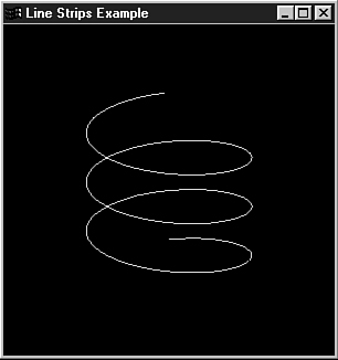
A better way of approximating a curve is to use GL_LINE_STRIP to play connect-the-dots. As the dots move closer together, a smoother curve materializes without you having to specify all those points. Listing 3.5 shows the code from Listing 3.2, with GL_POINTS replaced by GL_LINE_STRIP. The output from this new program, LSTRIPS, is shown in Figure 3.9. As you can see, the approximation of the curve is quite good. You will find this handy technique almost ubiquitous among OpenGL programs.
Figure 3.9. Output from the LSTRIPS program approximating a smooth curve.
Listing 3.5. Code from the Sample Program LSTRIPS, Demonstrating Line Strips

Setting the Line Width
Just as you can set different point sizes, you can also specify various line widths when drawing lines by using the glLineWidth function:
void glLineWidth(GLfloat width);
The glLineWidth function takes a single parameter that specifies the approximate width, in pixels, of the line drawn. Just as with point sizes, not all line widths are supported, and you should make sure that the line width you want to specify is available. Use the following code to get the range of line widths and the smallest interval between them:
GLfloat sizes[2]; // Store supported line width range
GLfloat step; // Store supported line width increments
// Get supported line width range and step size
glGetFloatv(GL_LINE_WIDTH_RANGE,sizes);
glGetFloatv(GL_LINE_WIDTH_GRANULARITY,&step);
Here, the sizes array will contain two elements that contain the smallest and largest valid value for glLineWidth. In addition, the variable step will hold the smallest step size allowable between the line widths. The OpenGL specification requires only that one line width, 1.0, be supported. The Microsoft implementation of OpenGL allows for line widths from 0.5 to 10.0, with 0.125 the smallest step size.
Listing 3.6 shows code for a more substantial example of glLineWidth. It’s from the program LINESW and draws 10 lines of varying widths. It starts at the bottom of the window at –90 on the y-axis and climbs the y-axis 20 units for each new line. Every time it draws a new line, it increases the line width by 1. Figure 3.10 shows the output for this program.
Figure 3.10. A demonstration of glLineWidth from the LINESW program.

Listing 3.6. Drawing Lines of Various Widths

Notice that we used glVertex2f this time instead of glVertex3f to specify the coordinates for the lines. As mentioned, using this technique is only a convenience because we are drawing in the xy plane, with a z value of 0. To see that you are still drawing lines in three dimensions, simply use the arrow keys to spin your lines around. You easily see that all the lines lie on a single plane.
Line Stippling
In addition to changing line widths, you can create lines with a dotted or dashed pattern, called stippling. To use line stippling, you must first enable stippling with a call to
glEnable(GL_LINE_STIPPLE);
Then the function glLineStipple establishes the pattern that the lines use for drawing:
void glLineStipple(GLint factor, GLushort pattern);
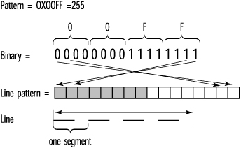
The pattern parameter is a 16-bit value that specifies a pattern to use when drawing the lines. Each bit represents a section of the line segment that is either on or off. By default, each bit corresponds to a single pixel, but the factor parameter serves as a multiplier to increase the width of the pattern. For example, setting factor to 5 causes each bit in the pattern to represent five pixels in a row that are either on or off. Furthermore, bit 0 (the least significant bit) of the pattern is used first to specify the line. Figure 3.11 illustrates a sample bit pattern applied to a line segment.
Figure 3.11. A stipple pattern is used to construct a line segment.
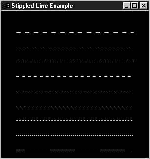
Listing 3.7 shows a sample of using a stippling pattern that is just a series of alternating on and off bits (0101010101010101). This code is taken from the LSTIPPLE program, which draws 10 lines from the bottom of the window up the y-axis to the top. Each line is stippled with the pattern 0x5555, but for each new line, the pattern multiplier is increased by 1. You can clearly see the effects of the widened stipple pattern in Figure 3.12.
Figure 3.12. Output from the LSTIPPLE program.
Listing 3.7. Code from LSTIPPLE That Demonstrates the Effect of factor on the Bit Pattern

Just the ability to draw points and lines in 3D gives you a significant set of tools for creating your own 3D masterpiece. Figure 3.13 shows a 3D weather mapping program with an OpenGL-rendered map that is rendered entirely of solid and stippled line strips.
Figure 3.13. A 3D map rendered with solid and stippled lines.

Drawing Triangles in 3D
You’ve seen how to draw points and lines and even how to draw some enclosed polygons with GL_LINE_LOOP. With just these primitives, you could easily draw any shape possible in three dimensions. You could, for example, draw six squares and arrange them so they form the sides of a cube.
You might have noticed, however, that any shapes you create with these primitives are not filled with any color; after all, you are drawing only lines. In fact, arranging six squares produces just a wireframe cube, not a solid cube. To draw a solid surface, you need more than just points and lines; you need polygons. A polygon is a closed shape that may or may not be filled with the currently selected color, and it is the basis of all solid-object composition in OpenGL.
Triangles: Your First Polygon
The simplest polygon possible is the triangle, with only three sides. The GL_TRIANGLES primitive draws triangles by connecting three vertices together. The following code draws two triangles using three vertices each, as shown in Figure 3.14:
glBegin(GL_TRIANGLES);
glVertex2f(0.0f, 0.0f); // V0
glVertex2f(25.0f, 25.0f); // V1
glVertex2f(50.0f, 0.0f); // V2
glVertex2f(-50.0f, 0.0f); // V3
glVertex2f(-75.0f, 50.0f); // V4
glVertex2f(-25.0f, 0.0f); // V5
glEnd();
Figure 3.14. Two triangles drawn using GL_TRIANGLES.
Winding
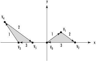
An important characteristic of any polygonal primitive is illustrated in Figure 3.14. Notice the arrows on the lines that connect the vertices. When the first triangle is drawn, the lines are drawn from V0 to V1, then to V2, and finally back to V0 to close the triangle. This path is in the order in which the vertices are specified, and for this example, that order is clockwise from your point of view. The same directional characteristic is present for the second triangle as well.
The combination of order and direction in which the vertices are specified is called winding. The triangles in Figure 3.14 are said to have clockwise winding because they are literally wound in the clockwise direction. If we reverse the positions of V4 and V5 on the triangle on the left, we get counterclockwise winding. Figure 3.15 shows two triangles, each with opposite windings.
Figure 3.15. Two triangles with different windings.

OpenGL, by default, considers polygons that have counterclockwise winding to be front facing. This means that the triangle on the left in Figure 3.15 shows the front of the triangle, and the one on the right shows the back of the triangle.
Why is this issue important? As you will soon see, you will often want to give the front and back of a polygon different physical characteristics. You can hide the back of a polygon altogether or give it a different color and reflective property (see Chapter 5, “Color, Materials, and Lighting: The Basics”). It’s important to keep the winding of all polygons in a scene consistent, using front-facing polygons to draw the outside surface of any solid objects. In the upcoming section on solid objects, we demonstrate this principle using some models that are more complex.
If you need to reverse the default behavior of OpenGL, you can do so by calling the following function:
glFrontFace(GL_CW);
The GL_CW parameter tells OpenGL that clockwise-wound polygons are to be considered front facing. To change back to counterclockwise winding for the front face, use GL_CCW.
Triangle Strips
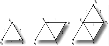
For many surfaces and shapes, you need to draw several connected triangles. You can save a lot of time by drawing a strip of connected triangles with the GL_TRIANGLE_STRIP primitive. Figure 3.16 shows the progression of a strip of three triangles specified by a set of five vertices numbered V0 through V4. Here, you see that the vertices are not necessarily traversed in the same order in which they were specified. The reason for this is to preserve the winding (counterclockwise) of each triangle. The pattern is V0, V1, V2; then V2, V1, V3; then V2, V3, V4; and so on.
Figure 3.16. The progression of a GL_TRIANGLE_STRIP.
For the rest of the discussion of polygonal primitives, we don’t show any more code fragments to demonstrate the vertices and the glBegin statements. You should have the swing of things by now. Later, when we have a real sample program to work with, we’ll resume the examples.
There are two advantages to using a strip of triangles instead of specifying each triangle separately. First, after specifying the first three vertices for the initial triangle, you need to specify only a single point for each additional triangle. This saves a lot of program or data storage space when you have many triangles to draw. The second advantage is mathematical performance and bandwidth savings. Fewer vertices means a faster transfer from your computer’s memory to your graphics card and fewer vertex transformations (see Chapter 4).
Triangle Fans
In addition to triangle strips, you can use GL_TRIANGLE_FAN to produce a group of connected triangles that fan around a central point. Figure 3.17 shows a fan of three triangles produced by specifying four vertices. The first vertex, V0, forms the origin of the fan. After the first three vertices are used to draw the initial triangle, all subsequent vertices are used with the origin (V0) and the vertex immediately preceding it (Vn–1) to form the next triangle.
Figure 3.17. The progression of GL_TRIANGLE_FAN.

Building Solid Objects
Composing a solid object out of triangles (or any other polygon) involves more than assembling a series of vertices in a 3D coordinate space. Let’s examine the sample program TRIANGLE, which uses two triangle fans to create a cone in our viewing volume. The first fan produces the cone shape, using the first vertex as the point of the cone and the remaining vertices as points along a circle farther down the z-axis. The second fan forms a circle and lies entirely in the xy plane, making up the bottom surface of the cone.
The output from TRIANGLE is shown in Figure 3.18. Here, you are looking directly down the z-axis and can see only a circle composed of a fan of triangles. The individual triangles are emphasized by coloring them alternately green and red.
Figure 3.18. Initial output from the TRIANGLE sample program.

The code for the SetupRC and RenderScene functions is shown in Listing 3.8. (This listing contains some unfamiliar variables and specifiers that are explained shortly.) This program demonstrates several aspects of composing 3D objects. Right-click in the window, and you will notice an Effects menu; it will be used to enable and disable some 3D drawing features so that we can explore some of the characteristics of 3D object creation. We’ll describe these features as we progress.
Listing 3.8. SetupRC and RenderScene Code for the TRIANGLE Sample Program


Setting Polygon Colors
Until now, we have set the current color only once and drawn only a single shape. Now, with multiple polygons, things get slightly more interesting. We want to use different colors so we can see our work more easily. Colors are actually specified per vertex, not per polygon. The shading model affects whether the polygon is solidly colored (using the current color selected when the last vertex was specified) or smoothly shaded between the colors specified for each vertex.
The line
glShadeModel(GL_FLAT);
tells OpenGL to fill the polygons with the solid color that was current when the polygon’s last vertex was specified. This is why we can simply change the current color to red or green before specifying the next vertex in our triangle fan. On the other hand, the line
glShadeModel(GL_SMOOTH);
would tell OpenGL to shade the triangles smoothly from each vertex, attempting to interpolate the colors between those specified for each vertex. You’ll learn much more about color and shading in Chapter 5.
Hidden Surface Removal
Hold down one of the arrow keys to spin the cone around, and don’t select anything from the Effects menu yet. You’ll notice something unsettling: The cone appears to be swinging back and forth plus and minus 180°, with the bottom of the cone always facing you, but not rotating a full 360°. Figure 3.19 shows this effect more clearly.
Figure 3.19. The rotating cone appears to be wobbling back and forth.

This wobbling happens because the bottom of the cone is drawn after the sides of the cone are drawn. No matter how the cone is oriented, the bottom is drawn on top of it, producing the “wobbling” illusion. This effect is not limited to the various sides and parts of an object. If more than one object is drawn and one is in front of the other (from the viewer’s perspective), the last object drawn still appears over the previously drawn object.
You can correct this peculiarity with a simple feature called depth testing. Depth testing is an effective technique for hidden surface removal, and OpenGL has functions that do this for you behind the scenes. The concept is simple: When a pixel is drawn, it is assigned a value (called the z value) that denotes its distance from the viewer’s perspective. Later, when another pixel needs to be drawn to that screen location, the new pixel’s z value is compared to that of the pixel that is already stored there. If the new pixel’s z value is higher, it is closer to the viewer and thus in front of the previous pixel, so the previous pixel is obscured by the new pixel. If the new pixel’s z value is lower, it must be behind the existing pixel and thus is not obscured. This maneuver is accomplished internally by a depth buffer with storage for a depth value for every pixel on the screen. Almost all the samples in this book use depth testing.
You should request a depth buffer when you set up your OpenGL window with GLUT. For example, you can request a color and a depth buffer like this:
glutInitDisplayMode(GLUT_DOUBLE | GLUT_RGBA | GLUT_DEPTH);
To enable depth testing, simply call
glEnable(GL_DEPTH_TEST);
If you do not have a depth buffer, then enabling depth testing will just be ignored. Depth testing is enabled in Listing 3.8 when the bDepth variable is set to True, and it is disabled if bDepth is False:
// Enable depth testing if flag is set
if(bDepth)
glEnable(GL_DEPTH_TEST);
else
glDisable(GL_DEPTH_TEST);
The bDepth variable is set when you select Depth Test from the Effects menu. In addition, the depth buffer must be cleared each time the scene is rendered. The depth buffer is analogous to the color buffer in that it contains information about the distance of the pixels from the observer. This information is used to determine whether any pixels are hidden by pixels closer to the observer:
// Clear the window and the depth buffer
glClear(GL_COLOR_BUFFER_BIT | GL_DEPTH_BUFFER_BIT);
A right-click with the mouse opens a pop-up menu that allows you to toggle depth testing on and off. Figure 3.20 shows the TRIANGLE program with depth testing enabled. It also shows the cone with the bottom correctly hidden behind the sides. You can see that depth testing is practically a prerequisite for creating 3D objects out of solid polygons.
Figure 3.20. The bottom of the cone is now correctly placed behind the sides for this orientation.

Culling: Hiding Surfaces for Performance
You can see that there are obvious visual advantages to not drawing a surface that is obstructed by another. Even so, you pay some performance overhead because every pixel drawn must be compared with the previous pixel’s z value. Sometimes, however, you know that a surface will never be drawn anyway, so why specify it? Culling is the term used to describe the technique of eliminating geometry that we know will never be seen. By not sending this geometry to your OpenGL driver and hardware, you can make significant performance improvements. One culling technique is backface culling, which eliminates the backsides of a surface.
In our working example, the cone is a closed surface, and we never see the inside. OpenGL is actually (internally) drawing the back sides of the far side of the cone and then the front sides of the polygons facing us. Then, by a comparison of z buffer values, the far side of the cone is either overwritten or ignored. Figures 3.21a and 3.21b show our cone at a particular orientation with depth testing turned on (a) and off (b). Notice that the green and red triangles that make up the cone sides change when depth testing is enabled. Without depth testing, the sides of the triangles at the far side of the cone show through.
Figure 3.21A. With depth testing.

Figure 3.21B. Without depth testing.

Earlier in the chapter, we explained how OpenGL uses winding to determine the front and back sides of polygons and that it is important to keep the polygons that define the outside of our objects wound in a consistent direction. This consistency is what allows us to tell OpenGL to render only the front, only the back, or both sides of polygons. By eliminating the back sides of the polygons, we can drastically reduce the amount of processing necessary to render the image. Even though depth testing will eliminate the appearance of the inside of objects, internally OpenGL must take them into account unless we explicitly tell it not to.
Backface culling is enabled or disabled for our program via the following code from Listing 3.8:
// Clockwise-wound polygons are front facing; this is reversed
// because we are using triangle fans
glFrontFace(GL_CW);
...
...
// Turn culling on if flag is set
if(bCull)
glEnable(GL_CULL_FACE);
else
glDisable(GL_CULL_FACE);
Note that we first changed the definition of front-facing polygons to assume clockwise winding (because our triangle fans are all wound clockwise).
Figure 3.22 demonstrates that the bottom of the cone is gone when culling is enabled. The reason is that we didn’t follow our own rule about all the surface polygons having the same winding. The triangle fan that makes up the bottom of the cone is wound clockwise, like the fan that makes up the sides of the cone, but the front side of the cone’s bottom section is then facing the inside (see Figure 3.23).
Figure 3.22. The bottom of the cone is culled because the front-facing triangles are inside.

Figure 3.23. How the cone was assembled from two triangle fans.

We could have corrected this problem by changing the winding rule, by calling
glFrontFace(GL_CCW);
just before we drew the second triangle fan. But in this example, we wanted to make it easy for you to see culling in action, as well as set up for our next demonstration of polygon tweaking.
Polygon Modes
Polygons don’t have to be filled with the current color. By default, polygons are drawn solid, but you can change this behavior by specifying that polygons are to be drawn as outlines or just points (only the vertices are plotted). The function glPolygonMode allows polygons to be rendered as filled solids, as outlines, or as points only. In addition, you can apply this rendering mode to both sides of the polygons or only to the front or back. The following code from Listing 3.8 shows the polygon mode being set to outlines or solid, depending on the state of the Boolean variable bOutline:
// Draw back side as a polygon only, if flag is set
if(bOutline)
glPolygonMode(GL_BACK,GL_LINE);
else
glPolygonMode(GL_BACK,GL_FILL);
Figure 3.24 shows the back sides of all polygons rendered as outlines. (We had to disable culling to produce this image; otherwise, the inside would be eliminated and you would get no outlines.) Notice that the bottom of the cone is now wireframe instead of solid, and you can see up inside the cone where the inside walls are also drawn as wireframe triangles.
Figure 3.24. Using glPolygonMode to render one side of the triangles as outlines.

Other Primitives
Triangles are the preferred primitive for object composition because most OpenGL hardware specifically accelerates triangles, but they are not the only primitives available. Some hardware provides for acceleration of other shapes as well, and programmatically, using a general-purpose graphics primitive might be simpler. The remaining OpenGL primitives provide for rapid specification of a quadrilateral or quadrilateral strip, as well as a general-purpose polygon.
Four-Sided Polygons: Quads
If you add one more side to a triangle, you get a quadrilateral, or a four-sided figure. OpenGL’s GL_QUADS primitive draws a four-sided polygon. In Figure 3.25, a quad is drawn from four vertices. Note also that these quads have clockwise winding. One important rule to bear in mind when you use quads is that all four corners of the quadrilateral must lie in a plane (no bent quads!).
Figure 3.25. An example of GL_QUADS.

Quad Strips
As you can for triangle strips, you can specify a strip of connected quadrilaterals with the GL_QUAD_STRIP primitive. Figure 3.26 shows the progression of a quad strip specified by six vertices. Note that these quad strips maintain a clockwise winding.
Figure 3.26. The progression of GL_QUAD_STRIP.

General Polygons
The final OpenGL primitive is the GL_POLYGON, which you can use to draw a polygon having any number of sides. Figure 3.27 shows a polygon consisting of five vertices. Polygons, like quads, must have all vertices on the same plane. An easy way around this rule is to substitute GL_TRIANGLE_FAN for GL_POLYGON!
Figure 3.27. The progression of GL_POLYGON.

Filling Polygons, or Stippling Revisited
There are two methods for applying a pattern to solid polygons. The customary method is texture mapping, in which an image is mapped to the surface of a polygon, and this is covered in Chapter 8, “Texture Mapping: The Basics.” Another way is to specify a stippling pattern, as we did for lines. A polygon stipple pattern is nothing more than a 32×32 monochrome bitmap that is used for the fill pattern.
To enable polygon stippling, call
glEnable(GL_POLYGON_STIPPLE);
and then call
glPolygonStipple(pBitmap);
pBitmap is a pointer to a data area containing the stipple pattern. Hereafter, all polygons are filled using the pattern specified by pBitmap (GLubyte *). This pattern is similar to that used by line stippling, except the buffer is large enough to hold a 32-by-32-bit pattern. Also, the bits are read with the most significant bit (MSB) first, which is just the opposite of line stipple patterns. Figure 3.28 shows a bit pattern for a campfire that we use for a stipple pattern.
Figure 3.28. Building a polygon stipple pattern.

To construct a mask to represent this pattern, we store one row at a time from the bottom up. Fortunately, unlike line stipple patterns, the data is, by default, interpreted just as it is stored, with the most significant bit read first. Each byte can then be read from left to right and stored in an array of GLubyte large enough to hold 32 rows of 4 bytes apiece.
Listing 3.9 shows the code used to store this pattern. Each row of the array represents a row from Figure 3.28. The first row in the array is the last row of the figure, and so on, up to the last row of the array and the first row of the figure.
Listing 3.9. Mask Definition for the Campfire in Figure 3.28

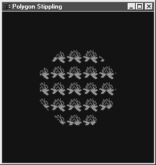
To make use of this stipple pattern, we must first enable polygon stippling and then specify this pattern as the stipple pattern. The PSTIPPLE sample program does this and then draws an octagon using the stipple pattern. Listing 3.10 shows the pertinent code, and Figure 3.29 shows the output from PSTIPPLE.
Figure 3.29. Output from the PSTIPPLE program.
Listing 3.10. Code from PSTIPPLE That Draws a Stippled Octagon

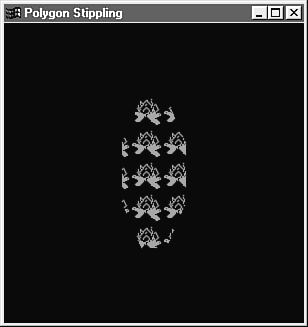
Figure 3.30 shows the octagon rotated somewhat. Notice that the stipple pattern is still used, but the pattern is not rotated with the polygon. The stipple pattern is used only for simple polygon filling onscreen. If you need to map an image to a polygon so that it mimics the polygon’s surface, you must use texture mapping (see Chapter 8).
Figure 3.30. PSTIPPLE output with the polygon rotated, showing that the stipple pattern is not rotated.
Polygon Construction Rules
When you are using many polygons to construct a complex surface, you need to remember two important rules.
The first rule is that all polygons must be planar. That is, all the vertices of the polygon must lie in a single plane, as illustrated in Figure 3.31. The polygon cannot twist or bend in space.
Figure 3.31. Planar versus nonplanar polygons.

Here is yet another good reason to use triangles. No triangle can ever be twisted so that all three points do not line up in a plane because mathematically it takes only three points to define a plane. (If you can plot an invalid triangle, aside from winding it in the wrong direction, the Nobel Prize committee might be looking for you! No cheating! Three points in a straight line do not count!)
The second rule of polygon construction is that the polygon’s edges must not intersect, and the polygon must be convex. A polygon intersects itself if any two of its lines cross. Convex means that the polygon cannot have any indentions. A more rigorous test of a convex polygon is to draw some lines through it. If any given line enters and leaves the polygon more than once, the polygon is not convex. Figure 3.32 gives examples of good and bad polygons.
Figure 3.32. Some valid and invalid primitive polygons.

Subdivision and Edges
Even though OpenGL can draw only convex polygons, there’s still a way to create a nonconvex polygon: by arranging two or more convex polygons together. For example, let’s take a four-point star, as shown in Figure 3.33. This shape is obviously not convex and thus violates OpenGL’s rules for simple polygon construction. However, the star on the right is composed of six separate triangles, which are legal polygons.
Figure 3.33. A nonconvex four-point star made up of six triangles.

When the polygons are filled, you won’t be able to see any edges and the figure will seem to be a single shape onscreen. However, if you use glPolygonMode to switch to an outline drawing, it is distracting to see all those little triangles making up some larger surface area.
OpenGL provides a special flag called an edge flag to address those distracting edges. By setting and clearing the edge flag as you specify a list of vertices, you inform OpenGL which line segments are considered border lines (lines that go around the border of your shape) and which ones are not (internal lines that shouldn’t be visible). The glEdgeFlag function takes a single parameter that sets the edge flag to True or False. When the function is set to True, any vertices that follow mark the beginning of a boundary line segment. Listing 3.11 shows an example of this from the STAR sample program.
Listing 3.11. Sample Usage of glEdgeFlag from the STAR Program

The Boolean variable bEdgeFlag is toggled on and off by a menu option to make the edges appear and disappear. If this flag is True, all edges are considered boundary edges and appear when the polygon mode is set to GL_LINES. In Figure 3.34, you can see the output from STAR, showing the wireframe star with and without edges.
Figure 3.34. The STAR program with edges enabled (left) and without edges enabled (right).

Other Buffer Tricks
You learned from Chapter 2 that OpenGL does not render (draw) these primitives directly on the screen. Instead, rendering is done in a buffer, which is later swapped to the screen. We refer to these two buffers as the front (the screen) and back color buffers. By default, OpenGL commands are rendered into the back buffer, and when you call glutSwapBuffers (or your operating system–specific buffer swap function), the front and back buffers are swapped so that you can see the rendering results. You can, however, render directly into the front buffer if you want. This capability can be useful for displaying a series of drawing commands so that you can see some object or shape actually being drawn. There are two ways to do this; both are discussed in the following section.
Using Buffer Targets
The first way to render directly into the front buffer is to just tell OpenGL that you want drawing to be done there. You do this by calling the following function:
void glDrawBuffer(Glenum mode);
Specifying GL_FRONT causes OpenGL to render to the front buffer, and GL_BACK moves rendering back to the back buffer. OpenGL implementations can support more than just a single front and back buffer for rendering, such as left and right buffers for stereo rendering, and auxiliary buffers. These other buffers are documented further in Appendix C, “API Reference.”
The second way to render to the front buffer is to simply not request double-buffered rendering when OpenGL is initialized. OpenGL is initialized differently on each OS platform, but with GLUT, we initialize our display mode for RGB color and double-buffered rendering with the following line of code:
glutInitDisplayMode(GLUT_DOUBLE | GLUT_RGB);
To get single-buffered rendering, you simply omit the bit flag GLUT_DOUBLE, as shown here:
glutInitDisplayMode(GLUT_RGB);
When you do single-buffered rendering, it is important to call either glFlush or glFinish whenever you want to see the results actually drawn to screen. A buffer swap implicitly performs a flush of the pipeline and waits for rendering to complete before the swap actually occurs. We’ll discuss the mechanics of this process in more detail in Chapter 11, “It’s All About the Pipeline: Faster Geometry Throughput.”
Listing 3.12 shows the drawing code for the sample program SINGLE. This example uses a single rendering buffer to draw a series of points spiraling out from the center of the window. The RenderScene function is called repeatedly and uses static variables to cycle through a simple animation. The output of the SINGLE sample program is shown in Figure 3.35.
Figure 3.35. Output from the single-buffered rendering example.

Listing 3.12. Drawing Code for the SINGLE Sample

Manipulating the Depth Buffer
The color buffers are not the only buffers that OpenGL renders into. In the preceding chapter, we mentioned other buffer targets, including the depth buffer. However, the depth buffer is filled with depth values instead of color values. Requesting a depth buffer with GLUT is as simple as adding the GLUT_DEPTH bit flag when initializing the display mode:
glutInitDisplayMode(GLUT_RGB | GLUT_DOUBLE | GLUT_DEPTH);
You’ve already seen that enabling the use of the depth buffer for depth testing is as easy as calling the following:
glEnable(GL_DEPTH_TEST);
Even when depth testing is not enabled, if a depth buffer is created, OpenGL will write corresponding depth values for all color fragments that go into the color buffer. Sometimes, though, you may want to temporarily turn off writing values to the depth buffer as well as depth testing. You can do this with the function glDepthMask:
void glDepthMask(GLboolean mask);
Setting the mask to GL_FALSE disables writes to the depth buffer but does not disable depth testing from being performed using any values that have already been written to the depth buffer. Calling this function with GL_TRUE re-enables writing to the depth buffer, which is the default state. Masking color writes is also possible but is a bit more involved; it’s mentioned in Chapter 6.
Cutting It Out with Scissors
One way to improve rendering performance is to update only the portion of the screen that has changed. You may also need to restrict OpenGL rendering to a smaller rectangular region inside the window. OpenGL allows you to specify a scissor rectangle within your window where rendering can take place. By default, the scissor rectangle is the size of the window, and no scissor test takes place. You turn on the scissor test with the ubiquitous glEnable function:
glEnable(GL_SCISSOR_TEST);
You can, of course, turn off the scissor test again with the corresponding glDisable function call. The rectangle within the window where rendering is performed, called the scissor box, is specified in window coordinates (pixels) with the following function:
void glScissor(GLint x, GLint y, GLsizei width, GLsizei height);
The x and y parameters specify the lower-left corner of the scissor box, with width and height being the corresponding dimensions of the scissor box. Listing 3.13 shows the rendering code for the sample program SCISSOR. This program clears the color buffer three times, each time with a smaller scissor box specified before the clear. The result is a set of overlapping colored rectangles, as shown in Figure 3.36.
Figure 3.36. Shrinking scissor boxes.

Listing 3.13. Using the Scissor Box to Render a Series of Rectangles

Using the Stencil Buffer
Using the OpenGL scissor box is a great way to restrict rendering to a rectangle within the window. Frequently, however, we want to mask out an irregularly shaped area using a stencil pattern. In the real world, a stencil is a flat piece of cardboard or other material that has a pattern cut out of it. Painters use the stencil to apply paint to a surface using the pattern in the stencil. Figure 3.37 shows how this process works.
Figure 3.37. Using a stencil to paint a surface in the real world.

In the OpenGL world, we have the stencil buffer instead. The stencil buffer provides a similar capability but is far more powerful because we can create the stencil pattern ourselves with rendering commands. To use OpenGL stenciling, we must first request a stencil buffer using the platform-specific OpenGL setup procedures. When using GLUT, we request one when we initialize the display mode. For example, the following line of code sets up a double-buffered RGB color buffer with stencil:
glutInitDisplayMode(GLUT_RGB | GLUT_DOUBLE | GLUT_STENCIL);
The stencil operation is relatively fast on modern hardware-accelerated OpenGL implementations. It can also be turned on and off with glEnable/glDisable. For example, we turn on the stencil test with the following line of code:
glEnable(GL_STENCIL_TEST);
With the stencil test enabled, drawing occurs only at locations that pass the stencil test. You set up the stencil test that you want to use with this function:
void glStencilFunc(GLenum func, GLint ref, GLuint mask);
The stencil function that you want to use, func, can be any one of these values: GL_NEVER, GL_ALWAYS, GL_LESS, GL_LEQUAL, GL_EQUAL, GL_GEQUAL, GL_GREATER, and GL_NOTEQUAL. These values tell OpenGL how to compare the value already stored in the stencil buffer with the value you specify in ref. These values correspond to never or always passing, passing if the reference value is less than, less than or equal, greater than or equal, greater than, and not equal to the value already stored in the stencil buffer, respectively. In addition, you can specify a mask value that is bitwise ANDed with both the reference value and the value from the stencil buffer before the comparison takes place.
Creating the Stencil Pattern
You now know how the stencil test is performed, but how are values put into the stencil buffer to begin with? First, we must make sure that the stencil buffer is cleared before we start any drawing operations. We do this in the same way that we clear the color and depth buffers with glClear—using the bit mask GL_STENCIL_BUFFER_BIT. For example, the following line of code clears the color, depth, and stencil buffers simultaneously:
glClear(GL_COLOR_BUFFER_BIT | GL_DEPTH_BUFFER_BIT | GL_STENCIL_BUFFER_BIT);
The value used in the clear operation is set previously with a call to
glClearStencil(GLint s);
When the stencil test is enabled, rendering commands are tested against the value in the stencil buffer using the glStencilFunc parameters we just discussed. Fragments (color values placed in the color buffer) are either written or discarded based on the outcome of that stencil test. The stencil buffer itself is also modified during this test, and what goes into the stencil buffer depends on how you’ve called the glStencilOp function:
void glStencilOp(GLenum fail, GLenum zfail, GLenum zpass);
These values tell OpenGL how to change the value of the stencil buffer if the stencil test fails (fail), and even if the stencil test passes, you can modify the stencil buffer if the depth test fails (zfail) or passes (zpass). The valid values for these arguments are GL_KEEP, GL_ZERO, GL_REPLACE, GL_INCR, GL_DECR, GL_INVERT, GL_INCR_WRAP, and GL_DECR_WRAP. These values correspond to keeping the current value, setting it to zero, replacing with the reference value (from glStencilFunc), incrementing or decrementing the value, inverting it, and incrementing/decrementing with wrap, respectively. Both GL_INCR and GL_DECR increment and decrement the stencil value but are clamped to the minimum and maximum value that can be represented in the stencil buffer for a given bit depth. GL_INCR_WRAP and likewise GL_DECR_WRAP simply wrap the values around when they exceed the upper and lower limits of a given bit representation.
In the sample program STENCIL, we create a spiral line pattern in the stencil buffer, but not in the color buffer. The bouncing rectangle from Chapter 2 comes back for a visit, but this time, the stencil test prevents drawing of the red rectangle anywhere the stencil buffer contains a 0x1 value. Listing 3.14 shows the relevant drawing code.
Listing 3.14. Rendering Code for the STENCIL Sample


The following two lines cause all fragments to fail the stencil test. The values of ref and mask are irrelevant in this case and are not used.
glStencilFunc(GL_NEVER, 0x0, 0x0);
glStencilOp(GL_INCR, GL_INCR, GL_INCR);
The arguments to glStencilOp, however, cause the value in the stencil buffer to be written (incremented actually), regardless of whether anything is seen on the screen. Following these lines, a white spiral line is drawn, and even though the color of the line is white so you can see it against the blue background, it is not drawn in the color buffer because it always fails the stencil test (GL_NEVER). You are essentially rendering only to the stencil buffer!
Next, we change the stencil operation with these lines:
glStencilFunc(GL_NOTEQUAL, 0x1, 0x1);
glStencilOp(GL_KEEP, GL_KEEP, GL_KEEP);
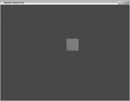
Now, drawing will occur anywhere the stencil buffer is not equal (GL_NOTEQUAL) to 0x1, which is anywhere onscreen that the spiral line is not drawn. The subsequent call to glStencilOp is optional for this example, but it tells OpenGL to leave the stencil buffer alone for all future drawing operations. Although this sample is best seen in action, Figure 3.38 shows an image of what the bounding red square looks like as it is “stenciled out.”
Figure 3.38. The bouncing red square with masking stencil pattern.
Just as with the depth buffer, you can also mask out writes to the stencil buffer by using the function glStencilMask:
void glStencilMask(GLboolean mask);
Setting the mask to false does not disable stencil test operations but does prevent any operation from writing values into the stencil buffer.
Summary
We covered a lot of ground in this chapter. At this point, you can create your 3D space for rendering, and you know how to draw everything from points and lines to complex polygons. We also showed you how to assemble these two-dimensional primitives as the surface of three-dimensional objects.
You also learned about some of the other buffers that OpenGL renders into besides the color buffer. As we move forward throughout the book, we will use the depth and stencil buffers for many other techniques and special effects. In Chapter 6, you will learn about yet another OpenGL buffer, the Accumulation buffer. You’ll see later that all these buffers working together can create some outstanding and very realistic 3D graphics.
We encourage you to experiment with what you have learned in this chapter. Use your imagination and create some of your own 3D objects before moving on to the rest of the book. You’ll then have some personal samples to work with and enhance as you learn and explore new techniques throughout the book.