
Chapter 5. Color, Materials, and Lighting: The Basics
WHAT YOU’LL LEARN IN THIS CHAPTER:

This is the chapter where 3D graphics really start to look interesting (unless you really dig wireframe models!), and it only gets better from here. You’ve been learning OpenGL from the ground up—how to put programs together and then how to assemble objects from primitives and manipulate them in 3D space. Until now, we’ve been laying the foundation, and you still can’t tell what the house is going to look like! To recoin a phrase, “Where’s the beef?”
To put it succinctly, the beef starts here. For most of the rest of this book, science takes a back seat and magic rules. According to Arthur C. Clarke, “Any sufficiently advanced technology is indistinguishable from magic.” Of course, there is no real magic involved in color and lighting, but it sure can seem that way at times. If you want to dig into the “sufficiently advanced technology” (mathematics), see Appendix A, “Further Reading/References.”
Another name for this chapter might be “Adding Realism to Your Scenes.” You see, there is more to an object’s color in the real world than just what color we might tell OpenGL to make it. In addition to having a color, objects can appear shiny or dull or can even glow with their own light. An object’s apparent color varies with bright or dim lighting, and even the color of the light hitting an object makes a difference. An illuminated object can even be shaded across its surface when lit or viewed from an angle.
What Is Color?
First, let’s talk a little bit about color itself. How is a color made in nature, and how do we see colors? Understanding color theory and how the human eye sees a color scene will lend some insight into how you create a color programmatically. (If color theory is old hat to you, you can probably skip this section.)
Light as a Wave
Color is simply a wavelength of light that is visible to the human eye. If you had any physics classes in school, you might remember something about light being both a wave and a particle. It is modeled as a wave that travels through space much like a ripple through a pond, and it is modeled as a particle, such as a raindrop falling to the ground. If this concept seems confusing, you know why most people don’t study quantum mechanics!
The light you see from nearly any given source is actually a mixture of many different kinds of light. These kinds of light are identified by their wavelengths. The wavelength of light is measured as the distance between the peaks of the light wave, as illustrated in Figure 5.1.
Figure 5.1. How a wavelength of light is measured.

Wavelengths of visible light range from 390 nanometers (one billionth of a meter) for violet light to 720 nanometers for red light; this range is commonly called the visible spectrum. You’ve undoubtedly heard the terms ultraviolet and infrared; they represent light not visible to the naked eye, lying beyond the ends of the spectrum. You will recognize the spectrum as containing all the colors of the rainbow (see Figure 5.2).
Figure 5.2. The spectrum of visible light.

Light as a Particle
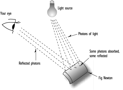
“Okay, Mr. Smart Brain,” you might ask. “If color is a wavelength of light and the only visible light is in this ‘rainbow’ thing, where is the brown for my Fig Newtons or the black for my coffee or even the white of this page?” We begin answering that question by telling you that black is not a color, nor is white. Actually, black is the absence of color, and white is an even combination of all the colors at once. That is, a white object reflects all wavelengths of colors evenly, and a black object absorbs all wavelengths evenly.
As for the brown of those fig bars and the many other colors that you see, they are indeed colors. Actually, at the physical level, they are composite colors. They are made of varying amounts of the “pure” colors found in the spectrum. To understand how this concept works, think of light as a particle. Any given object when illuminated by a light source is struck by “billions and billions” (my apologies to the late Carl Sagan) of photons, or tiny light particles. Remembering our physics mumbo jumbo, each of these photons is also a wave, which has a wavelength and thus a specific color in the spectrum.
All physical objects consist of atoms. The reflection of photons from an object depends on the kinds of atoms, the number of each kind, and the arrangement of atoms (and their electrons) in the object. Some photons are reflected and some are absorbed (the absorbed photons are usually converted to heat), and any given material or mixture of materials (such as your fig bar) reflects more of some wavelengths than others. Figure 5.3 illustrates this principle.
Figure 5.3. An object reflects some photons and absorbs others.
Your Personal Photon Detector
The reflected light from your fig bar, when seen by your eye, is interpreted as color. The billions of photons enter your eye and are focused onto the back of your eye, where your retina acts as sort of a photographic plate. The retina’s millions of cone cells are excited when struck by the photons, and this causes neural energy to travel to your brain, which interprets the information as light and color. The more photons that strike the cone cells, the more excited they get. This level of excitation is interpreted by your brain as the brightness of the light, which makes sense; the brighter the light, the more photons there are to strike the cone cells.
The eye has three kinds of cone cells. All of them respond to photons, but each kind responds most to a particular wavelength. One is more excited by photons that have reddish wavelengths; one, by green wavelengths; and one, by blue wavelengths. Thus, light that is composed mostly of red wavelengths excites red-sensitive cone cells more than the other cells, and your brain receives the signal that the light you are seeing is mostly reddish. You do the math: A combination of different wavelengths of various intensities will, of course, yield a mix of colors. All wavelengths equally represented thus are perceived as white, and no light of any wavelength is black.
You can see that any “color” that your eye perceives actually consists of light all over the visible spectrum. The “hardware” in your eye detects what it sees in terms of the relative concentrations and strengths of red, green, and blue light. Figure 5.4 shows how brown is composed of a photon mix of 60% red photons, 40% green photons, and 10% blue photons.
Figure 5.4. How the “color” brown is perceived by the eye.

The Computer as a Photon Generator
Now that you understand how the human eye discerns colors, it makes sense that when you want to generate a color with a computer, you do so by specifying separate intensities for the red, green, and blue components of the light. It so happens that color computer monitors are designed to produce three kinds of light (can you guess which three?), each with varying degrees of intensity. For years the CRT (Cathode Ray Tube) reigned supreme. In the back of these computer monitors is an electron gun that shoots electrons at the back of the screen. This screen contains phosphors that emit red, green, and blue light when struck by the electrons. The intensity of the light emitted varies with the intensity of the electron beam. These three color phosphors are packed closely together to make up a single physical dot on the screen (see Figure 5.5).
Figure 5.5. How a computer monitor generates colors.
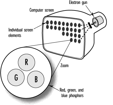
A few hold-outs still prefer the CRT technology over LCD (Liquid Crystal Display) for various reasons, such as higher refresh rate. LCDs work in a similar way by combining three colors of light, except they are solid state. Each pixel on your LCD screen has a light behind it and three very small computer-controlled polarized (red, green, and blue) filters. Basic LCD technology is based on the polarization of light, and blocking that light with the LCD material electronically. A huge technological achievement to be sure, but it still all boils down to very crowded tiny dots emitting red, green, and blue light.
You might recall that in Chapter 2, “Using OpenGL,” we explained how OpenGL defines a color exactly as intensities of red, green, and blue, with the glColor command.
PC Color Hardware
There once was a time (actually, 1982) when state-of-the-art PC graphics hardware meant the Hercules graphics card. This card could produce bitmapped images with a resolution of 720×348, and crisper text than the original IBM Monochrome Display Adapter (MDA) developed for the original IBM PC. The drawback was that each pixel had only two states: on and off. At that time, bitmapped graphics of any kind on a PC were a big deal, and you could produce some great monochrome graphics—even 3D!
Actually predating the Hercules card by one year was the Color Graphics Adapter (CGA) card. Also introduced with the first IBM PC, this card could support resolutions of 320×200 pixels and could place any 4 of 16 colors on the screen at once. A higher resolution (640×200) with 2 colors was also possible but wasn’t as effective or cost conscious as the Hercules card. (Color monitors = $$$.) CGA was puny by today’s standards; it was even outmatched by the graphics capabilities of a $200 Commodore 64 or Atari home computer at the time. Lacking adequate resolution for business graphics or even modest modeling, CGA was used primarily for simple PC games or business applications that could benefit from colored text. Generally, it was hard to make a good business justification for this more expensive hardware.
The next big breakthrough for PC graphics came in 1984 when IBM introduced the Enhanced Graphics Adapter (EGA) card. This one could do more than 25 lines of colored text in new text modes, and for graphics, it could support 640×350-pixel bitmapped graphics in 16 colors! Other technical improvements eliminated some flickering problems of the CGA ancestor and provided for better and smoother animation. Now arcade-style games, real business graphics, and even simple 3D graphics became not only possible but even reasonable on the PC. This advance was a giant move beyond CGA, but still PC graphics were in their infancy.
The last mainstream PC graphics standard set by IBM was the VGA card (which stood for Video Graphics Array rather than the commonly held Video Graphics Adapter), introduced in 1987. This card was significantly faster than the EGA; it could support 16 colors at a higher resolution (640×480) and 256 colors at a lower resolution of 320×200. These 256 colors were selected from a palette of more than 16 million possible colors. That’s when the floodgates opened for PC graphics. Near photo-realistic graphics became possible on PCs. Ray tracers, 3D games, and photo-editing software began to pop up in the PC market.
IBM, as well, had a high-end graphics card—the 8514—, introduced in 1987 for its “workstations.” This card could do 1,024×768 graphics at 256 colors, and came with a whopping one megabyte of memory! IBM thought this card would be used only by CAD and scientific applications! But one thing is certain about consumers: They always want more. It was this short-sightedness that cost IBM its role as standard setter in the PC graphics market. Other vendors began to ship “Super-VGA” cards that could display higher and higher resolutions, with more and more colors. First, we saw 800×600, then 1,024×768 and even higher, with first 256 colors, and then 32,000, and 65,000. Today, 32-bit color cards can display 16 million colors at resolutions far greater than 1,024×768. Even entry-level Windows PCs sold today can support at least 16 million colors at resolutions of 1,024×768 or more.
All this power makes for some really cool possibilities—photo-realistic 3D graphics, to name just one. When Microsoft ported OpenGL to the Windows platform, that move enabled creation of high-end graphics applications for PCs. Combine today’s fast processors with 3D-graphics accelerated graphics cards, and you can get the kind of performance possible only a few years ago on $100,000 graphics workstations—for the cost of a Wal-Mart Christmas special! Today’s typical home machines are capable of sophisticated simulations, games, and more. Already the term virtual reality has become as antiquated as those old Buck Rogers rocket ships as we begin to take advanced 3D graphics for granted.
PC Display Modes
Microsoft Windows and the Apple Macintosh revolutionized the world of PC graphics in two respects. First, they created mainstream graphical operating environments that were adopted by the business world at large and, soon thereafter, the consumer market. Second, they made PC graphics significantly easier for programmers to do. The graphics hardware was “virtualized” by display device drivers. Instead of having to write instructions directly to the video hardware, programmers today can write to a single API (such as OpenGL), and the operating system handles the specifics of talking to the hardware.
Screen Resolution
Screen resolution for today’s computers can vary from 640×480 pixels up to 1,600×1,200 or more. The lower resolutions of, say, 640×480 are considered adequate for some graphics display tasks; people with eye problems often run at the lower resolutions, but on a large monitor or display. You must always take into account the size of the window with the clipping volume and viewport settings (see Chapter 2). By scaling the size of the drawing to the size of the window, you can easily account for the various resolutions and window size combinations that can occur. Well-written graphics applications display the same approximate image regardless of screen resolution. The user should automatically be able to see more and sharper details as the resolution increases.
Color Depth
If an increase in screen resolution or in the number of available drawing pixels in turn increases the detail and sharpness of the image, so too should an increase in available colors improve the clarity of the resulting image. An image displayed on a computer that can display millions of colors should look remarkably better than the same image displayed with only 16 colors.
Bang the Rocks Together!
The most primitive display modes you may ever encounter are the 4-bit (16-color) and 8-bit (256-color) modes. These modes do rarely show up, but only as the base display mode when you first install an operating system without any specific graphics card drivers. At one time, these depths were the “new hotness,” but these modes are useless by today’s standards for graphics applications and can be safely ignored.
Going Deeper
Typical consumer graphics hardware today comes in three flavors: 16, 24, and 32 bits per pixel. The 16-bit display modes are available on many shipping graphics cards today, but are rarely used on purpose. This mode supports 65,536 different colors, and consumes less memory for the color buffer than the higher bit depth modes. Many graphics applications have very noticeable visual artifacts (usually in color gradations) at this color depth. The 24- and 32-bit display modes support 8 bits of color per color component, allowing more than 16 million colors onscreen at a time.
Nearly all 3D graphics hardware today supports 32-bit color mode. This allows for 8 bits per RGBA color channel. Visually, there is no real difference between 24- and 32-bit display modes. A graphics card that reserves 32 bits per pixel does so for one of two reasons. First, most memory architectures perform faster with each pixel occupying exactly 4 bytes instead of 3. Second, the extra 8 bits per pixel can be used to store an alpha value in the color buffer. This alpha value can be used for some graphics operations. You’ll learn more about uses for alpha in the next chapter.
In Chapter 18, “Advanced Buffers,” you’ll learn about OpenGL’s support for the most cutting-edge color technology: floating-point color buffers.
Using Color in OpenGL
You now know that OpenGL specifies an exact color as separate intensities of red, green, and blue components. You also know that modern PC hardware might be able to display nearly all these combinations or only a very few. How, then, do we specify a desired color in terms of these red, green, and blue components?
The Color Cube
Because a color is specified by three positive color values, we can model the available colors as a volume that we call the RGB colorspace. Figure 5.6 shows what this colorspace looks like at the origin with red, green, and blue as the axes. The red, green, and blue coordinates are specified just like x, y, and z coordinates. At the origin (0,0,0), the relative intensity of each component is zero, and the resulting color is black. The maximum available on the PC for storage information is 24 bits, so with 8 bits for each component, let’s say that a value of 255 along the axis represents full saturation of that component. We then end up with a cube measuring 255 on each side. The corner directly opposite black, where the concentrations are (0,0,0), is white, with relative concentrations of (255,255,255). At full saturation (255) from the origin along each axis lie the pure colors of red, green, and blue.
Figure 5.6. The origin of RGB colorspace.

This “color cube” (see Figure 5.7) contains all the possible colors, either on the surface of the cube or within the interior of the cube. For example, all possible shades of gray between black and white lie internally on the diagonal line between the corner at (0,0,0) and the corner at (255,255,255).
Figure 5.7. The RGB colorspace.

Figure 5.8 shows the smoothly shaded color cube produced by a sample program from this chapter, CCUBE. The surface of this cube shows the color variations from black on one corner to white on the opposite corner. Red, green, and blue are present on their corners 255 units from black. Additionally, the colors yellow, cyan, and magenta have corners showing the combination of the other three primary colors. You can also spin the color cube around to examine all its sides by pressing the arrow keys.
Figure 5.8. The output from CCUBE is this color cube.

Setting the Drawing Color
Let’s briefly review the glColor function. It is prototyped as follows:
void glColor<x><t>(red, green, blue, alpha);
In the function name, the <x> represents the number of arguments; it might be 3 for three arguments of red, green, and blue or 4 for four arguments to include the alpha component. The alpha component specifies the translucency of the color and is covered in more detail in the next chapter. For now, just use a three-argument version of the function.
The <t> in the function name specifies the argument’s data type and can be b, d, f, i, s, ub, ui, or us, for byte, double, float, integer, short, unsigned byte, unsigned integer, and unsigned short data types, respectively. Another version of the function has a v appended to the end; this version takes an array that contains the arguments (the v stands for vectored). In Appendix C, “API Reference,” you will find an entry with more details on the glColor function.
Most OpenGL programs that you’ll see use glColor3f and specify the intensity of each component as 0.0 for none or 1.0 for full intensity. However, it might be easier, if you have Windows programming experience, to use the glColor3ub version of the function. This version takes three unsigned bytes, from 0 to 255, to specify the intensities of red, green, and blue. Using this version of the function is like using the Windows RGB macro to specify a color:
glColor3ub(0,255,128) = RGB(0,255,128)
In fact, this approach might make it easier for you to match your OpenGL colors to existing RGB colors used by your program for other non-OpenGL drawing tasks. However, we should say that, internally, OpenGL represents color values as floating-point values, and you may incur some performance penalties due to the constant conversion to floats that must take place at runtime. It is also possible that in the future, higher resolution color buffers may evolve (in fact, floating-point color buffers are already starting to appear), and your color values specified as floats will be more faithfully represented by the color hardware.
Shading
Our previous working definition for glColor was that this function sets the current drawing color, and all objects drawn after this command have the last color specified. After discussing the OpenGL drawing primitives in a preceding chapter, we can now expand this definition as follows: The glColor function sets the current color that is used for all vertices drawn after the command. So far, all our examples have drawn wireframe objects or solid objects with each face a different solid color. If we specify a different color for each vertex of a primitive (point, line, or polygon), what color is the interior?
Let’s answer this question first regarding points. A point has only one vertex, and whatever color you specify for that vertex is the resulting color for that point. Easy enough.
A line, however, has two vertices, and each can be set to a different color. The color of the line depends on the shading model. Shading is simply defined as the smooth transition from one color to the next. Any two points in the RGB colorspace (refer to Figure 5.7) can be connected by a straight line.
Smooth shading causes the colors along the line to vary as they do through the color cube from one color point to the other. Figure 5.9 shows the color cube with the black and white corners identified. Below it is a line with two vertices, one black and one white. The colors selected along the length of the line match the colors along the straight line in the color cube, from the black to the white corners. This results in a line that progresses from black through lighter shades of gray and eventually to white.
Figure 5.9. How a line is shaded from black to white.

You can do shading mathematically by finding the equation of the line connecting two points in the three-dimensional RGB colorspace. Then you can simply loop through from one end of the line to the other, retrieving coordinates along the way to provide the color of each pixel on the screen. Many good books on computer graphics explain the algorithm to accomplish this effect, scale your color line to the physical line on the screen, and so on. Fortunately, OpenGL does all this work for you!
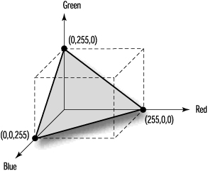
The shading exercise becomes slightly more complex for polygons. A triangle, for instance, can also be represented as a plane within the color cube. Figure 5.10 shows a triangle with each vertex at full saturation for the red, green, and blue color components. The code to display this triangle is shown in Listing 5.1 and in the sample program titled TRIANGLE.
Figure 5.10. A triangle in RGB colorspace.
Listing 5.1. Drawing a Smooth-Shaded Triangle with Red, Green, and Blue Corners
// Enable smooth shading
glShadeModel(GL_SMOOTH);
// Draw the triangle
glBegin(GL_TRIANGLES);
// Red Apex
glColor3ub((GLubyte)255,(GLubyte)0,(GLubyte)0);
glVertex3f(0.0f,200.0f,0.0f);
// Green on the right bottom corner
glColor3ub((GLubyte)0,(GLubyte)255,(GLubyte)0);
glVertex3f(200.0f,-70.0f,0.0f);
// Blue on the left bottom corner
glColor3ub((GLubyte)0,(GLubyte)0,(GLubyte)255);
glVertex3f(-200.0f, -70.0f, 0.0f);
glEnd();
Setting the Shading Model
The first line of Listing 5.1 actually sets the shading model OpenGL uses to do smooth shading—the model we have been discussing. This is the default shading model, but it’s a good idea to call this function anyway to ensure that your program is operating the way you intended.
The other shading model that can be specified with glShadeModel is GL_FLAT for flat shading. Flat shading means that no shading calculations are performed on the interior of primitives. Generally, with flat shading, the color of the primitive’s interior is the color that was specified for the last vertex. The only exception is for a GL_POLYGON primitive, in which case the color is that of the first vertex.
Next, the code in Listing 5.1 sets the top of the triangle to be pure red, the lower-right corner to be green, and the remaining lower-left corner to be blue. Because smooth shading is specified, the interior of the triangle is shaded to provide a smooth transition between each corner.
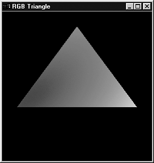
The output from the TRIANGLE program is shown in Figure 5.11. This output represents the plane shown graphically in Figure 5.10.
Figure 5.11. The output from the TRIANGLE program.
Polygons, more complex than triangles, can also have different colors specified for each vertex. In these instances, the underlying logic for shading can become more intricate. Fortunately, you never have to worry about it with OpenGL. No matter how complex your polygon, OpenGL successfully shades the interior points between each vertex.
Color in the Real World
Real objects don’t appear in a solid or shaded color based solely on their RGB values. Figure 5.12 shows the output from the program titled JET from the sample code for this chapter. It’s a simple jet airplane, hand plotted with triangles using only the methods covered so far in this book. As usual, JET and the other example programs in this chapter allow you to spin the object around by using the arrow keys to better see the effects.
Figure 5.12. A simple jet built by setting a different color for each triangle.

The selection of colors is meant to highlight the three-dimensional structure of the jet. Aside from the crude assemblage of triangles, however, you can see that the jet looks hardly anything like a real object. Suppose you constructed a model of this airplane and painted each flat surface the colors represented. The model would still appear glossy or flat depending on the kind of paint used, and the color of each flat surface would vary with the angle of your view and any sources of light.
OpenGL does a reasonably good job of approximating the real world in terms of lighting conditions. To do so, it uses a simple and intuitive lighting model that isn’t necessarily based on the physics of real world light. In the OpenGL lighting model, unless an object emits its own light, it is illuminated by three kinds of light: ambient, diffuse, and specular. In the real world, there is of course no such thing. However, for our abstraction of lighting, these three kinds of light allow us to simulate and control the three main kinds of effects that light has when shining on materials.
Ambient Light
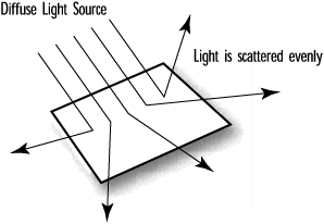
Ambient light doesn’t come from any particular direction. It has an original source somewhere, but the rays of light have bounced around the room or scene and become directionless. Objects illuminated by ambient light are evenly lit on all surfaces in all directions. You can think of all previous examples in this book as being lit by a bright ambient light because the objects were always visible and evenly colored (or shaded) regardless of their rotation or viewing angle. Figure 5.13 shows an object illuminated by ambient light. You can think of ambient light as a global “brightening” factor applied per light source. In OpenGL, this lighting component really approximates scattered light in the environment that originates from the light source.
Figure 5.13. An object illuminated purely by ambient light.

Diffuse Light
The diffuse part of an OpenGL light is the directional component that appears to come from a particular direction and is reflected off a surface with an intensity proportional to the angle at which the light rays strike the surface. Thus, the object surface is brighter if the light is pointed directly at the surface than if the light grazes the surface from a greater angle. Good examples of diffuse light sources include a lamp, candle, or sunlight streaming in a side window at noon. Essentially, it is the diffuse component of a light source that produces the shading (or change in color) across a lit object’s surface. In Figure 5.14, the object is illuminated by a diffuse light source.
Figure 5.14. An object illuminated by a purely diffuse light source.
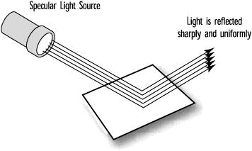
Specular Light
Like diffuse light, specular light is a highly directional property, but it interacts more sharply with the surface and in a particular direction. A highly specular light (really a material property in the real world) tends to cause a bright spot on the surface it shines on, which is called the specular highlight. Because of its highly directional nature, it is even possible that depending on a viewer’s position, the specular highlight may not even be visible. A spotlight and the sun are good examples of sources that produce strong specular highlights. Figure 5.15 shows an object illuminated by a purely specular light source.
Figure 5.15. An object illuminated by a purely specular light source.
Putting It All Together
No single light source is composed entirely of any of the three types of light just described. Rather, it is made up of varying intensities of each. For example, a red laser beam in a lab is composed of almost a pure-red specular component producing a very bright spot where it strikes any object. However, smoke or dust particles scatter the beam all over the room, giving it a very small ambient component. This would produce a slight red hue on other objects in the room. If the beam strikes a surface at a glancing blow, a very small diffuse shading component may be seen across the surface it illuminates (although in this case it would be largely overpowered by the specular highlight).
Thus, a light source in a scene is said to be composed of three lighting components: ambient, diffuse, and specular. Just like the components of a color, each lighting component is defined with an RGBA value that describes the relative intensities of red, green, and blue light that make up that component (for the purposes of light color, the alpha value is ignored). For example, our red laser light might be described by the component values in Table 5.1.
Table 5.1. Color and Light Distribution for a Red Laser Light Source

Note that the red laser beam has no green or blue light. Also, note that specular, diffuse, and ambient light can each range in intensity from 0.0 to 1.0. You could interpret this table as saying that the red laser light in some scenes has a very high specular component, a small diffuse component, and a very small ambient component. Wherever it shines, you are probably going to see a reddish spot. Also, because of conditions in the room, the ambient component—likely due to smoke or dust particles in the air—scatters a tiny bit of light all about the room.
Materials in the Real World
Light is only part of the equation. In the real world, objects do have a color of their own. Earlier in this chapter, we described the color of an object as defined by its reflected wavelengths of light. A blue ball reflects mostly blue photons and absorbs most others. This assumes that the light shining on the ball has blue photons in it to be reflected and detected by the observer. Generally, most scenes in the real world are illuminated by a white light containing an even mixture of all the colors. Under white light, therefore, most objects appear in their proper or “natural” colors. However, this is not always so; put the blue ball in a dark room with only a yellow light, and the ball appears black to the viewer because all the yellow light is absorbed and there is no blue to be reflected.
Material Properties
When we use lighting, we do not describe polygons as having a particular color, but rather as consisting of materials that have certain reflective properties. Instead of saying that a polygon is red, we say that the polygon is made of a material that reflects mostly red light. We are still saying that the surface is red, but now we must also specify the material’s reflective properties for ambient, diffuse, and specular light sources. A material might be shiny and reflect specular light very well, while absorbing most of the ambient or diffuse light. Conversely, a flat colored object might absorb all specular light and not look shiny under any circumstances. Another property to be specified is the emission property for objects that emit their own light, such as taillights or glow-in-the-dark watches.
Adding Light to Materials
Setting lighting and material properties to achieve the desired effect takes some practice. There are no color cubes or rules of thumb to give you quick and easy answers. This is the point at which analysis gives way to art, and science yields to magic. When drawing an object, OpenGL decides which color to use for each pixel in the object. That object has reflective “colors,” and the light source has “colors” of its own. How does OpenGL determine which colors to use? Understanding these principles is not difficult, but it does take some simple grade-school multiplication. (See, that teacher told you you’d need it one day!)
Each vertex of your primitives is assigned an RGB color value based on the net effect of the ambient, diffuse, and specular illumination multiplied by the ambient, diffuse, and specular reflectance of the material properties. Because you make use of smooth shading between the vertices, the illusion of illumination is achieved.
Calculating Ambient Light Effects
To calculate ambient light effects, you first need to put away the notion of color and instead think only in terms of red, green, and blue intensities. For an ambient light source of half-intensity red, green, and blue components, you have an RGB value for that source of (0.5, 0.5, 0.5). If this ambient light illuminates an object with ambient reflective properties specified in RGB terms of (0.5, 1.0, 0.5), the net “color” component from the ambient light is
(0.5 * 0.5, 0.5 * 1.0, 0.5 * 0.5) = (0.25, 0.5, 0.25)
This is the result of multiplying each of the ambient light source terms by each of the ambient material property terms (see Figure 5.16).
Figure 5.16. Calculating the ambient color component of an object.

Thus, the material color components actually determine the percentage of incident light that is reflected. In our example, the ambient light had a red component that was at one-half intensity, and the material ambient property of 0.5 specified that one-half of that one-half intensity light was reflected. Half of a half is a fourth, or 0.25.
Diffuse and Specular Effects
Calculating ambient light is as simple as it gets. Diffuse light also has RGB intensities that interact in the same way with material properties. However, diffuse light is directional, and the intensity at the surface of the object varies depending on the angle between the surface and the light source, the distance to the light source, any attenuation factors (whether it is foggy between the light and the surface), and so on. The same goes for specular light sources and intensities. The net effect in terms of RGB values is figured the same way as for ambient light, with the intensity of the light source (adjusted for the angle of incidence) being multiplied by the material reflectance. Finally, all three RGB terms are added to yield a final color for the object. If any single color component is greater than 1.0, it is clamped to that value. (You can’t get more intense than full intensity!)
Generally, the ambient and diffuse components of light sources and materials are the same and have the greatest effect in determining the color of the object. Specular light and material properties tend to be light gray or white. The specular component depends significantly on the angle of incidence, and specular highlights on an object are usually set to white.
Adding Light to a Scene
This text might seem like a lot of theory to digest all of a sudden. Let’s slow down and start exploring some examples of the OpenGL code needed for lighting; this exploration will also help reinforce what you’ve just learned. We demonstrate some additional features and requirements of lighting in OpenGL. The next few examples build on our JET program. The initial version contains no lighting code and just draws triangles with hidden surface elimination (depth testing) enabled. When we’re done, the jet’s metallic surface will glisten in the sunlight as you rotate it with the arrow keys.
Enabling the Lighting
To tell OpenGL to use lighting calculations, call glEnable with the GL_LIGHTING parameter:
glEnable(GL_LIGHTING);
This call alone tells OpenGL to use material properties and lighting parameters in determining the color for each vertex in your scene. However, without any specified material properties or lighting parameters, your object remains dark and unlit, as shown in Figure 5.17. Look at the code for any of the JET-based sample programs, and you can see that we have called the function SetupRC right after creating the rendering context. This is the place where we do any initialization of lighting parameters.
Figure 5.17. An unlit jet reflects no light.

Setting Up Cosmic Background Radiation
There is a global light source in OpenGL that emits only ambient light. I call this the Cosmic Background Radiation—a term borrowed from the Big Bang theory—because it’s a light source that shines evenly in all directions. This global ambient illumination is a zero-cost way to add a simple offset to the results of OpenGL lighting calculations. This can be useful, for example, to illuminate the back sides of objects that are not being illuminated directly by a light source. If your lit scene appears too dark, you can monkey with this ambient light until you get the levels you want.
This global ambient light is set in the OpenGL light model, which can be modified with the glLightModel function.
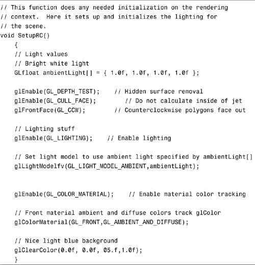
The first lighting parameter used in our next example (the AMBIENT program) is GL_LIGHT_MODEL_AMBIENT. It lets you specify a global ambient light that illuminates all objects evenly from all sides. The following code specifies a bright white light:
// Bright white light - full intensity RGB values
GLfloat ambientLight[] = { 1.0f, 1.0f, 1.0f, 1.0f };
// Enable lighting
glEnable(GL_LIGHTING);
// Set light model to use ambient light specified by ambientLight[]
glLightModelfv(GL_LIGHT_MODEL_AMBIENT,ambientLight);
The variation of glLightModel shown here, glLightModelfv, takes as its first parameter the lighting model parameter being modified or set and then an array of the RGBA values that make up the light. The default RGBA values of this global ambient light are (0.2, 0.2, 0.2, 1.0), which is fairly dim. Other lighting model parameters allow you to determine whether the front, back, or both sides of polygons are illuminated and how the calculation of specular lighting angles is performed. See the reference section in Appendix C for more information on these parameters.
Setting Material Properties
Now that we have an ambient light source, we need to set some material properties so that our polygons reflect light and we can see our jet. There are two ways to set material properties. The first is to use the function glMaterial before specifying each polygon or set of polygons. Examine the following code fragment:
Glfloat gray[] = { 0.75f, 0.75f, 0.75f, 1.0f };
...
...
glMaterialfv(GL_FRONT, GL_AMBIENT_AND_DIFFUSE, gray);
glBegin(GL_TRIANGLES);
glVertex3f(-15.0f,0.0f,30.0f);
glVertex3f(0.0f, 15.0f, 30.0f);
glVertex3f(0.0f, 0.0f, -56.0f);
glEnd();
The first parameter to glMaterialfv specifies whether the front, back, or both (GL_FRONT, GL_BACK, or GL_FRONT_AND_BACK) take on the material properties specified. The second parameter tells which properties are being set; in this instance, both the ambient and diffuse reflectances are set to the same values. The final parameter is an array containing the RGBA values that make up these properties. All primitives specified after the glMaterial call are affected by the last values set, until another call to glMaterial is made.
Under most circumstances, the ambient and diffuse components are the same, and unless you want specular highlights (sparkling, shiny spots), you don’t need to define specular reflective properties. Even so, it would still be quite tedious if we had to define an array for every color in our object and call glMaterial before each polygon or group of polygons.
Now we are ready for the second and preferred way of setting material properties, called color tracking. With color tracking, you can tell OpenGL to set material properties by only calling glColor. To enable color tracking, call glEnable with the GL_COLOR_MATERIAL parameter:
glEnable(GL_COLOR_MATERIAL);
Then the function glColorMaterial specifies the material parameters that follow the values set by glColor. For example, to set the ambient and diffuse properties of the fronts of polygons to track the colors set by glColor, call
glColorMaterial(GL_FRONT,GL_AMBIENT_AND_DIFFUSE);
The earlier code fragment setting material properties would then be as follows. This approach looks like more code, but it actually saves many lines of code and executes faster as the number of different colored polygons grows:
// Enable color tracking
glEnable(GL_COLOR_MATERIAL);
// Front material ambient and diffuse colors track glColor
glColorMaterial(GL_FRONT,GL_AMBIENT_AND_DIFFUSE);
...
...
glcolor3f(0.75f, 0.75f, 0.75f);
glBegin(GL_TRIANGLES);
glVertex3f(-15.0f,0.0f,30.0f);
glVertex3f(0.0f, 15.0f, 30.0f);
glVertex3f(0.0f, 0.0f, -56.0f);
glEnd();
Listing 5.2 contains the code we add with the SetupRC function to our jet example to set up a bright ambient light source and to set the material properties that allow the object to reflect light and be seen. We have also changed the colors of the jet so that each section rather than each polygon is a different color. The final output, shown in Figure 5.18, is not much different from the image before we had lighting. However, if we reduce the ambient light by half, we get the image shown in Figure 5.19. To reduce it by half, we set the ambient light RGBA values to the following:
GLfloat ambientLight[] = { 0.5f, 0.5f, 0.5f, 1.0f };
Figure 5.18. The output from the completed AMBIENT sample program.

Figure 5.19. The output from the AMBIENT program when the light source is cut in half.

You can see how we might reduce the ambient light in a scene to produce a dimmer image. This capability is useful for simulations in which dusk approaches gradually or when a more direct light source is blocked, as when an object is in the shadow of another, larger object.
Listing 5.2. Setup for Ambient Lighting Conditions
Using a Light Source
Manipulating the ambient light has its uses, but for most applications attempting to model the real world, you must specify one or more specific sources of light. In addition to their intensities and colors, these sources have a location and/or a direction. The placement of these lights can dramatically affect the appearance of your scene.
OpenGL supports at least eight independent light sources located anywhere in your scene or out of the viewing volume. You can locate a light source an infinite distance away and make its light rays parallel or make it a nearby light source radiating outward. You can also specify a spotlight with a specific cone of light radiating from it, as well as manipulate its characteristics.
Which Way Is Up?
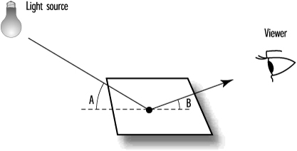
When you specify a light source, you tell OpenGL where it is and in which direction it’s shining. Often, the light source shines in all directions, but it can be directional. Either way, for any object you draw, the rays of light from any source (other than a pure ambient source) strike the surface of the polygons that make up the object at an angle. Of course, in the case of a directional light, the surfaces of all polygons might not necessarily be illuminated. To calculate the shading effects across the surface of the polygons, OpenGL must be able to calculate the angle.
In Figure 5.20, a polygon (a square) is being struck by a ray of light from some source. The ray makes an angle (A) with the plane as it strikes the surface. The light is then reflected at an angle (B) toward the viewer (or you wouldn’t see it). These angles are used in conjunction with the lighting and material properties we have discussed thus far to calculate the apparent color of that location. It happens by design that the locations used by OpenGL are the vertices of the polygon. Because OpenGL calculates the apparent colors for each vertex and then does smooth shading between them, the illusion of lighting is created. Magic!
Figure 5.20. Light is reflected off objects at specific angles.
From a programming standpoint, these lighting calculations present a slight conceptual difficulty. Each polygon is created as a set of vertices, which are nothing more than points. Each vertex is then struck by a ray of light at some angle. How then do you (or OpenGL) calculate the angle between a point and a line (the ray of light)? Of course, you can’t geometrically find the angle between a single point and a line in 3D space because there are an infinite number of possibilities. Therefore, you must associate with each vertex some piece of information that denotes a direction upward from the vertex and away from the surface of the primitive.
Surface Normals
A line from the vertex in the upward direction starts in some imaginary plane (or your polygon) at a right angle. This line is called a normal vector. The term normal vector might sound like something the Star Trek crew members toss around, but it just means a line perpendicular to a real or imaginary surface. A vector is a line pointed in some direction, and the word normal is just another way for eggheads to say perpendicular (intersecting at a 90° angle). As if the word perpendicular weren’t bad enough! Therefore, a normal vector is a line pointed in a direction that is at a 90° angle to the surface of your polygon. Figure 5.21 presents examples of 2D and 3D normal vectors.
Figure 5.21. A 2D and a 3D normal vector.

You might already be asking why we must specify a normal vector for each vertex. Why can’t we just specify a single normal for a polygon and use it for each vertex? We can—and for our first few examples, we do. However, sometimes you don’t want each normal to be exactly perpendicular to the surface of the polygon. You may have noticed that many surfaces are not flat! You can approximate these surfaces with flat, polygonal sections, but you end up with a jagged or multifaceted surface. Later, we discuss a technique to produce the illusion of smooth curves with flat polygons by “tweaking” surface normals (more magic!). But first things first...
Specifying a Normal
To see how we specify a normal for a vertex, let’s look at Figure 5.22—a plane floating above the xz plane in 3D space. We’ve made this illustration simple to demonstrate the concept. Notice the line through the vertex (1,1,0) that is perpendicular to the plane. If we select any point on this line, say (1,10,0), the line from the first point (1,1,0) to the second point (1,10,0) is our normal vector. The second point specified actually indicates that the direction from the vertex is up in the y direction. This convention is also used to indicate the front and back sides of polygons, as the vector travels up and away from the front surface.
Figure 5.22. A normal vector traveling perpendicular from the surface.

You can see that this second point is the number of units in the x, y, and z directions for some point on the normal vector away from the vertex. Rather than specify two points for each normal vector, we can subtract the vertex from the second point on the normal, yielding a single coordinate triplet that indicates the x, y, and z steps away from the vertex. For our example, this is
(1,10,0) – (1,1,0) = (1 – 1, 10 – 1, 0) = (0,9,0)
Here’s another way of looking at this example: If the vertex were translated to the origin, the point specified by subtracting the two original points would still specify the direction pointing away and at a 90° angle from the surface. Figure 5.23 shows the newly translated normal vector.
Figure 5.23. The newly translated normal vector.

The vector is a directional quantity that tells OpenGL which direction the vertices (or polygon) face. This next code segment shows a normal vector being specified for one of the triangles in the JET sample program:
glBegin(GL_TRIANGLES);
glNormal3f(0.0f, -1.0f, 0.0f);
glVertex3f(0.0f, 0.0f, 60.0f);
glVertex3f(-15.0f, 0.0f, 30.0f);
glVertex3f(15.0f,0.0f,30.0f);
glEnd();
The function glNormal3f takes the coordinate triplet that specifies a normal vector pointing in the direction perpendicular to the surface of this triangle. In this example, the normals for all three vertices have the same direction, which is down the negative y-axis. This is a simple example because the triangle is lying flat in the xz plane, and it actually represents a bottom section of the jet. You’ll see later that often we want to specify a different normal for each vertex.
The prospect of specifying a normal for every vertex or polygon in your drawing might seem daunting, especially because few surfaces lie cleanly in one of the major planes. Never fear! Shortly we’ll present a reusable function that you can call again and again to calculate your normals for you.
Unit Normals
As OpenGL does its magic, all surface normals must eventually be converted to unit normals. A unit normal is just a normal vector that has a length of 1. The normal in Figure 5.23 has a length of 9. You can find the length of any normal by squaring each component, adding them together, and taking the square root. Divide each component of the normal by the length, and you get a vector pointed in exactly the same direction, but only 1 unit long. In this case, our new normal vector is specified as (0,1,0). This is called normalization. Thus, for lighting calculations, all normal vectors must be normalized. Talk about jargon!
You can tell OpenGL to convert your normals to unit normals automatically, by enabling normalization with glEnable and a parameter of GL_NORMALIZE:
glEnable(GL_NORMALIZE);
This approach does, however, have performance penalties on some implementations. It’s far better to calculate your normals ahead of time as unit normals instead of relying on OpenGL to perform this task for you.
You should note that calls to the glScale transformation function also scale the length of your normals. If you use glScale and lighting, you can obtain undesired results from your OpenGL lighting. If you have specified unit normals for all your geometry and used a constant scaling factor with glScale (all geometry is scaled by the same amount), an alternative to GL_NORMALIZE (available in OpenGL 1.2 and later) is GL_RESCALE_NORMALS. You enable this parameter with a call such as
glEnable(GL_RESCALE_NORMALS);
This call tells OpenGL that your normals are not unit length, but they can all be scaled by the same amount to make them unit length. OpenGL figures this out by examining the modelview matrix. The result is fewer mathematical operations per vertex than are otherwise required.
Because it is better to give OpenGL unit normals to begin with, the math3d library comes with a function that will take any normal vector and “normalize” it for you:
void m3dNormalizeVector(M3DVector3f vNormal);
Finding a Normal
Figure 5.24 presents another polygon that is not simply lying in one of the axis planes. The normal vector pointing away from this surface is more difficult to guess, so we need an easy way to calculate the normal for any arbitrary polygon in 3D coordinates.
Figure 5.24. A nontrivial normal problem.

You can easily calculate the normal vector for any polygon by taking three points that lie in the plane of that polygon. Figure 5.25 shows three points—P1, P2, and P3—that you can use to define two vectors: vector V1 from P1 to P2, and vector V2 from P1 to P3. Mathematically, two vectors in three-dimensional space define a plane. (Your original polygon lies in this plane.) If you take the cross product of those two vectors (written mathematically as V1 X V2), the resulting vector is perpendicular to that plane. Figure 5.26 shows the vector V3 derived by taking the cross product of V1 and V2. Be careful to get the order correct. Cross products are not like multiplication of scalar values. The vector produced by V1 X V2 points in the opposite direction of a vector produced by V2 X V1.
Figure 5.25. Two vectors defined by three points on a plane.

Figure 5.26. A normal vector as the cross product of two vectors.

Again, because this is such a useful and often-used method, the math3d library contains a function that calculates a normal vector based on three points on a polygon:
void m3dFindNormal(M3DVector3f vNormal, const M3DVector3f vP1,
const M3DVector3f vP2, const M3DVector3f vP3);
To use this function, pass it a vector to store the normal, and three vectors (each just an array of three floats) from your polygon or triangle (specified in counterclockwise winding order). Note that this returned normal vector is not necessarily unit length (normalized).
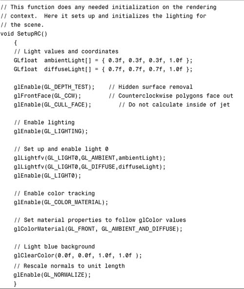
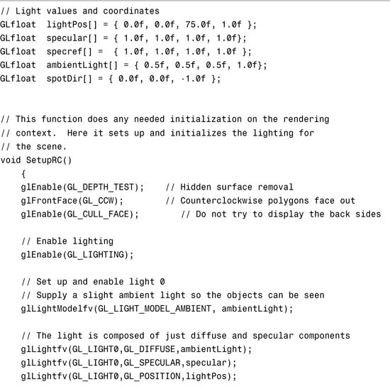
Setting Up a Source
Now that you understand the requirements of setting up your polygons to receive and interact with a light source, it’s time to turn on the lights! Listing 5.3 shows the SetupRC function from the sample program LITJET. Part of the setup process for this sample program creates a light source and places it to the upper left, slightly behind the viewer. The light source GL_LIGHT0 has its ambient and diffuse components set to the intensities specified by the arrays ambientLight[] and diffuseLight[]. This results in a moderate white light source:
GLfloat ambientLight[] = { 0.3f, 0.3f, 0.3f, 1.0f };
GLfloat diffuseLight[] = { 0.7f, 0.7f, 0.7f, 1.0f };
...
...
// Set up and enable light 0
glLightfv(GL_LIGHT0,GL_AMBIENT,ambientLight);
glLightfv(GL_LIGHT0,GL_DIFFUSE,diffuseLight);
Finally, the light source GL_LIGHT0 is enabled:
glEnable(GL_LIGHT0);
The light is positioned by this code, located in the ChangeSize function:
GLfloat lightPos[] = { -50.f, 50.0f, 100.0f, 1.0f };
...
...
glLightfv(GL_LIGHT0,GL_POSITION,lightPos);
Here, lightPos[] contains the position of the light. The last value in this array is 1.0, which specifies that the designated coordinates are the position of the light source. If the last value in the array is 0.0, it indicates that the light is an infinite distance away along the vector specified by this array. We’ll touch more on this issue later. Lights are like geometric objects in that they can be moved around by the modelview matrix. By placing the light’s position when the viewing transformation is performed, we ensure that the light is in the proper location regardless of how we transform the geometry.
Listing 5.3. Light and Rendering Context Setup for LITJET
Setting the Material Properties
Notice in Listing 5.3 that color tracking is enabled, and the properties to be tracked are the ambient and diffuse reflective properties for the front surface of the polygons. This is just as it was defined in the AMBIENT sample program:
// Enable color tracking
glEnable(GL_COLOR_MATERIAL);
// Set material properties to follow glColor values
glColorMaterial(GL_FRONT, GL_AMBIENT_AND_DIFFUSE);
Specifying the Polygons
The rendering code from the first two JET samples changes considerably now to support the new lighting model. Listing 5.4 is an excerpt taken from the RenderScene function from LITJET.
Listing 5.4. Code Sample That Sets Color and Calculates and Specifies Normals and Polygons
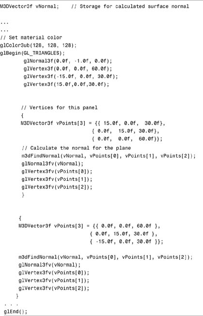
Notice that we are calculating the normal vector using the m3dFindNormal function from math3d. Also, the material properties are now following the colors set by glColor. One other thing you notice is that not every triangle is blocked by glBegin/glEnd functions. You can specify once that you are drawing triangles, and every three vertices are used for a new triangle until you specify otherwise with glEnd. For very large numbers of polygons, this technique can considerably boost performance by eliminating many unnecessary function calls and primitive batch setup.
Figure 5.27 shows the output from the completed LITJET sample program. The jet is now a single shade of gray instead of multiple colors. We changed the color to make it easier to see the lighting effects on the surface. Even though the plane is one solid “color,” you can still see the shape due to the lighting. By rotating the jet around with the arrow keys, you can see the dramatic shading effects as the surface of the jet moves and interacts with the light.
Figure 5.27. The output from the LITJET program.

Lighting Effects
The ambient and diffuse lights from the LITJET example are sufficient to provide the illusion of lighting. The surface of the jet appears shaded according to the angle of the incident light. As the jet rotates, these angles change and you can see the lighting effects changing in such a way that you can easily guess where the light is coming from.
We ignored the specular component of the light source, however, as well as the specular reflectivity of the material properties on the jet. Although the lighting effects are pronounced, the surface of the jet is rather flatly colored. Ambient and diffuse lighting and material properties are all you need if you are modeling clay, wood, cardboard, cloth, or some other flatly colored object. But for metallic surfaces such as the skin of an airplane, some shine is often desirable.
Specular Highlights
Specular lighting and material properties add needed gloss to the surface of your objects. This shininess has a brightening effect on an object’s color and can produce specular highlights when the angle of incident light is sharp in relation to the viewer. A specular highlight is what occurs when nearly all the light striking the surface of an object is reflected away. The white sparkle on a shiny red ball in the sunlight is a good example of a specular highlight.
Specular Light
You can easily add a specular component to a light source. The following code shows the light source setup for the LITJET program, modified to add a specular component to the light:
// Light values and coordinates
GLfloat ambientLight[] = { 0.3f, 0.3f, 0.3f, 1.0f };
GLfloat diffuseLight[] = { 0.7f, 0.7f, 0.7f, 1.0f };
GLfloat specular[] = { 1.0f, 1.0f, 1.0f, 1.0f};
...
...
// Enable lighting
glEnable(GL_LIGHTING);
// Set up and enable light 0
glLightfv(GL_LIGHT0,GL_AMBIENT,ambientLight);
glLightfv(GL_LIGHT0,GL_DIFFUSE,diffuseLight);
glLightfv(GL_LIGHT0,GL_SPECULAR,specular);
glEnable(GL_LIGHT0);
The specular[] array specifies a very bright white light source for the specular component of the light. Our purpose here is to model bright sunlight. The following line simply adds this specular component to the light source GL_LIGHT0:
glLightfv(GL_LIGHT0,GL_SPECULAR,specular);
If this were the only change you made to LITJET, you wouldn’t see any difference in the jet’s appearance. We haven’t yet defined any specular reflectance properties for the material properties.
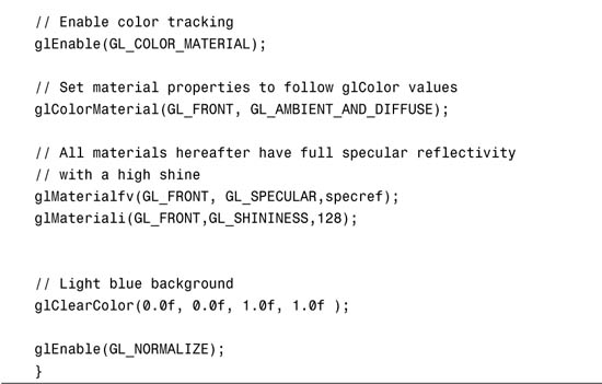
Specular Reflectance
Adding specular reflectance to material properties is just as easy as adding the specular component to the light source. This next code segment shows the code from LITJET, again modified to add specular reflectance to the material properties:
// Light values and coordinates
GLfloat specref[] = { 1.0f, 1.0f, 1.0f, 1.0f };
...
...
// Enable color tracking
glEnable(GL_COLOR_MATERIAL);
// Set material properties to follow glColor values
glColorMaterial(GL_FRONT, GL_AMBIENT_AND_DIFFUSE);
// All materials hereafter have full specular reflectivity
// with a high shine
glMaterialfv(GL_FRONT, GL_SPECULAR,specref);
glMateriali(GL_FRONT,GL_SHININESS,128);
As before, we enable color tracking so that the ambient and diffuse reflectance of the materials follows the current color set by the glColor functions. (Of course, we don’t want the specular reflectance to track glColor because we are specifying it separately and it doesn’t change.)
Now, we’ve added the array specref[], which contains the RGBA values for our specular reflectance. This array of all 1s produces a surface that reflects nearly all incident specular light. The following line sets the material properties for all subsequent polygons to have this reflectance:
glMaterialfv(GL_FRONT, GL_SPECULAR,specref);
Because we do not call glMaterial again with the GL_SPECULAR property, all materials have this property. We set up the example this way on purpose because we want the entire jet to appear made of metal or very shiny composites.
What we have done here in our setup routine is important: We have specified that the ambient and diffuse reflective material properties of all future polygons (until we say otherwise with another call to glMaterial or glColorMaterial) change as the current color changes, but that the specular reflective properties remain the same.
Specular Exponent
As stated earlier, high specular light and reflectivity brighten the colors of the object. For this example, the present extremely high specular light (full intensity) and specular reflectivity (full reflectivity) result in a jet that appears almost totally white or gray except where the surface points away from the light source (in which case, it is black and unlit). To temper this effect, we use the next line of code after the specular component is specified:
glMateriali(GL_FRONT,GL_SHININESS,128);
The GL_SHININESS property sets the specular exponent of the material, which specifies how small and focused the specular highlight is. A value of 0 specifies an unfocused specular highlight, which is actually what is producing the brightening of the colors evenly across the entire polygon. If you set this value, you reduce the size and increase the focus of the specular highlight, causing a shiny spot to appear. The larger the value, the more shiny and pronounced the surface. The range of this parameter is 1–128 for all conformant implementations of OpenGL.
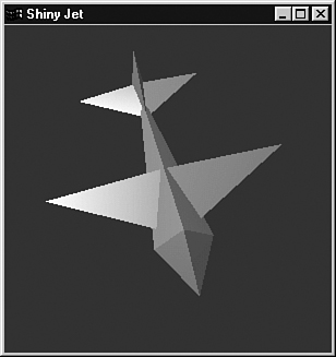
Listing 5.5 shows the new SetupRC code in the sample program SHINYJET. This is the only code that has changed from LITJET (other than the title of the window) to produce a very shiny and glistening jet. Figure 5.28 shows the output from this program, but to fully appreciate the effect, you should run the program and hold down one of the arrow keys to spin the jet about in the sunlight.
Figure 5.28. The output from the SHINYJET program.
Listing 5.5. Setup from SHINYJET to Produce Specular Highlights on the Jet

Normal Averaging
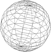
Earlier, we mentioned that by “tweaking” your normals, you can produce apparently smooth surfaces with flat polygons. This technique, known as normal averaging, produces some interesting optical illusions. Say you have a sphere made up of quads and triangles like the one shown in Figure 5.29.
Figure 5.29. A typical sphere made up of quads and triangles.
If each face of the sphere had a single normal specified, the sphere would look like a large faceted jewel. If you specify the “true” normal for each vertex, however, the lighting calculations at each vertex produce values that OpenGL smoothly interpolates across the face of the polygon. Thus, the flat polygons are shaded as if they were a smooth surface.
What do we mean by “true” normal? The polygonal representation is only an approximation of the true surface. Theoretically, if we used enough polygons, the surface would appear smooth. This is similar to the idea we used in Chapter 3, “Drawing in Space: Geometric Primitives and Buffers,” to draw a smooth curve with a series of short line segments. If we consider each vertex to be a point on the true surface, the actual normal value for that surface is the true normal for the surface.
For our case of the sphere, the normal would point directly out from the center of the sphere through each vertex. We show this graphically for a simple 2D case in Figures 5.30 and 5.31. In Figure 5.30, each flat segment has a normal pointing perpendicular to its surface. We did this just like we did for our LITJET example previously. Figure 5.31, however, shows how each normal is not perpendicular to the line segment but is perpendicular to the surface of the sphere, or the tangent line to the surface.
Figure 5.30. An approximation with normals perpendicular to each face.

Figure 5.31. Each normal is perpendicular to the surface itself.
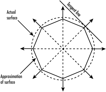
The tangent line touches the curve in one place and does not penetrate it. The 3D equivalent is a tangent plane. In Figure 5.31, you can see the outline of the actual surface and that the normal is actually perpendicular to the line tangent to the surface.
For a sphere, calculation of the normal is reasonably simple. (The normal actually has the same values as the vertex relative to the center!) For other nontrivial surfaces, the calculation might not be so easy. In such cases, you calculate the normals for each polygon that shares a vertex. The actual normal you assign to that vertex is the average of these normals. The visual effect is a nice, smooth, regular surface, even though it is actually composed of numerous small, flat segments.
Putting It All Together
Now it’s time for a more complex sample program. We demonstrate how to use normals to create a smooth surface appearance, move a light around in a scene, create a spotlight, and, finally, identify one of the drawbacks of OpenGL vertex-based lighting.
Our next sample program, SPOT, performs all these tasks. Here, we create a solid sphere in the center of our viewing volume with glutSolidSphere. We shine a spotlight on this sphere that we can move around, and we change the “smoothness” of the normals and demonstrate some of the limitations of OpenGL lighting.
So far, we have been specifying a light’s position with glLight as follows:
// Array to specify position
GLfloat lightPos[] = { 0.0f, 150.0f, 150.0f, 1.0f };
...
...
// Set the light position
glLightfv(GL_LIGHT0,GL_POSITION,lightPos);
The array lightPos[] contains the x, y, and z values that specify either the light’s actual position in the scene or the direction from which the light is coming. The last value, 1.0 in this case, indicates that the light is actually present at this location. By default, the light radiates equally in all directions from this location, but you can change this default to make a spotlight effect.
To make a light source an infinite distance away and coming from the direction specified by this vector, you place 0.0 in this last lightPos[] array element. A directional light source, as this is called, strikes the surface of your objects evenly. That is, all the light rays are parallel. In a positional light source, on the other hand, the light rays diverge from the light source.
Creating a Spotlight
Creating a spotlight is no different from creating any other positional light source. The code in Listing 5.6 shows the SetupRC function from the SPOT sample program. This program places a blue sphere in the center of the window. It also creates a spotlight that you can move vertically with the up- and down-arrow keys and horizontally with the left- and right-arrow keys. As the spotlight moves over the surface of the sphere, a specular highlight follows it on the surface.
Listing 5.6. Lighting Setup for the SPOT Sample Program

The following line from the listing is actually what makes a positional light source into a spotlight:
// Specific spot effects
// Cut-off angle is 60 degrees
glLightf(GL_LIGHT0,GL_SPOT_CUTOFF,60.0f);
The GL_SPOT_CUTOFF value specifies the radial angle of the cone of light emanating from the spotlight, from the center line to the edge of the cone. For a normal positional light, this value is 180° so that the light is not confined to a cone. In fact, for spotlights, only values from 0° to 90° are valid. Spotlights emit a cone of light, and objects outside this cone are not illuminated. Figure 5.32 shows how this angle translates to the cone width.
Figure 5.32. The angle of the spotlight cone.

Drawing a Spotlight
When you place a spotlight in a scene, the light must come from somewhere. Just because you have a source of light at some location doesn’t mean that you see a bright spot there. For our SPOT sample program, we placed a red cone at the spotlight source to show where the light was coming from. Inside the end of this cone, we placed a bright yellow sphere to simulate a light bulb.
This sample has a pop-up menu that we use to demonstrate several things. The pop-up menu contains items to set flat and smooth shading and to produce a sphere for low, medium, and high approximation. Surface approximation means to break the mesh of a curved surface into a finer mesh of polygons (more vertices). Figure 5.33 shows a wireframe representation of a highly approximated sphere next to one that has few polygons.
Figure 5.33. On the left is a highly approximated sphere; on the right, a sphere made up of fewer polygons.

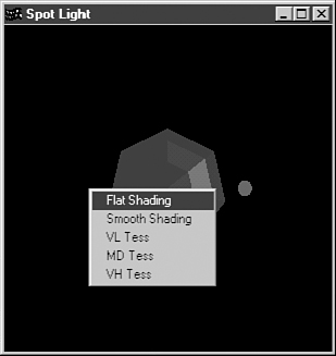
Figure 5.34 shows our sample in its initial state with the spotlight moved off slightly to one side. (You can use the arrow keys to move the spotlight.) The sphere consists of a few polygons, which are flat shaded. In Windows, use the right mouse button to open a pop-up menu (Ctrl-click on the Mac) where you can switch between smooth and flat shading and between very low, medium, and very high approximation for the sphere. Listing 5.7 shows the complete code for rendering the scene.
Figure 5.34. The SPOT sample—low approximation, flat shading.
Listing 5.7. The Rendering Function for SPOT, Showing How the Spotlight Is Moved


The variables iTess and iMode are set by the GLUT menu handler and control how many sections the sphere is broken into and whether flat or smooth shading is employed. Note that the light is positioned before any geometry is rendered. As pointed out in Chapter 2, OpenGL is an immediate-mode API: If you want an object to be illuminated, you have to put the light where you want it before drawing the object.
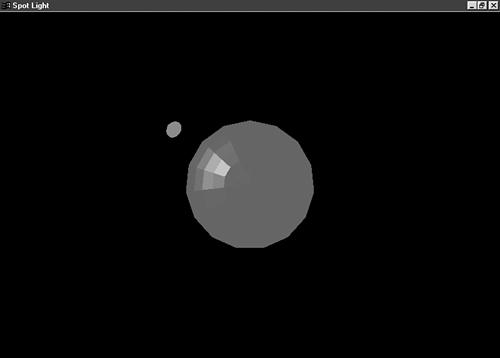
You can see in Figure 5.34 that the sphere is coarsely lit and each flat face is clearly evident. Switching to smooth shading helps a little, as shown in Figure 5.35.
Figure 5.35. Smoothly shaded but inadequate approximation.
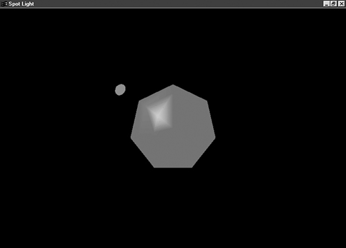
Increasing the approximation helps, as shown in Figure 5.36, but you still see disturbing artifacts as you move the spotlight around the sphere. These lighting artifacts are one of the drawbacks of OpenGL lighting. A better way to characterize this situation is to say that these artifacts are a drawback of vertex lighting (not necessarily OpenGL!). By lighting the vertices and then interpolating between them, we get a crude approximation of lighting. This approach is sufficient for many cases, but as you can see in our spot example, it is not sufficient in others. If you switch to very high approximation and move the spotlight, you see the lighting blemishes all but vanish.
Figure 5.36. Choosing a finer mesh of polygons yields better vertex lighting.

With most OpenGL hardware implementations accelerating transformations and lighting effects, we are able to more finely approximate geometry for better OpenGL-based lighting effects. For the very best quality light effects, we will turn to shaders, in Part III, “The Apocrypha.”
The final observation you need to make about the SPOT sample appears when you set the sphere for medium approximation and flat shading. As shown in Figure 5.37, each face of the sphere is flatly lit. Each vertex is the same color but is modulated by the value of the normal and the light. With flat shading, each polygon is made the color of the last vertex color specified and not smoothly interpolated between each one.
Figure 5.37. A multifaceted sphere.
Shadows
A chapter on color and lighting naturally calls for a discussion of shadows. Adding shadows to your scenes can greatly improve their realism and visual effectiveness. In Figures 5.38 and 5.39, you see two views of a lighted cube. Although both are lit, the one with a shadow is more convincing than the one without the shadow.
Figure 5.38. A lighted cube without a shadow.

Figure 5.39. A lighted cube with a shadow.

What Is a Shadow?
Conceptually, drawing a shadow is quite simple. A shadow is produced when an object keeps light from a light source from striking some object or surface behind the object casting the shadow. The area on the shadowed object’s surface, outlined by the object casting the shadow, appears dark. We can produce a shadow programmatically by flattening the original object into the plane of the surface in which the object lies. The object is then drawn in black or some dark color, perhaps with some translucence. There are many methods and algorithms for drawing shadows, some quite complex. This book’s primary focus is on the OpenGL API. It is our hope that, after you’ve mastered the tool, some of the additional reading suggested in Appendix A will provide you with a lifetime of learning new applications for this tool. Chapter 14, “Depth Textures and Shadows,” covers some new direct support in OpenGL for making shadows; for our purposes in this chapter, we demonstrate one of the simpler methods that works quite well when casting shadows on a flat surface (such as the ground). Figure 5.40 illustrates this flattening.
Figure 5.40. Flattening an object to create a shadow.

We squish an object against another surface by using some of the advanced matrix manipulations we touched on in the preceding chapter. Here, we boil down this process to make it as simple as possible.
Squish Code
We need to flatten the modelview projection matrix so that any and all objects drawn into it are now in this flattened two-dimensional world. No matter how the object is oriented, it is projected (squished) into the plane in which the shadow lies. The next two considerations are the distance and direction of the light source. The direction of the light source determines the shape of the shadow and influences the size. If you’ve ever seen your shadow in the early or late hours, you know how long and warped your shadow can appear, depending on the position of the sun.
The function m3dMakePlanarShadowMatrix from the math3d library, shown in Listing 5.8, takes the plane equation of the plane in which you want the shadow to appear (three points that cannot be along the same straight line can be fed to m3dGetPlaneEquation to get the equation of the plane), and the position of the light source, and returns a transformation matrix that this function constructs. Without delving into the linear algebra, what this function does is build a transformation matrix. If you multiply this matrix by the current modelview matrix, all further drawing is flattened into this plane.
A Shadow Example
To demonstrate the use of this shadow matrix, we suspend our jet in air high above the ground. We place the light source directly above and a bit to the left of the jet. As you use the arrow keys to spin the jet around, the shadow cast by the jet appears flattened on the ground below. The output from this SHADOW sample program is shown in Figure 5.41.
Figure 5.41. The output from the SHADOW sample program.

The code in Listing 5.8 shows how the shadow projection matrix was created for this example. Note that we create the matrix once in SetupRC and save it in a global variable.
Listing 5.8. Setting Up the Shadow Projection Matrix

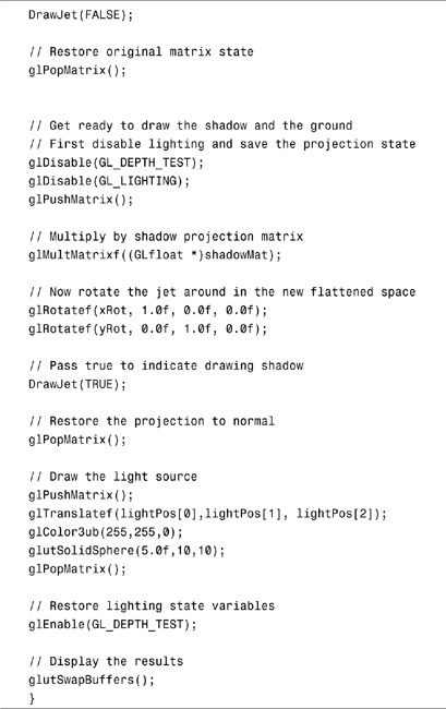
Listing 5.9 shows the rendering code for the shadow example. We first draw the ground. Then we draw the jet as we normally do, restore the modelview matrix, and multiply it by the shadow matrix. This procedure creates our squish matrix. Then we draw the jet again. (We’ve modified our code to accept a flag telling the DrawJet function to render in color or black.) After restoring the modelview matrix once again, we draw a small yellow sphere to approximate the position of the light. Note that we disable depth testing before we draw a plane below the jet to indicate the ground.
This rectangle lies in the same plane in which our shadow is drawn, and we want to make sure the shadow is drawn. We have never before discussed what happens if we draw two objects or planes in the same location. We have discussed depth testing as a means to determine what is drawn in front of what, however. If two objects occupy the same location, usually the last one drawn is shown. Sometimes, however, an effect called z-fighting causes fragments from both objects to be intermingled, resulting in a mess!
Listing 5.9. Rendering the Jet and Its Shadow

Sphere World Revisited
Our last example for this chapter is too long to list the source code in its entirety. In the preceding chapter’s SPHEREWORLD sample program, we created an immersive 3D world with animation and camera movement. In this chapter, we’ve revisited Sphere World and have added lights and material properties to the torus and sphere inhabitants. Finally, we have also used our planar shadow technique to add a shadow to the ground! We will keep coming back to this example from time to time as we add more and more of our OpenGL functionality to the code. The output of this chapter’s version of SPHEREWORLD is shown in Figure 5.42.
Figure 5.42. Fully lit and shadowed Sphere World.

Summary
This chapter introduced some of the more magical and powerful capabilities of OpenGL. We started by adding color to 3D scenes, as well as smooth shading. We then saw how to specify one or more light sources and define their lighting characteristics in terms of ambient, diffuse, and specular components. We explained how the corresponding material properties interact with these light sources and demonstrated some special effects, such as adding specular highlights and softening sharp edges between adjoining triangles.
Also covered were lighting positions and the creation and manipulation of spotlights. The high-level matrix munching function presented here makes shadow generation as easy as it gets for planar shadows.