
Chapter 10. Curves and Surfaces
WHAT YOU’LL LEARN IN THIS CHAPTER:

The practice of 3D graphics is little more than a computerized version of connect-the-dots. Vertices are laid out in 3D space and connected by flat primitives. Smooth curves and surfaces are approximated using flat polygons and shading tricks. The more polygons used, usually the more smooth and curved a surface may appear. OpenGL, of course, supports smooth curves and surfaces implicitly because you can specify as many vertices as you want and set any desired or calculated values for normals and color values.
OpenGL does provide some additional support, however, that makes the task of constructing more complex surfaces a bit easier. The easiest to use are some GLU functions that render spheres, cylinders, cones (special types of cylinders, as you will see), and flat, round disks, optionally with holes in them. OpenGL also provides top-notch support for complex surfaces that may be difficult to model with a simple mathematical equation: Bézier and NURB curves and surfaces. Finally, OpenGL can take large, irregular, and concave polygons and break them up into smaller, more manageable pieces.
Built-in Surfaces
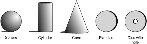
The OpenGL Utility Library (GLU) that accompanies OpenGL contains a number of functions that render three quadratic surfaces. These quadric functions render spheres, cylinders, and disks. You can specify the radius of both ends of a cylinder. Setting one end’s radius to 0 produces a cone. Disks, likewise, provide enough flexibility for you to specify a hole in the center (producing a washer-like surface). You can see these basic shapes illustrated graphically in Figure 10.1.
Figure 10.1. Possible quadric shapes.
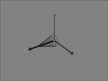
These quadric objects can be arranged to create more complex models. For example, you could create a 3D molecular modeling program using just spheres and cylinders. Figure 10.2 shows the 3D unit axes drawn with a sphere, three cylinders, three cones, and three disks. This model can be included in any of your own programs via the following glTools function:
void gltDrawUnitAxes(void)
Figure 10.2. The x,y,z-axes drawn with quadrics.

Setting Quadric States
The quadric surfaces can be drawn with some flexibility as to whether normals, texture coordinates, and so on are specified. Putting all these options into parameters to a sphere drawing function, for example, would create a function with an exceedingly long list of parameters that must be specified each time. Instead, the quadric functions use an object-oriented model. Essentially, you create a quadric object and set its rendering state with one or more state setting functions. Then you specify this object when drawing one of the surfaces, and its state determines how the surface is rendered. The following code segment shows how to create an empty quadric object and later delete it:
GLUquadricObj *pObj;
// . . .
pObj = gluNewQuadric(); // Create and initialize Quadric
// Set Quadric rendering Parameters
// Draw Quadric surfaces
// . . .
gluDeleteQuadric(pObj); // Free Quadric object
Note that you create a pointer to the GLUQuadricObj data type, not an instance of the data structure itself. The reason is that the gluNewQuadric function not only allocates space for it, but also initializes the structure members to reasonable default values. Do not confuse these quadric objects with C++ classes; they are really just C data structures.
There are four functions you can use to modify the drawing state of the GLUQuadricObj object and, correspondingly, to any surfaces drawn with it. The first function sets the quadric draw style:
void gluQuadricDrawStyle(GLUquadricObj *obj, GLenum drawStyle);
The first parameter is the pointer to the quadric object to be set, and the drawStyle parameter is one of the values in Table 10.1.
Table 10.1. Quadric Draw Styles

The next function specifies whether the quadric surface geometry would be generated with surface normals:
void gluQuadricNormals(GLUquadricObj *pbj, GLenum normals);
Quadrics may be drawn without normals (GLU_NONE), with smooth normals (GLU_SMOOTH), or flat normals (GLU_FLAT). The primary difference between smooth and flat normals is that for smooth normals, one normal is specified for each vertex perpendicular to the surface being approximated, giving a smoothed-out appearance. For flat normals, all normals are face normals, perpendicular to the actual triangle (or quad) face.
You can also specify whether the normals point out of the surface or inward. For example, looking at a lit sphere, you would want normals pointing outward from the surface of the sphere. However, if you were drawing the inside of a sphere—say, as part of a vaulted ceiling—you would want the normals and lighting to be applied to the inside of the sphere. The following function sets this parameter:
void gluQuadricOrientation(GLUquadricObj *obj, GLenum orientation);
Here, orientation can be either GLU_OUTSIDE or GLU_INSIDE. By default, quadric surfaces are wound counterclockwise, with the front faces facing the outsides of the surfaces. The outside of the surface is intuitive for spheres and cylinders; for disks, it is simply the side facing the positive z-axis.
Finally, you can request that texture coordinates be generated for quadric surfaces with the following function:
void gluQuadricTexture(GLUquadricObj *obj, GLenum textureCoords);
Here, the textureCoords parameter can be either GL_TRUE or GL_FALSE. When texture coordinates are generated for quadric surfaces, they are wrapped around spheres and cylinders evenly; they are applied to disks using the center of the texture for the center of the disk, with the edges of the texture lining up with the edges of the disk.
Drawing Quadrics
After the quadric object state has been set satisfactorily, each surface is drawn with a single function call. For example, to draw a sphere, you simply call the following function:
void gluSphere(GLUQuadricObj *obj, GLdouble radius, GLint slices, GLint stacks);
The first parameter, obj, is just the pointer to the quadric object that was previously set up for the desired rendering state. The radius parameter is then the radius of the sphere, followed by the number of slices and stacks. Spheres are drawn with rings of triangle strips (or quad strips, depending on whose GLU library you’re using) stacked from the bottom to the top, as shown in Figure 10.3. The number of slices specifies how many triangle sets (or quads) are used to go all the way around the sphere. You could also think of this as the number of lines of latitude and longitude around a globe.
Figure 10.3. A quadric sphere’s stacks and slices.

The quadric spheres are drawn on their sides with the positive z-axis pointing out the top of the spheres. Figure 10.4 shows a wireframe quadric sphere drawn around the unit axes.
Figure 10.4. A quadric sphere’s orientation.

Cylinders are also drawn along the positive z-axis and are composed of a number of stacked strips. The following function, which is similar to the gluSphere function, draws a cylinder:
void gluCylinder(GLUquadricObj *obj, GLdouble baseRadius,
GLdouble topRadius, GLdouble height,
GLint slices, GLint stacks);
With this function, you can specify both the base radius (near the origin) and the top radius (out along the positive z-axis). The height parameter is simply the length of the cylinder. The orientation of the cylinder is shown in Figure 10.5. Figure 10.6 shows the same cylinder, but with the topRadius parameter set to 0, making a cone.
Figure 10.5. A quadric cylinder’s orientation.

Figure 10.6. A quadric cone made from a cylinder.
The final quadric surface is the disk. Disks are drawn with loops of quads or triangle strips, divided into some number of slices. You use the following function to render a disk:
void gluDisk(GLUquadricObj *obj, GLdouble innerRadius,
GLdouble outerRadius, GLint slices, GLint loops);
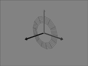
To draw a disk, you specify both an inner radius and an outer radius. If the inner radius is 0, you get a solid disk like the one shown in Figure 10.7. A nonzero radius gives you a disk with a hole in it, as shown in Figure 10.8. The disk is drawn in the xy plane.
Figure 10.7. A quadric disk showing loops and slices.

Figure 10.8. A quadric disk with a hole in the center.
Modeling with Quadrics
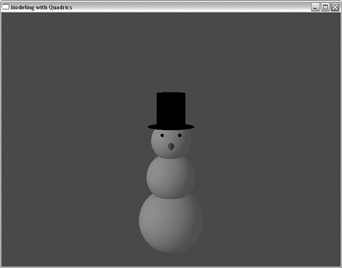
In the sample program SNOWMAN, all the quadric objects are used to piece together a crude model of a snowman. White spheres make up the three sections of the body. Two small black spheres make up the eyes, and an orange cone is drawn for the carrot nose. A cylinder is used for the body of a black top hat, and two disks, one closed and one open, provide the top and the rim of the hat. The output from SNOWMAN is shown in Figure 10.9. Listing 10.1 shows the rendering code that draws the snowman by simply transforming the various quadric surfaces into their respective positions.
Figure 10.9. A snowman rendered from quadric objects.
Listing 10.1. Rendering Code for the SNOWMAN Example


Bézier Curves and Surfaces
Quadrics provide built-in support for some very simple surfaces easily modeled with algebraic equations. Suppose, however, you want to create a curve or surface, and you don’t have an algebraic equation to start with. It’s far from a trivial task to figure out your surface in reverse, starting from what you visualize as the result and working down to a second- or third-order polynomial. Taking a rigorous mathematical approach is time consuming and error-prone, even with the aid of a computer. You can also forget about trying to do it in your head.
Recognizing this fundamental need in the art of computer-generated graphics, Pierre Bézier, an automobile designer for Renault in the 1970s, created a set of mathematical models that could represent curves and surfaces by specifying only a small set of control points. In addition to simplifying the representation of curved surfaces, the models facilitated interactive adjustments to the shape of the curve or surface.
Other types of curves and surfaces and indeed a whole new vocabulary for computer-generated surfaces soon evolved. The mathematics behind this magic show are no more complex than the matrix manipulations in Chapter 4, “Geometric Transformations: The Pipeline,” and an intuitive understanding of these curves is easy to grasp. As we did in Chapter 4, we take the approach that you can do a lot with these functions without a deep understanding of their mathematics.
Parametric Representation
A curve has a single starting point, a length, and an endpoint. It’s really just a line that squiggles about in 3D space. A surface, on the other hand, has width and length and thus a surface area. We begin by showing you how to draw some smooth curves in 3D space and then extend this concept to surfaces. First, let’s establish some common vocabulary and math fundamentals.
When you think of straight lines, you might think of this famous equation:
y = mx + b
Here, m equals the slope of the line, and b is the y intercept of the line (the place where the line crosses the y-axis). This discussion might take you back to your eighth-grade algebra class, where you also learned about the equations for parabolas, hyperbolas, exponential curves, and so on. All these equations expressed y (or x) in terms of some function of x (or y).
Another way of expressing the equation for a curve or line is as a parametric equation. A parametric equation expresses both x and y in terms of another variable that varies across some predefined range of values that is not explicitly a part of the geometry of the curve. Sometimes in physics, for example, the x, y, and z coordinates of a particle might be in terms of some functions of time, where time is expressed in seconds. In the following, f(), g(), and h() are unique functions that vary with time (t):
x = f(t)
y = g(t)
z = h(t)
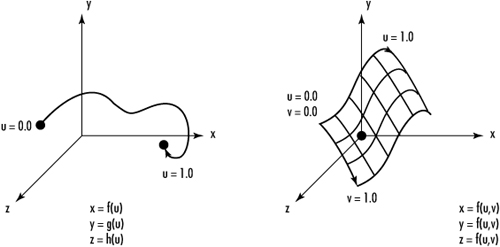
When we define a curve in OpenGL, we also define it as a parametric equation. The parametric parameter of the curve, which we call u, and its range of values is the domain of that curve. Surfaces are described using two parametric parameters: u and v. Figure 10.10 shows both a curve and a surface defined in terms of u and v domains. The important point to realize here is that the parametric parameters (u and v) represent the extents of the equations that describe the curve; they do not reflect actual coordinate values.
Figure 10.10. Parametric representation of curves and surfaces.
Control Points
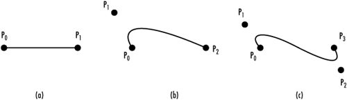
A curve is represented by a number of control points that influence the shape of the curve. For a Bézier curve, the first and last control points are actually part of the curve. The other control points act as magnets, pulling the curve toward them. Figure 10.11 shows some examples of this concept, with varying numbers of control points.
Figure 10.11. How control points affect curve shape.
The order of the curve is represented by the number of control points used to describe its shape. The degree is one less than the order of the curve. The mathematical meaning of these terms pertains to the parametric equations that exactly describe the curve, with the order being the number of coefficients and the degree being the highest exponent of the parametric parameter. If you want to read more about the mathematical basis of Bézier curves, see Appendix A, “Further Reading/References.”
The curve in Figure 10.11(b) is called a quadratic curve (degree 2), and Figure 10.11(c) is called a cubic (degree 3). Cubic curves are the most typical. Theoretically, you could define a curve of any order, but higher order curves start to oscillate uncontrollably and can vary wildly with the slightest change to the control points.
Continuity
If two curves placed side by side share an endpoint (called the breakpoint), they together form a piecewise curve. The continuity of these curves at this breakpoint describes how smooth the transition is between them. The four categories of continuity are none, positional (C0), tangential (C1), and curvature (C2).
As you can see in Figure 10.12, no continuity occurs when the two curves don’t meet at all. Positional continuity is achieved when the curves at least meet and share a common endpoint. Tangential continuity occurs when the two curves have the same tangent at the breakpoint. Finally, curvature continuity means the two curves’ tangents also have the same rate of change at the breakpoint (thus an even smoother transition).
Figure 10.12. Continuity of piecewise curves.

When assembling complex surfaces or curves from many pieces, you usually strive for tangential or curvature continuity. You’ll see later that some parameters for curve and surface generation can be chosen to produce the desired continuity.
Evaluators
OpenGL contains several functions that make it easy to draw Bézier curves and surfaces. To draw them, you specify the control points and the range for the parametric u and v parameters. Then, by calling the appropriate evaluation function (the evaluator), OpenGL generates the points that make up the curve or surface. We start with a 2D example of a Bézier curve and then extend it to three dimensions to create a Bézier surface.
A 2D Curve
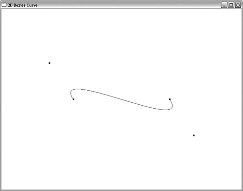
The best way to start is to go through an example, explaining it line by line. Listing 10.2 shows some code from the sample program BEZIER in this chapter’s subdirectory of the source code distribution on our Web site. This program specifies four control points for a Bézier curve and then renders the curve using an evaluator. The output from Listing 10.2 is shown in Figure 10.13.
Listing 10.2. Code from BEZIER That Draws a Bézier Curve with Four Control Points

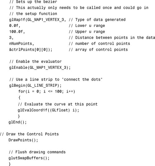

Figure 10.13. Output from the BEZIER sample program.
The first thing we do in Listing 10.2 is define the control points for our curve:
// The number of control points for this curve
GLint nNumPoints = 4;
GLfloat ctrlPoints[4][3]= {{ -4.0f, 0.0f, 0.0f}, // Endpoint
{ -6.0f, 4.0f, 0.0f}, // Control point
{ 6.0f, -4.0f, 0.0f}, // Control point
{ 4.0f, 0.0f, 0.0f }}; // Endpoint
We defined global variables for the number of control points and the array of control points. To experiment, you can change them by adding more control points or just modifying the position of these points.
The DrawPoints function is reasonably straightforward. We call this function from our rendering code to display the control points along with the curve. This capability also is useful when you’re experimenting with control-point placement. Our standard ChangeSize function establishes a 2D orthographic projection that spans from –10 to +10 in the x and y directions.
Finally, we get to the rendering code. The RenderScene function first calls glMap1f (after clearing the screen) to create a mapping for our curve:
// Called to draw scene
void RenderScene(void)
{
int i;
// Clear the window with current clearing color
glClear(GL_COLOR_BUFFER_BIT);
// Sets up the Bezier
// This actually only needs to be called once and could go in
// the setup function
glMap1f(GL_MAP1_VERTEX_3, // Type of data generated
0.0f, // Lower u range
100.0f, // Upper u range
3, // Distance between points in the data
nNumPoints, // Number of control points
&ctrlPoints[0][0]); // Array of control points
...
...
The first parameter to glMap1f, GL_MAP1_VERTEX_3, sets up the evaluator to generate vertex coordinate triplets (x, y, and z). You can also have the evaluator generate other values, such as texture coordinates and color information. See Appendix C, “API Reference,” for details.
The next two parameters specify the lower and upper bounds of the parametric u value for this curve. The lower value specifies the first point on the curve, and the upper value specifies the last point on the curve. All the values in between correspond to the other points along the curve. Here, we set the range to 0–100.
The fourth parameter to glMap1f specifies the number of floating-point values between the vertices in the array of control points. Each vertex consists of three floating-point values (for x, y, and z), so we set this value to 3. This flexibility allows the control points to be placed in an arbitrary data structure, as long as they occur at regular intervals.
The last parameter is a pointer to a buffer containing the control points used to define the curve. Here, we pass a pointer to the first element of the array. After creating the mapping for the curve, we enable the evaluator to make use of this mapping. This capability is maintained through a state variable, and the following function call is all that is needed to enable the evaluator to produce points along the curve:
// Enable the evaluator
glEnable(GL_MAP1_VERTEX_3);
The glEvalCoord1f function takes a single argument: a parametric value along the curve. This function then evaluates the curve at this value and calls glVertex internally for that point. By looping through the domain of the curve and calling glEvalCoord to produce vertices, we can draw the curve with a simple line strip:
// Use a line strip to "connect the dots"
glBegin(GL_LINE_STRIP);
for(i = 0; i <= 100; i++)
{
// Evaluate the curve at this point
glEvalCoord1f((GLfloat) i);
}
glEnd();
Finally, we want to display the control points themselves:
// Draw the control points
DrawPoints();
Evaluating a Curve
OpenGL can make things even easier than what we’ve done so far. We set up a grid with the glMapGrid function, which tells OpenGL to create an evenly spaced grid of points over the u domain (the parametric argument of the curve). Then we call glEvalMesh to “connect the dots” using the primitive specified (GL_LINE or GL_POINTS). The two function calls
// Use higher level functions to map to a grid, then evaluate the
// entire thing.
// Map a grid of 100 points from 0 to 100
glMapGrid1d(100,0.0,100.0);
// Evaluate the grid, using lines
glEvalMesh1(GL_LINE,0,100);
completely replace this code:
// Use a line strip to "connect the dots"
glBegin(GL_LINE_STRIP);
for(i = 0; i <= 100; i++)
{
// Evaluate the curve at this point
glEvalCoord1f((GLfloat) i);
}
glEnd();
As you can see, this approach is more compact and efficient, but its real benefit comes when evaluating surfaces rather than curves.
A 3D Surface
Creating a 3D Bézier surface is much like creating the 2D version. In addition to defining points along the u domain, we must define them along the v domain. Listing 10.3 contains code from our next sample program, BEZ3D, and displays a wire mesh of a 3D Bézier surface. The first change from the preceding example is that we have defined three more sets of control points for the surface along the v domain. To keep this surface simple, we’ve kept the same control points except for the z value. This way, we create a uniform surface, as if we simply extruded a 2D Bézier along the z-axis.
Listing 10.3. BEZ3D Code to Create a Bézier Surface

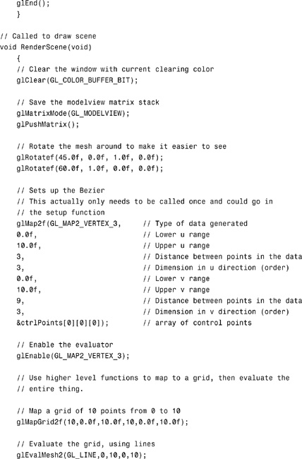
Our rendering code is different now, too. In addition to rotating the figure for a better visual effect, we call glMap2f instead of glMap1f. This call specifies control points along two domains (u and v) instead of just one (u):
// Sets up the Bezier
// This actually only needs to be called once and could go in
// the setup function
glMap2f(GL_MAP2_VERTEX_3, // Type of data generated
0.0f, // Lower u range
10.0f, // Upper u range
3, // Distance between points in the data
3, // Dimension in u direction (order)
0.0f, // Lower v range
10.0f, // Upper v range
9, // Distance between points in the data
3, // Dimension in v direction (order)
&ctrlPoints[0][0][0]); // Array of control points
We must still specify the lower and upper range for u, and the distance between points in the u domain is still three. Now, however, we must also specify the lower and upper range in the v domain. The distance between points in the v domain is now nine values because we have a three-dimensional array of control points, with each span in the u domain being three points of three values each (3 × 3 = 9). Then we tell glMap2f how many points in the v direction are specified for each u division, followed by a pointer to the control points themselves.
The two-dimensional evaluator is enabled just like the one-dimensional version, and we call glMapGrid2f with the number of divisions in the u and v direction:
// Enable the evaluator
glEnable(GL_MAP2_VERTEX_3);
// Use higher level functions to map to a grid, then evaluate the
// entire thing.
// Map a grid of 10 points from 0 to 10
glMapGrid2f(10,0.0f,10.0f,10,0.0f,10.0f);
After the evaluator is set up, we can call the two-dimensional (meaning u and v) version of glEvalMesh to evaluate our surface grid. Here, we evaluate using lines and specify the u and v domains’ values to range from 0 to 10:
// Evaluate the grid, using lines
glEvalMesh2(GL_LINE,0,10,0,10);
The result is shown in Figure 10.14.
Figure 10.14. Output from the BEZ3D program.

Lighting and Normal Vectors
Another valuable feature of evaluators is the automatic generation of surface normals. By simply changing this code
// Evaluate the grid, using lines
glEvalMesh2(GL_LINE,0,10,0,10);
// Evaluate the grid, using polygons
glEvalMesh2(GL_FILL,0,10,0,10);
and then calling
glEnable(GL_AUTO_NORMAL);
in our initialization code, we enable easy lighting of surfaces generated by evaluators. Figure 10.15 shows the same surface as Figure 10.14, but with lighting enabled and automatic normalization turned on. The code for this program appears in the BEZLIT sample in the subdirectory for this chapter in the source code distribution on our Web site. The program is only slightly modified from BEZ3D.
Figure 10.15. Output from the BEZLIT program.

NURBS
You can use evaluators to your heart’s content to evaluate Bézier surfaces of any degree, but for more complex curves, you have to assemble your Béziers piecewise. As you add more control points, creating a curve that has good continuity becomes difficult. A higher level of control is available through the GLU library’s NURBS functions. NURBS stands for non-uniform rational B-spline. Mathematicians out there might know immediately that this is just a more generalized form of curves and surfaces that can produce Bézier curves and surfaces, as well as some other kinds (mathematically speaking). These functions allow you to tweak the influence of the control points you specified for the evaluators to produce smoother curves and surfaces with larger numbers of control points.
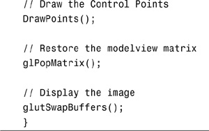
From Bézier to B-Splines
A Bézier curve is defined by two points that act as endpoints and any number of other control points that influence the shape of the curve. The three Bézier curves in Figure 10.16 have three, four, and five control points specified. The curve is tangent to a line that connects the endpoints with their adjacent control points. For quadratic (three points) and cubic (four points) curves, the resulting Béziers are quite smooth, usually with a continuity of C2 (curvature). For higher numbers of control points, however, the smoothness begins to break down as the additional control points pull and tug on the curve.
Figure 10.16. Bézier continuity as the order of the curve increases.
B-splines (bi-cubic splines), on the other hand, work much as the Bézier curves do, but the curve is broken down into segments. The shape of any given segment is influenced only by the nearest four control points, producing a piecewise assemblage of a curve with each segment exhibiting characteristics much like a fourth-order Bézier curve. A long curve with many control points is inherently smoother, with the junction between each segment exhibiting C2 continuity. It also means that the curve does not necessarily have to pass through any of the control points.
Knots
The real power of NURBS is that you can tweak the influence of the four control points for any given segment of a curve to produce the smoothness needed. This control is handled via a sequence of values called knots. Two knot values are defined for every control point. The range of values for the knots matches the u or v parametric domain and must be nondescending. The knot values determine the influence of the control points that fall within that range in u/v space. Figure 10.17 shows a curve demonstrating the influence of control points over a curve having four units in the u parametric domain. Points in the middle of the u domain have a greater pull on the curve, and only points between 0 and 3 have any effect on the shape of the curve.
Figure 10.17. Control-point influence along the u parameter.

The key here is that one of these influence curves exists at each control point along the u/v parametric domain. The knot sequence then defines the strength of the influence of points within this domain. If a knot value is repeated, points near this parametric value have even greater influence. The repeating of knot values is called knot multiplicity. Higher knot multiplicity decreases the curvature of the curve or surface within that region.
Creating a NURBS Surface
The GLU NURBS functions provide a useful high-level facility for rendering surfaces. You don’t have to explicitly call the evaluators or establish the mappings or grids. To render a NURBS, you first create a NURBS object that you reference whenever you call the NURBS related functions to modify the appearance of the surface or curve.
The gluNewNurbsRenderer function creates a renderer for the NURB, and gluDeleteNurbsRenderer destroys it. The following code fragments demonstrate these functions in use:
// NURBS object pointer
GLUnurbsObj *pNurb = NULL;
...
...
// Set up the NURBS object
pNurb = gluNewNurbsRenderer();
...
// Do your NURBS things...
...
...
// Delete the NURBS object if it was created
if(pNurb)
gluDeleteNurbsRenderer(pNurb);
NURBS Properties
After you have created a NURBS renderer, you can set various high-level NURBS properties for the NURB:
// Set sampling tolerance
gluNurbsProperty(pNurb, GLU_SAMPLING_TOLERANCE, 25.0f);
// Fill to make a solid surface (use GLU_OUTLINE_POLYGON to create a
// polygon mesh)
gluNurbsProperty(pNurb, GLU_DISPLAY_MODE, (GLfloat)GLU_FILL);
You typically call these functions in your setup routine rather than repeatedly in your rendering code. In this example, GLU_SAMPLING_TOLERANCE defines the fineness of the mesh that defines the surface, and GLU_FILL tells OpenGL to fill in the mesh instead of generating a wireframe.
Defining the Surface
The surface definition is passed as arrays of control points and knot sequences to the gluNurbsSurface function. As shown here, this function is also bracketed by calls to gluBeginSurface and gluEndSurface:
// Render the NURB
// Begin the NURB definition
gluBeginSurface(pNurb);
// Evaluate the surface
gluNurbsSurface(pNurb, // Pointer to NURBS renderer
8, Knots, // No. of knots and knot array u direction
8, Knots, // No. of knots and knot array v direction
4 * 3, // Distance between control points in u dir.
3, // Distance between control points in v dir.
&ctrlPoints[0][0][0],// Control points
4, 4, // u and v order of surface
GL_MAP2_VERTEX_3); // Type of surface
// Done with surface
gluEndSurface(pNurb);
You can make more calls to gluNurbsSurface to create any number of NURBS surfaces, but the properties you set for the NURBS renderer are still in effect. Often, this is desired; you rarely want two surfaces (perhaps joined) to have different fill styles (one filled and one a wire mesh).
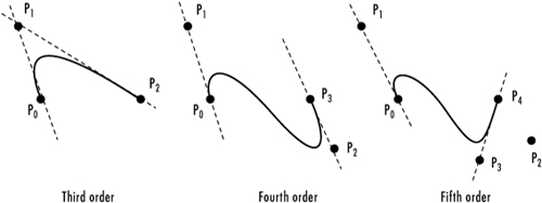
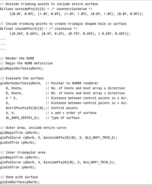
Using the control points and knot values shown in the next code segment, we produced the NURBS surface shown in Figure 10.18. You can find this NURBS program in this chapter’s subdirectory in the source code distribution on our Web site:
Figure 10.18. Output from the NURBS program.

Trimming
Trimming means creating cutout sections from NURBS surfaces. This capability is often used for literally trimming sharp edges of a NURBS surface. You can also create holes in your surface just as easily. The output from the NURBT program is shown in Figure 10.19. This is the same NURBS surface used in the preceding sample (without the control points shown), with a triangular region removed. This program, too, is in the subdirectory for this chapter in the source code distribution on our Web site.
Figure 10.19. Output from the NURBT program.

Listing 10.4 shows the code added to the NURBS sample program to produce this trimming effect. Within the gluBeginSurface/gluEndSurface delimiters, we call gluBeginTrim, specify a trimming curve with gluPwlCurve, and finish the trimming curve with gluEndTrim.
Listing 10.4. Modifications to NURBS to Produce Trimming
Within the gluBeginTrim/gluEndTrim delimiters, you can specify any number of curves as long as they form a closed loop in a piecewise fashion. You can also use gluNurbsCurve to define a trimming region or part of a trimming region. These trimming curves must, however, be in terms of the unit parametric u and v space. This means the entire u/v domain is scaled from 0.0 to 1.0.
gluPwlCurve defines a piecewise linear curve—nothing more than a list of points connected end to end. In this scenario, the inner trimming curve forms a triangle, but with many points, you could create an approximation of any curve needed.
Trimming a curve trims away surface area that is to the right of the curve’s winding. Thus, a clockwise-wound trimming curve discards its interior. Typically, an outer trimming curve is specified, which encloses the entire NURBS parameter space. Then smaller trimming regions are specified within this region with clockwise winding. Figure 10.20 illustrates this relationship.
Figure 10.20. An area inside clockwise-wound curves is trimmed away.

NURBS Curves
Just as you can have Bézier surfaces and curves, you can also have NURBS surfaces and curves. You can even use gluNurbsCurve to do NURBS surface trimming. By this point, we hope you have the basics down well enough to try trimming surfaces on your own. However, another sample, NURBC, is included in the sample source code if you want a starting point to play with.
Tessellation
To keep OpenGL as fast as possible, all geometric primitives must be convex. We made this point in Chapter 3, “Drawing in Space: Geometric Primitives and Buffers.” However, many times we have vertex data for a concave or more complex shape that we want to render with OpenGL. These shapes fall into two basic categories, as shown in Figure 10.21. A simple concave polygon is shown on the left, and a more complex polygon with a hole in it is shown on the right. For the shape on the left, you might be tempted to try using GL_POLYGON as the primitive type, but the rendering would fail because OpenGL algorithms are optimized for convex polygons. As for the figure on the right...well, there is little hope for that shape at all!
Figure 10.21. Some nonconvex polygons.

The intuitive solution to both of these problems is to break down the shape into smaller convex polygons or triangles that can be fit together to create the final overall shape. Figure 10.22 shows one possible solution to breaking the shapes in Figure 10.21 into more manageable triangles.
Figure 10.22. Complex shapes broken down into triangles.

Breaking down the shapes by hand is tedious at best and possibly error-prone. Fortunately, the OpenGL Utility Library contains functions to help you break concave and complex polygons into smaller, valid OpenGL primitives. The process of breaking down these polygons is called tessellation.
The Tessellator
Tessellation works through a tessellator object that must be created and destroyed much in the same way that we did for quadric state objects:
GLUtesselator *pTess;
pTess = gluNewTes();
. . .
// Do some tessellation
. . .
gluDeleteDess(pTess);
All the tessellation functions use the tessellator object as the first parameter. This allows you to have more than one tessellation object active at a time or interact with libraries or other code that also uses tessellation. The tessellation functions change the tessellator’s state and behavior, and this allows you to make sure your changes affect only the object you are currently working with. Alas, yes, GLUtesselator has only one l and is thus misspelled!
The tessellator breaks up a polygon and renders it appropriately when you perform the following steps:
1. Create the tessellator object.
2. Set tessellator state and callbacks.
3. Start a polygon.
4. Start a contour.
5. Feed the tessellator the vertices that specify the contour.
6. End the contour.
7. Go back to step 4 if there are more contours.
8. End the polygon.
Each polygon consists of one or more contours. The polygon to the left in Figure 10.21 contains one contour, simply the path around the outside of the polygon. The polygon on the right, however, has two contours: the outside edge and the edge around the inner hole. Polygons may contain any number of contours (several holes) or even nested contours (holes within holes). The actual work of tessellating the polygon does not occur until step 8. This task can sometimes be very time consuming, and if the geometry is static, it may be best to store these function calls in a display list (the next chapter discusses display lists).
Tessellator Callbacks
During tessellation, the tessellator calls a number of callback functions that you must provide. You use these callbacks to actually specify the vertex information and begin and end the primitives. The following function registers the callback functions:
void gluTessCallback(GLUTesselator *tobj, GLenum which, void (*fn)());
The first parameter is the tessellation object. The second specifies the type of callback being registered, and the last is the pointer to the callback function itself. You can specify various callbacks, under the function gluTessCallback. As an example, examine the following lines of code:
// Just call glBegin at beginning of triangle batch
gluTessCallback(pTess, GLU_TESS_BEGIN, (CallBack)glBegin);
// Just call glEnd at end of triangle batch
gluTessCallback(pTess, GLU_TESS_END, (CallBack)glEnd);
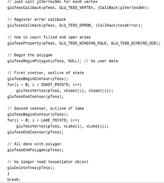
// Just call glVertex3dv for each vertex
gluTessCallback(pTess, GLU_TESS_VERTEX, (CallBack)glVertex3dv);
The GLU_TESS_BEGIN callback specifies the function to call at the beginning of each new primitive. Specifying glBegin simply tells the tessellator to call glBegin to begin a primitive batch. This may seem pointless, but you can also specify your own function here to do additional processing whenever a new primitive begins. For example, suppose you want to find out how many triangles are used in the final tessellated polygon.
The GLU_TESS_END callback, again, simply tells the tessellator to call glEnd and that you have no other specific code you want to inject into the process. Finally, the GLU_TESS_VERTEX call drops in a call to glVertex3dv to specify the tessellated vertex data. Tessellation requires that vertex data be specified as double precision, and always uses three component vertices. Again, you could substitute your own function here to do some additional processing (such as adding color, normal, or texture coordinate information).
If you’re wondering, CallBack is just a typedef defined in gltools.h to represent a generic function pointer for these functions.
For an example of specifying your own callback (instead of cheating and just using existing OpenGL functions), the following code shows the registration of a function to report any errors that may occur during tessellation:
////////////////////////////////////////////////////////////////////
// Tessellation error callback
void tessError(GLenum error)
{
// Get error message string
const char *szError = (const char *)gluErrorString(error);
// Set error message as window caption
glutSetWindowTitle(szError);
}
. . .
. . .
// Register error callback
gluTessCallback(pTess, GLU_TESS_ERROR, (CallBack)tessError);
Specifying Vertex Data
To begin a polygon (this corresponds to step 3 shown earlier), you call the following function:
void gluTessBeginPolygon(GLUTesselator *tobj, void *data);
You first pass in the tessellator object and then a pointer to any user-defined data that you want associated with this tessellation. This data can be sent back to you during tessellation using the callback functions listed for gluTessCallback. Often, this is just NULL. To finish the polygon (step 8) and begin tessellation, call this function:
void gluTessEndPolygon(GLUTesselator *tobj);
Nested within the beginning and ending of the polygon, you specify one or more contours using the following pair of functions (steps 4 and 6):
void gluTessBeginContour(GLUTesselator *tobj);
void gluTessEndContour(GLUTesselator *tobj);
Finally, within the contour, you must add the vertices that make up that contour (step 5). The following function feeds the vertices, one at a time, to the tessellator:
void gluTessVertex(GLUTesselator *tobj, GLdouble v[3], void *data);
The v parameter contains the actual vertex data used for tessellator calculations. The data parameter is a pointer to the vertex data passed to the callback function specified by GLU_VERTEX. Why two different arguments to specify the same thing? Because the pointer to the vertex data may also point to additional information about the vertex (color, normals, and so on). If you specify your own function for GLU_VERTEX (instead of our cheat), you can access this additional vertex data in the callback routine.
Putting It All Together
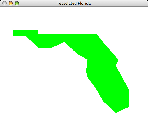
Now let’s look at an example that takes a complex polygon and performs tessellation to render a solid shape. The sample program FLORIDA contains the vertex information to draw the crude, but recognizable, shape of the state of Florida. The program has three modes of rendering, accessible via the context menu: Line Loops, Concave Polygon, and Complex Polygon. The basic shape with Line Loops is shown in Figure 10.23.
Figure 10.23. The basic outline of Florida.

Listing 10.5 shows the vertex data and the rendering code that draws the outlines for the state and Lake Okeechobee.
Listing 10.5. Vertex Data and Drawing Code for State Outline

For the Concave Polygon rendering mode, only the outside contour is drawn. This results in a solid filled shape, despite the fact that the polygon is clearly concave. This result is shown in Figure 10.24, and the tessellation code is shown in Listing 10.6.
Figure 10.24. A solid convex polygon.
Listing 10.6. Drawing a Convex Polygon

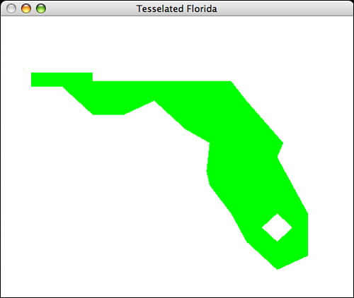
Finally, we present a more complex polygon, one with a hole in it. The Complex Polygon drawing mode draws the solid state, but with a hole representing Lake Okeechobee (a large lake in south Florida, typically shown on maps). The output is shown in Figure 10.25, and the relevant code is presented in Listing 10.7.
Figure 10.25. The solid polygon, but with a hole.
Listing 10.7. Tessellating a Complex Polygon with Multiple Contours

This code contained a new function call:
// How to count filled and open areas
gluTessProperty(pTess, GLU_TESS_WINDING_RULE, GLU_TESS_WINDING_ODD);
This call tells the tessellator how to decide what areas to fill in and which areas to leave empty when there are multiple contours. The value GLU_TESS_WINDING_ODD is actually the default, and we could have skipped this function. However, you should understand how the tessellator handles nested contours. By specifying ODD, we are saying that any given point inside the polygon is filled in if it is enclosed in an odd number of contours. The area inside the lake (inner contour) is surrounded by two (an even number) contours and is left unfilled. Points outside the lake but inside the state boundary are enclosed by only one contour (an odd number) and are drawn filled.
Summary
The quadrics library makes creating a few simple surfaces (spheres, cylinders, disks, and cones) child’s play. Expanding on this concept into more advanced curves and surfaces could have made this chapter the most intimidating in the entire book. As you have seen, however, the concepts behind these curves and surfaces are not very difficult to understand. Appendix A suggests further reading if you want in-depth mathematical information or tips on creating NURBS-based models.
Other examples from this chapter give you a good starting point for experimenting with NURBS. Adjust the control points and knot sequences to create warped or rumpled surfaces. Also, try some quadratic surfaces and some with higher order than the cubic surfaces. Watch out: One pitfall to avoid as you play with these curves is trying too hard to create one complex surface out of a single NURB. You can find greater power and flexibility if you compose complex surfaces out of several smaller and easy-to-handle NURBS or Bézier surfaces.
Finally, in this chapter, we saw OpenGL’s powerful support for automatic polygon tessellation. You learned that you can draw complex surfaces, shapes, and patterns with only a few points that specify the boundaries. You also learned that concave regions and even regions with holes can be broken down into simpler convex primitives using the GLU library’s tessellator object.
In the next chapter, you will learn about display lists. As you read that chapter, think about all the work that is being done under the covers to facilitate the power of these functions. Also think about the fact that most of the time, these functions are going to be used to draw static (unchanging) geometry. The techniques of the next chapter will allow you to dramatically increase the performance of what you have just learned here.