Chapter 6. More on Colors and Materials
WHAT YOU’LL LEARN IN THIS CHAPTER:

In the preceding chapter, you learned that there is more to making a ball appear red than just setting the drawing color to red. Material properties and lighting parameters can go a long way toward adding realism to your graphics, but modeling the real world has a few other challenges that we will address in this chapter. For starters, many effects are accomplished by means of blending colors together. Transparent objects such as stained-glass windows or plastic bottles allow you to see through them, but the light from the objects behind them is blended with the color of the transparent object you are seeing through. This type of transparency is achieved in OpenGL by drawing the background objects first and then blending the foreground object in front with the colors that are already present in the color buffer. A good part of making this technique work requires that we now consider the fourth color component that until now we have been ignoring, alpha.
Blending
You have already learned that OpenGL rendering places color values in the color buffer under normal circumstances. You have also learned that depth values for each fragment are also placed in the depth buffer. When depth testing is turned off (disabled), new color values simply overwrite any other values already present in the color buffer. When depth testing is turned on (enabled), new color fragments replace an existing fragment only if they are deemed closer to the near clipping plane than the values already there. Under normal circumstances then, any drawing operation is either discarded entirely, or just completely overwrites any old color values, depending on the result of the depth test. This obliteration of the underlying color values no longer happens the moment you turn on OpenGL blending:
glEnable(GL_BLEND);
When blending is enabled, the incoming color is combined with the color value already present in the color buffer. How these colors are combined leads to a great many and varied special effects.
Combining Colors
First, we must introduce a more official terminology for the color values coming in and already in the color buffer. The color value already stored in the color buffer is called the destination color, and this color value contains the three individual red, green, and blue components, and optionally a stored alpha value as well. A color value that is coming in as a result of more rendering commands that may or may not interact with the destination color is called the source color. The source color also contains either three or four color components (red, green, blue, and optionally alpha).
How the source and destination colors are combined when blending is enabled is controlled by the blending equation. By default, the blending equation looks like this:
Cf = (Cs * S) + (Cd * D)
Here, Cf is the final computed color, Cs is the source color, Cd is the destination color, and S and D are the source and destination blending factors. These blending factors are set with the following function:
glBlendFunc(GLenum S, GLenum D);
As you can see, S and D are enumerants and not physical values that you specify directly. Table 6.1 lists the possible values for the blending function. The subscripts stand for source, destination, and color (for blend color, to be discussed shortly). R, G, B, and A stand for Red, Green, Blue, and Alpha, respectively.
Table 6.1. OpenGL Blending Factors

Remember that colors are represented by floating-point numbers, so adding them, subtracting them, and even multiplying them are all perfectly valid operations. Table 6.1 may seem a bit bewildering, so let’s look at a common blending function combination:
glBlendFunc(GL_SRC_ALPHA, GL_ONE_MINUS_SRC_ALPHA);
This function tells OpenGL to take the source (incoming) color and multiply the color (the RGB values) by the alpha value. Add this to the result of multiplying the destination color by one minus the alpha value from the source. Say, for example, that you have the color Red (1.0f, 0.0f, 0.0f, 0.0f) already in the color buffer. This is the destination color, or Cd. If something is drawn over this with the color blue and an alpha of 0.6 (0.0f, 0.0f, 1.0f, 0.6f), you would compute the final color as shown here:
Cd = destination color = (1.0f, 0.0f, 0.0f, 0.0f)
Cs = source color = (0.0f, 0.0f, 1.0f, 0.6f)
S = source alpha = 0.6
D = one minus source alpha = 1.0 – 0.6 = 0.4
Now, the equation
Cf = (Cs * S) + (Cd * D)
evaluates to
Cf = (Blue * 0.6) + (Red * 0.4)
The final color is a scaled combination of the original red value and the incoming blue value. The higher the incoming alpha value, the more of the incoming color is added and the less of the original color is retained.
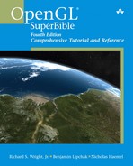
This blending function is often used to achieve the effect of drawing a transparent object in front of some other opaque object. This technique does require, however, that you draw the background object or objects first and then draw the transparent object blended over the top. The effect can be quite dramatic. For example, in the REFLECTION sample program, we will use transparency to achieve the illusion of a reflection in a mirrored surface. We begin with a rotating torus with a sphere revolving around it, similar to the view in the Sphere World example from Chapter 5, “Color, Materials, and Lighting: The Basics.” Beneath the torus and sphere, we will place a reflective tiled floor. The output from this program is shown in Figure 6.1, and the drawing code is shown in Listing 6.1.
Figure 6.1. Using blending to create a fake reflection effect.

Listing 6.1. Rendering Function for the REFLECTION Program
The basic algorithm for this effect is to draw the scene upside down first. We use one function to draw the scene, DrawWorld, but to draw it upside down, we scale by –1 to invert the y-axis, reverse our polygon winding, and place the light down beneath us. After drawing the upside-down world, we draw the ground, but we use blending to create a transparent floor over the top of the inverted world. Finally, we turn off blending, put the light back overhead, and draw the world right side up.
Changing the Blending Equation
The blending equation we showed you earlier,
Cf = (Cs * S) + (Cd * D)
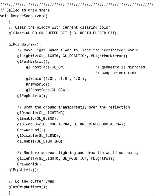
is the default blending equation. You can actually choose from five different blending equations, each given in Table 6.2 and selected with the following function:
void glBlendEquation(GLenum mode);
Table 6.2. Available Blend Equation Modes
In addition to glBlendFunc, you have even more flexibility with this function:
void glBlendFuncSeparate(GLenum srcRGB, GLenum dstRGB, GLenum srcAlpha,
GLenum dstAlpha);
Whereas glBlendFunc specifies the blend functions for source and destination RGBA values, glBlendFuncSeparate allows you to specify blending functions for the RGB and alpha components separately.
Finally, as shown in Table 6.1, the GL_CONSTANT_COLOR, GL_ONE_MINUS_CONSTANT_COLOR, GL_CONSTANT_ALPHA, and GL_ONE_MINUS_CONSTANT_ALPHA values all allow a constant blending color to be introduced to the blending equation. This constant blending color is initially black (0.0f, 0.0f, 0.0f, 0.0f), but it can be changed with this function:
void glBlendColor(GLclampf red, GLclampf green, Glclampf blue, GLclampf alpha);
Antialiasing
Another use for OpenGL’s blending capabilities is antialiasing. Under most circumstances, individual rendered fragments are mapped to individual pixels on a computer screen. These pixels are square (or squarish), and usually you can spot the division between two colors quite clearly. These jaggies, as they are often called, catch the eye’s attention and can destroy the illusion that the image is natural. These jaggies are a dead giveaway that the image is computer generated! For many rendering tasks, it is desirable to achieve as much realism as possible, particularly in games, simulations, or artistic endeavors. Figure 6.2 shows the output for the sample program SMOOTHER. In Figure 6.3, we have zoomed in on a line segment and some points to show the jagged edges.
Figure 6.2. Output from the program SMOOTHER.

Figure 6.3. A closer look at some jaggies.

To get rid of the jagged edges between primitives, OpenGL uses blending to blend the color of the fragment with the destination color of the pixel and its surrounding pixels. In essence, pixel colors are smeared slightly to neighboring pixels along the edges of any primitives.
Turning on antialiasing is simple. First, you must enable blending and set the blending function to be the same as you used in the preceding section for transparency:
glEnable(GL_BLEND);
glBlendFunc(GL_SRC_ALPHA, GL_ONE_MINUS_SRC_ALPHA);
You also need to make sure the blend equation is set to GL_ADD, but because this is the default and most common blending equation, we don’t show it here. After blending is enabled and the proper blending function and equation are selected, you can choose to antialias points, lines, and/or polygons (any solid primitive) by calling glEnable:
glEnable(GL_POINT_SMOOTH); // Smooth out points
glEnable(GL_LINE_SMOOTH); // Smooth out lines
glEnable(GL_POLYGON_SMOOTH); // Smooth out polygon edges
You should use GL_POLYGON_SMOOTH with care. You might expect to smooth out edges on solid geometry, but there are other tedious rules to making this work. For example, geometry that overlaps requires a different blending mode, and you may need to sort your scene from front to back. We won’t go into the details because this method of solid object antialiasing has fallen out of common use and has largely been replaced by a superior route to smoothing edges on 3D geometry called multisampling. This feature is discussed in the next section. Without multisampling, you can still get this overlapping geometry problem with antialiased lines that overlap. For wireframe rendering, for example, you can usually get away with just disabling depth testing to avoid the depth artifacts at the line intersections.
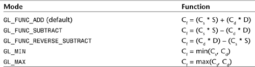
Listing 6.2 shows the code from the SMOOTHER program that responds to a pop-up menu that allows the user to switch between antialiased and non-antialiased rendering modes. When this program is run with antialiasing enabled, the points and lines appear smoother (fuzzier). In Figure 6.4, a zoomed-in section shows the same area as Figure 6.3, but now with the jagged edges smoothed out.

Listing 6.2. Switching Between Antialiased and Normal Rendering
Note especially here the calls to the glHint function discussed in Chapter 2, “Using OpenGL.” There are many algorithms and approaches to achieve antialiased primitives. Any specific OpenGL implementation may choose any one of those approaches, and perhaps even support two! You can ask OpenGL, if it does support multiple antialiasing algorithms, to choose one that is very fast (GL_FASTEST) or the one with the most accuracy in appearance (GL_NICEST).
Multisample
One of the biggest advantages to antialiasing is that it smoothes out the edges of primitives and can lend a more natural and realistic appearance to renderings. Point and line smoothing is widely supported, but unfortunately polygon smoothing is not available on all platforms. Even when GL_POLYGON_SMOOTH is available, it is not as convenient a means of having your whole scene antialiased as you might think. Because it is based on the blending operation, you would need to sort all your primitives from front to back! Yuck.
A more recent addition to OpenGL to address this shortcoming is multisampling. When this feature is supported (it is an OpenGL 1.3 feature), an additional buffer is added to the framebuffer that includes the color, depth, and stencil values. All primitives are sampled multiple times per pixel, and the results are stored in this buffer. These samples are resolved to a single value each time the pixel is updated, so from the programmer’s standpoint, it appears automatic and happens “behind the scenes.” Naturally, this extra memory and processing that must take place are not without their performance penalties, and some implementations may not support multisampling for multiple rendering contexts.
To get multisampling, you must first obtain a rendering context that has support for a multisampled framebuffer. This varies from platform to platform, but GLUT exposes a bit field (GLUT_MULTISAMPLE) that allows you to request this until you reach the operating system–specific chapters in Part III. For example, to request a multisampled, full-color, double-buffered frame buffer with depth, you would call
glutInitDisplayMode(GLUT_DOUBLE | GLUT_RGB | GLUT_DEPTH | GLUT_MULTISAMPLE);
You can turn multisampling on and off using the glEnable/glDisable combination and the GL_MULTISAMPLE token:
glEnable(GL_MULTISAMPLE);
or
glDisable(GL_MULTISAMPLE);
The sample program MULTISAMPLE is simply the Sphere World sample from the preceding chapter with multisampling selected and enabled. Figure 6.5 shows the difference between two zoomed-in sections from each program. You can see that multisampling really helps smooth out the geometry’s edges on the image to the right, lending to a much more pleasing appearance to the rendered output.
Figure 6.5. Zoomed-in view contrasting normal and multisampled rendering.
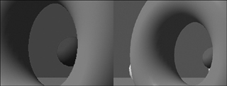
Another important note about multisampling is that when it is enabled, the point, line, and polygon smoothing features are ignored if enabled. This means you cannot use point and line smoothing at the same time as multisampling. On a given OpenGL implementation, points and lines may look better with smoothing turned on instead of multisampling. To accommodate this, you might turn off multisampling before drawing points and lines and then turn on multisampling for other solid geometry. The following pseudocode shows a rough outline of how to do this:
glDisable(GL_MULTISAMPLE);
glEnable(GL_POINT_SMOOTH);
// Draw some smooth points
// ...
glDisable(GL_POINT_SMOOTH);
glEnable(GL_MULTISAMPLE);
Of course if you do not have a multisampled buffer to begin with, OpenGL behaves as if GL_MULTISAMPLE were disabled.
The multisample buffers use the RGB values of fragments by default and do not include the alpha component of the colors. You can change this by calling glEnable with one of the following three values:
• GL_SAMPLE_ALPHA_TO_COVERAGE—Use the alpha value.
• GL_SAMPLE_ALPHA_TO_ONE—Set alpha to 1 and use it.
• GL_SAMPLE_COVERAGE—Use the value set with glSampleCoverage.
When GL_SAMPLE_COVERAGE is enabled, the glSampleCoverage function allows you to specify a specific value that is ANDed (bitwise) with the fragment coverage value:
void glSampleCoverage(GLclampf value, GLboolean invert);
This fine-tuning of how the multisample operation works is not strictly specified by the specification, and the exact results may vary from implementation to implementation.
Applying Fog
Another easy-to-use special effect that OpenGL supports is fog. With fog, OpenGL blends a fog color that you specify with geometry after all other color computations have been completed. The amount of the fog color mixed with the geometry varies with the distance of the geometry from the camera origin. The result is a 3D scene that appears to contain fog. Fog can be useful for slowly obscuring objects as they “disappear” into the background fog; or a slight amount of fog will produce a hazy effect on distant objects, providing a powerful and realistic depth cue. Figure 6.6 shows output from the sample program FOGGED. As you can see, this is nothing more than the ubiquitous Sphere World example with fog turned on.
Figure 6.6. Sphere World with fog.

Listing 6.3 shows the few lines of code added to the SetupRC function to produce this effect.
Listing 6.3. Setting Up Fog for Sphere World
// Grayish background
glClearColor(fLowLight[0], fLowLight[1], fLowLight[2], fLowLight[3]);
// Set up Fog parameters
glEnable(GL_FOG); // Turn Fog on
glFogfv(GL_FOG_COLOR, fLowLight); // Set fog color to match background
glFogf(GL_FOG_START, 5.0f); // How far away does the fog start
glFogf(GL_FOG_END, 30.0f); // How far away does the fog stop
glFogi(GL_FOG_MODE, GL_LINEAR); // Which fog equation to use
Turning fog on and off is as easy as using the following functions:
glEnable/glDisable(GL_FOG);
The means of changing fog parameters (how the fog behaves) is to use the glFog function. There are several variations on glFog:
void glFogi(GLenum pname, GLint param);
void glFogf(GLenum pname, GLfloat param);
void glFogiv(GLenum pname, GLint* params);
void glFogfv(GLenum pname, GLfloat* params);
The first use of glFog shown here is
glFogfv(GL_FOG_COLOR, fLowLight); // Set fog color to match background
When used with the GL_FOG_COLOR parameter, this function expects a pointer to an array of floating-point values that specifies what color the fog should be. Here, we used the same color for the fog as the background clear color. If the fog color does not match the background (there is no strict requirement for this), as objects become fogged, they will become a fog-colored silhouette against the background.
The next two lines allow us to specify how far away an object must be before fog is applied and how far away the object must be for the fog to be fully applied (where the object is completely the fog color):
glFogf(GL_FOG_START, 5.0f); // How far away does the fog start
glFogf(GL_FOG_END, 30.0f); // How far away does the fog stop
The parameter GL_FOG_START specifies how far away from the eye fogging begins to take effect, and GL_FOG_END is the distance from the eye where the fog color completely overpowers the color of the object. The transition from start to end is controlled by the fog equation, which we set to GL_LINEAR here:
glFogi(GL_FOG_MODE, GL_LINEAR); // Which fog equation to use
Fog Equations
The fog equation calculates a fog factor that varies from 0 to 1 as the distance of the fragment moves between the start and end distances. OpenGL supports three fog equations: GL_LINEAR, GL_EXP, and GL_EXP2. These equations are shown in Table 6.3.
Table 6.3. Three OpenGL Supported Fog Equations

In these equations, c is the distance of the fragment from the eye plane, end is the GL_FOG_END distance, and start is the GL_FOG_START distance. The value d is the fog density. Fog density is typically set with glFogf:
glFogf(GL_FOG_DENSITY, 0.5f);
Note that GL_FOG_START and GL_FOG_END only have an effect on GL_LINEAR fog. Figure 6.7 shows graphically how the fog equation and fog density parameters affect the transition from the original fragment color to the fog color. GL_LINEAR is a straight linear progression, whereas the GL_EXP and GL_EXP2 equations show two characteristic curves for their transitions. The fog density value has no effect with linear fog (GL_LINEAR), but the other two curves you see here are generally pulled downward with increasing density values. These graphs, for example, show approximately a density value of 0.5.
Figure 6.7. Fog density equations.

The distance to a fragment from the eye plane can be calculated in one of two ways. Some implementations (notably NVIDIA hardware) will use the actual fragment depth. Other implementations (notably many ATI chipsets) use the vertex distance and interpolate between vertices. The former method is sometimes referred to as fragment fog; and the later, vertex fog. Fragment fog requires more work than vertex fog, but often has a higher quality appearance. Both of the previously mentioned implementations honor the glHint parameter GL_FOG_HINT. To explicitly request fragment fog (better looking, but more work), call
glHint(GL_FOG_HINT, GL_NICEST);
For faster, less precise fog, you’d call
glHint(GL_FOG_HINT, GL_FASTEST);
Remember that hints are implementation dependent, may change over time, and are not required to be acknowledged or used by the driver at all. Indeed, you can’t even rely on which fog method will be the default!
Fog Coordinates
Rather than letting OpenGL calculate fog distance for you, you can actually do this yourself. This value is called the fog coordinate and can be set manually with the function glFogCoordf:
void glFogCoordf(Glfloat fFogDistance);
Fog coordinates are ignored unless you change the fog coordinate source with this function call:
glFogi(GL_FOG_COORD_SRC, GL_FOG_COORD); // use glFogCoord1f
To return to OpenGL-derived fog values, change the last parameter to GL_FRAGMENT_DEPTH:
glFogi(GL_FOG_COORD_SRC, GL_FRAGMENT_DEPTH);
This fog coordinate when specified is used as the fog distance in the equations of Table 6.3. Specifying your own fog distance allows you to change the way distance is calculated. For example, you may want elevation to play a role, lending to volumetric fog effects.
Accumulation Buffer
In addition to the color, stencil, and depth buffers, OpenGL supports what is called the accumulation buffer. This buffer allows you to render to the color buffer, and then instead of displaying the results in the window, copy the contents of the color buffer to the accumulation buffer. Several supported copy operations allow you to repeatedly blend, in different ways, the color buffer contents with the accumulated contents in the accumulation buffer (thus its name). When you have finished accumulating an image, you can then copy the accumulation buffer back to the color buffer and display the results with a buffer swap.
The behavior of the accumulation buffer is controlled by one function:
void glAccum(GLenumm op, GLfloat value);
The first parameter specifies which accumulation operation you want to use, and the second is a floating-point value used to scale the operation. Table 6.4 lists the accumulation operations supported.
Table 6.4. OpenGL Accumulation Operations

Because of the large amount of memory that must be copied and processed for accumulation buffer operations, few real-time applications make use of this capability. For non-real-time rendering, OpenGL can produce some astonishing effects that you might not expect from a real-time API. For example, you can render a scene multiple times and move the point of view around by a fraction of a pixel each time. Accumulating these multiple rendering passes blurs the sharp edges and can produce an entire scene fully antialiased with a quality that surpasses anything that can be done with multisampling. You can also use this blurring effect to blur the background or foreground of an image and then render the object of focus clearly afterward, simulating some depth-of-field camera effects.
In our sample program MOTIONBLUR, we will demonstrate yet another use of the accumulation buffer to create what appears to be a motion blur effect. A moving sphere is drawn repeatedly in different positions. Each time it is drawn, it is accumulated to the accumulation buffer, with a smaller weight on subsequent passes. The result is a brighter red sphere with a ghostlike image of itself following along behind. The output from this program is shown in Figure 6.8.
Figure 6.8. A motion-blurred flying sphere.

Listing 6.4 shows the DrawGeometry function, which draws all the geometry of the scene. The RenderScene function then repeatedly calls this function and accumulates the results into the accumulation buffer. When that process is finished, the lines
glAccum(GL_RETURN, 1.0f);
glutSwapBuffers();
copy the accumulation buffer back to the color buffer and perform the buffer swap.
Listing 6.4. Using the Accumulation Buffer for Motion Blur


Finally, you must remember to ask for an accumulation buffer when you set up your OpenGL rendering context (see the OS-specific chapters in Part III for how to perform this task on your platform). GLUT also provides support for the accumulation buffer by passing the token GLUT_ACCUM to the glutInitDisplayMode function, as shown here:
glutInitDisplayMode(GLUT_DOUBLE | GLUT_RGB | GLUT_DEPTH | GLUT_ACCUM);
Other Color Operations
Blending is a powerful OpenGL feature that enables a myriad of special effects algorithms. Aside from direct support for blending, fog, and an accumulation buffer, OpenGL also supports some other means of tweaking color values and fragments as they are written to the color buffer.
Color Masking
After a final color is computed, when it is about to be written to the color buffer, OpenGL allows you to mask out one or more of the color channels with the glColorMask function:
void glColorMask(GLboolean red, GLboolean green, GLboolean blue,
GLboolean alpha);
The parameters are for the red, green, blue, and alpha channels, respectively. Passing GL_TRUE allows writing of this channel, and GL_FALSE prevents writing to this channel.
Color Logical Operations
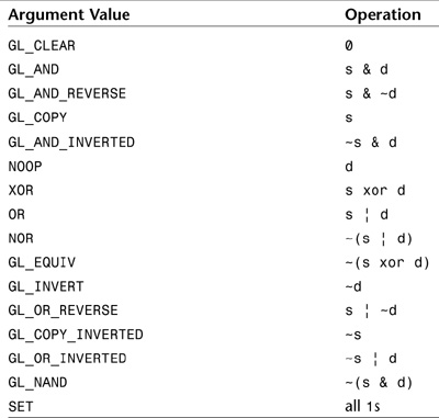
Many 2D graphics APIs allow binary logical operations to be performed between the source and the destination colors. OpenGL also supports these types of 2D operations with the glLogicOp function:
void glLogicOp(GLenum op);
The logical operation modes are listed in Table 6.5. The logical operation is not enabled by default and is controlled, as most states are, with glEnable/glDisable using the value GL_COLOR_LOGIC_OP. For example, to turn on the logical operations, you use the following:
glEnable(GL_COLOR_LOGIC_OP);
Table 6.5. Bitwise Color Logical Operations
Alpha Testing
Alpha testing allows you to tell OpenGL to discard incoming fragments whose alpha value fails the alpha comparison test. Discarded fragments are not written to the color, depth, stencil, or accumulation buffers. This feature allows you to improve performance by dropping values that otherwise might be written to the buffers and to eliminate geometry from the depth buffer that may not be visible in the color buffer (because of very low alpha values). The alpha test value and comparison function are specified with the glAlphaFunc function:
void glAlphaFunc(GLenum func, GLclampf ref);
The reference value is clamped to the range 0.0 to 1.0, and the comparison function may be specified by any of the constants in Table 6.6. You can turn alpha testing on and off with glEnable/glDisable using the constant GL_ALPHA_TEST. The behavior of this function is similar to the glDepthFunc function (see Appendix C, “API Reference”).
Table 6.6. Alpha Test Comparison Functions

Dithering
Dithering is a simple operation (in principle) that allows a display system with a small number of discrete colors to simulate displaying a much wider range of colors. For example, the color gray can be simulated by displaying a mix of white and black dots on the screen. More white than black dots make for a lighter gray, whereas more black dots make a darker gray. When your eye is far enough from the display, you cannot see the individual dots, and the blending effect creates the illusion of the color mix. This technique is useful for display systems that support only 8 or 16 bits of color information. Each OpenGL implementation is free to implement its own dithering algorithm, but the effect can be dramatically improved image quality on lower-end color systems. By default, dithering is turned on, and it can be controlled with glEnable/glDisable and the constant GL_DITHER:
glEnable(GL_DITHER); // Initially enabled
On higher-end display systems with greater color resolution, the implementation may not need dithering, and dithering may not be employed at a potentially considerable performance savings.
Summary
In this chapter, we took color beyond simple shading and lighting effects. You saw how to use blending to create transparent and reflective surfaces and create antialiased points, lines, and polygons with the blending and multisampling features of OpenGL. You also were introduced to the accumulation buffer and saw at least one common special effect that it is normally used for. Finally, you saw how OpenGL supports other color manipulation features such as color masks, bitwise color operations, and dithering, and how to use the alpha test to discard fragments altogether. Now we progress further in the next chapter from colors, shading, and blending to operations that incorporate real image data.
Included in the source distribution for this chapter, you’ll find an update of the Sphere World example from Chapter 5. You can study the source code to see how we have incorporated many of the techniques from this chapter to add some additional depth queuing to the world with fog, partially transparent shadows on the ground, and fully antialiased rendering of all geometry.