
Chapter 11. It’s All About the Pipeline: Faster Geometry Throughput
WHAT YOU’LL LEARN IN THIS CHAPTER:

In the preceding chapters, we have covered most of the basic OpenGL rendering techniques and technologies. With this knowledge, there are few 3D scenes you can envision that cannot be realized using only the first half of this book. Getting a detailed image onscreen, however, must often be balanced with the competing goal of performance. For some applications it may be perfectly acceptable to wait for several seconds or even minutes for a completed image to be rendered. For most real-time applications, however, the goal is usually to render a completed and usually dynamic scene many dozens of times per second!
A common hindrance to high performance in real-time applications is geometry throughput. Modern scenes and models are composed of many thousands of vertices, often accompanied by normals, texture coordinates, and other attributes. This is a lot of data that must be operated on by both the CPU and the GPU. In addition, just moving the data from the application to the graphics hardware can be a substantial performance bottleneck.
This chapter focuses exclusively on these issues. OpenGL contains a number of features that allow the programmer a great deal of flexibility and convenience when dealing with the goal of fast geometry throughput, each with its own advantages and disadvantages in terms of speed, flexibility, and ease of use.
Display Lists
So far, all of our primitive batches have been assembled using glBegin/glEnd pairs with individual glVertex calls between them. This is a very flexible means of assembling a batch of primitives, and is incredibly easy to use and understand. Unfortunately, when performance is taken into account, it is also the worst possible way to submit geometry to graphics hardware. Consider the following pseudocode to draw a single lit textured triangle:
glBegin(GL_TRIANGLES);
glNormal3f(x, y, z);
glTexCoord2f(s, t);
glVertex3f(x, y, z);
glNormal3f(x, y, z);
glTexCoord2f(s, t);
glVertex3f(x, y, z);
glNormal3f(x, y, z);
glTexCoord2f(s, t);
glVertex3f(x, y, z);
glEnd();
For a single triangle, that’s 11 function calls. Each of these functions contains potentially expensive validation code in the OpenGL driver. In addition, we must pass 24 different four byte parameters (one at a time!) pushed on the stack, and of course return to the calling function. That’s a good bit of work for the CPU to perform to draw a single triangle. Now, multiply this by a 3D scene containing 10,000 or more triangles, and it is easy to imagine the graphics hardware sitting idle waiting on the CPU to assemble and submit geometry batches. There are some strategies that will soften the blow, of course. You can use vector-based functions such as glVertex3fv, you can consolidate batches, and you can use strips and fans to reduce redundant transformations and copies. However, the basic approach is flawed from a performance standpoint because it requires many thousands of very small, potentially expensive operations to submit a batch of geometry. This method of submitting geometry batches is often called immediate mode rendering. Let’s look at how OpenGL processes this data and see how there is an opportunity to dramatically improve this situation.
Batch Processing
OpenGL has been described as a software interface to graphics hardware. As such, you might imagine that OpenGL commands are somehow converted into some specific hardware commands or operators by the driver and then sent on to the graphics card for immediate execution. If so, you would be mostly correct. Most OpenGL rendering commands are, in fact, converted into some hardware-specific commands, but these commands are not dispatched immediately to the hardware. Instead, they are accumulated in a local buffer until some threshold is reached, at which point they are flushed to the hardware.
The primary reason for this type of arrangement is that trips to the graphics hardware take a long time, at least in terms of computer time. To a human being, this process might take place very quickly, but to a CPU running at many billions of cycles per second, this is like waiting for a cruise ship to sail from North America to Europe and back. You certainly would not put a single person on a ship and wait for the ship to return before loading up the next person. If you have many people to send to Europe, you are going to cram as many people on the ship as you can! This analogy is very accurate: It is faster to send a large amount of data (within some limits) over the system bus to hardware all at once than to break it down into many bursts of smaller packages.
Keeping to the analogy, you also do not have to wait for the first cruise ship to return before you can begin filling the next ship with passengers. Sending the buffer to the graphics hardware (a process called flushing) is an asynchronous operation. This means that the CPU can move on to other tasks and does not have to wait for the batch of rendering commands just sent to be completed. You can literally have the hardware rendering a given set of commands while the CPU is busy calling a new set of commands for the next graphics image (typically called a frame when you’re creating an animation). This type of parallelization between the graphics hardware and the host CPU is highly efficient and often sought after by performance-conscious programmers.
Three events trigger a flush of the current batch of rendering commands. The first occurs when the driver’s command buffer is full. You do not have access to this buffer, nor do you have any control over the size of the buffer. The hardware vendors work hard to tune the size and other characteristics of this buffer to work well with their devices. A flush also occurs when you execute a buffer swap. The buffer swap cannot occur until all pending commands have been executed (you want to see what you have drawn!), so the flush is initiated, followed by the command to perform the buffer swap. A buffer swap is an obvious indicator to the driver that you are done with a given scene and that all commands should be rendered. However, if you are doing single-buffered rendering, OpenGL has no real way of knowing when you’re done sending commands and thus when to send the batch of commands to the hardware for execution. To facilitate this process, you can call the following function to manually trigger a flush:
void glFlush(void);
Some OpenGL commands, however, are not buffered for later execution—for example, glReadPixels and glDrawPixels. These functions directly access the framebuffer and read or write data directly. These functions actually introduce a pipeline stall, because the currently queued commands must be flushed and executed before you make direct changes to the color buffer. You can forcibly flush the command buffer, and wait for the graphics hardware to complete all its rendering tasks by calling the following function:
void glFinish(void);
This function is rarely used in practice. Typically this is for platform-specific requirements such as multithreading or multicontext rendering.
Preprocessed Batches
The work done every time you call an OpenGL command is not inconsequential. Commands are compiled, or converted, from OpenGL’s high-level command language into low-level hardware commands understood by the hardware. For complex geometry, or just large amounts of vertex data, this process is performed many thousands of times, just to draw a single image onscreen. This is, of course, the aforementioned problem with immediate mode rendering. How does our new knowledge of the command buffer help with this situation?
Often, the geometry or other OpenGL data remains the same from frame to frame. For example, a spinning torus is always composed of the same set of triangle strips, with the same vertex data, recalculated with expensive trigonometric functions every frame. The only thing changing frame to frame is the modelview matrix.
A solution to this needlessly repeated overhead is to save a chunk of precomputed data from the command buffer that performs some repetitive rendering task, such as drawing the torus. This chunk of data can later be copied back to the command buffer all at once, saving the many function calls and compilation work done to create the data.
OpenGL provides a facility to create a preprocessed set of OpenGL commands (the chunk of data) that can then be quickly copied to the command buffer for more rapid execution. This precompiled list of commands is called a display list, and creating one or more of them is an easy and straightforward process. Just as you delimit an OpenGL primitive with glBegin/glEnd, you delimit a display list with glNewList/glEndList. A display list, however, is named with an integer value that you supply. The following code fragment represents a typical example of display list creation:
glNewList(<unsigned integer name>,GL_COMPILE);
...
...
// Some OpenGL Code
...
...
glEndList();
The named display list now contains all OpenGL rendering commands that occur between the glNewList and glEndList function calls. The GL_COMPILE parameter tells OpenGL to compile the list but not to execute it yet. You can also specify GL_COMPILE_AND_EXECUTE to simultaneously build the display list and execute the rendering instructions. Typically, however, display lists are built (GL_COMPILE only) during program initialization and then executed later during rendering.
The display list name can be any unsigned integer. However, if you use the same value twice, the second display list overwrites the previous one. For this reason, it is convenient to have some sort of mechanism to keep you from reusing the same display list more than once. This is especially helpful when you are incorporating libraries of code written by someone else who may have incorporated display lists and may have chosen the same display list names.
OpenGL provides built-in support for allocating unique display list names. The following function returns the first of a series of display list integers that are unique:
GLuint glGenLists(GLsizei range);
The display list names are reserved sequentially, with the first name being returned by the function. You can call this function as often as you want and for as many display list names at a time as you may need. A corresponding function frees display list names and releases any memory allocated for those display lists:
void glDeleteLists(GLuint list, GLsizei range);
A display list, containing any number of precompiled OpenGL commands, is then executed with a single command:
void glCallList(GLuint list);
You can also execute a whole array of display lists with this command:
void glCallLists(GLsizei n, GLenum type, const GLvoid *lists);
The first parameter specifies the number of display lists contained by the array lists. The second parameter contains the data type of the array; typically, it is GL_UNSIGNED_BYTE. Conveniently, it is used very often as an offset to address font display lists.
Display List Caveats
A few important points about display lists are worth mentioning here. Although on most implementations, a display list should improve performance, your mileage may vary depending on the amount of effort the vendor puts into optimizing display list creation and execution. It is rare, however, for display lists not to offer a noticeable boost in performance, and they are widely relied on in applications that use OpenGL.
Display lists are typically good at creating precompiled lists of OpenGL commands, especially if the list contains state changes (turning lighting on and off, for example). If you do not create a display list name with glGenLists first, you might get a working display list on some implementations, but not on others. Some commands simply do not make sense in a display list. For example, reading the framebuffer into a pointer with glReadPixels makes no sense in a display list. Likewise, calls to glTexImage2D would store the original image data in the display list, followed by the command to load the image data as a texture. Basically, your textures stored this way would take up twice as much memory! Display lists excel, however, at precompiled lists of static geometry, with texture objects bound either inside or outside the display lists. Finally, display lists cannot contain calls that create display lists. You can have one display list call another, but you cannot put calls to glNewLists/glEndList inside a display list.
Converting to Display Lists
To demonstrate how easy it is to use display lists, and the potential for performance improvement, we have converted the Sphere World sample program to optionally use display lists (see the Sphere World sample program for this chapter). You can select with/without display lists via a context menu available via the right mouse button. We have also added a display to the window caption that displays the frame rate achieved using these two methods.
Converting the Sphere World sample to use display lists requires only a few additional lines of code. First, we add three variables that contain the display list identifiers for the three pieces of static geometry: a sphere, the ground, and the torus.
// Display list identifiers
GLuint sphereList, groundList, torusList;
Then, in the SetupRC function, we request three display list names and assign them to our display list variables:
// Get Display list names
groundList = glGenLists(3);
sphereList = groundList + 1;
torusList = groundList + 2;
Next, we add the code to generate the three display lists. Each display list simply calls the function that draws that piece of geometry:
// Prebuild the display lists
glNewList(sphereList, GL_COMPILE);
gltDrawSphere(0.1f, 40, 20);
glEndList();
// Create torus display list
glNewList(torusList, GL_COMPILE);
gltDrawTorus(0.35, 0.15, 61, 37);
glEndList();
// Create the ground display list
glNewList(groundList, GL_COMPILE);
DrawGround();
glEndList();
Finally, when drawing the objects, we select either the display list or the direct rendering method based on a flag set by the menu handler. For example, rendering a single sphere becomes this:
if(iMethod == 0)
gltDrawSphere(0.1f, 40, 20);
else
glCallList(sphereList);
Switching to display lists can have an amazing impact on performance. Some OpenGL implementations even try to store display lists in memory on the graphics hardware directly if possible, further reducing the work required to get the data to the graphics processor. Figure 11.1 shows the new improved SPHEREWORLD sample running with display lists activated. Without display lists on the Macintosh this was written on, the frame rate was about 50 fps. With display lists, the frame rate shoots up to over 300!
Figure 11.1. SPHEREWORLD with display lists.

Why should you care about rendering performance? The faster and more efficient your rendering code, the more visual complexity you can add to your scene without dragging down the frame rate too much. Higher frame rates yield smoother and better-looking animations. You can also use the extra CPU time to perform other tasks such as physics calculations or lengthy I/O operations on a separate thread.
Vertex Arrays
Display lists are a frequently used and convenient means of precompiling sets of OpenGL commands. In our previous example, the many spheres required a great deal of trigonometric calculations that were saved when we placed the geometry in display lists. You might consider that we could just as easily have created some arrays to store the vertex data for the models and thus saved all the computation time just as easily as with the display lists.
You might be right about this way of thinking—to a point. Some implementations store display lists more efficiently than others, and if all you’re really compiling is the vertex data, you can simply place the model’s data in one or more arrays and render from the array of precalculated geometry. The only drawback to this approach is that you must still loop through the entire array moving data to OpenGL one vertex at a time. Depending on the amount of geometry involved, taking this approach could incur a substantial performance penalty. The advantage, however, is that, unlike with display lists, the geometry does not have to be static. Each time you prepare to render the geometry, some function could be applied to all the geometry data and perhaps displace or modify it in some way. For example, say a mesh used to render the surface of an ocean could have rippling waves moving across the surface. A swimming whale or jellyfish could also be cleverly modeled with deformable meshes in this way.
With OpenGL, you can, in fact, have the best of both scenarios by using vertex arrays. With vertex arrays, you can precalculate or modify your geometry on the fly but do a bulk transfer of all the geometry data at one time. Basic vertex arrays can be almost as fast as display lists, but without the requirement that the geometry be static. It might also simply be more convenient to store your data in arrays for other reasons and thus also render directly from the same arrays (this approach could also potentially be more memory efficient).
Using vertex arrays in OpenGL involves four basic steps. First, you must assemble your geometry data in one or more arrays. You can do this algorithmically or perhaps by loading the data from a disk file. Second, you must tell OpenGL where the data is. When rendering is performed, OpenGL pulls the vertex data directly from the arrays you have specified. Third, you must explicitly tell OpenGL which arrays you are using. You can have separate arrays for vertices, normals, colors, and so on, and you must let OpenGL know which of these data sets you want to use. Finally, you execute the OpenGL commands to actually perform the rendering using your vertex data.
To demonstrate these four steps, we revisit an old sample from another chapter. We’ve rewritten the POINTSPRITE sample from Chapter 9, “Texture Mapping: Beyond the Basics,” for the STARRYNIGHT sample in this chapter. The STARRYNIGHT sample creates three arrays (for three different-sized stars) that contain randomly initialized positions for stars in a starry sky. We then use vertex arrays to render directly from these arrays, bypassing the glBegin/glEnd mechanism entirely. Figure 11.2 shows the output of the STARRYNIGHT sample program, and Listing 11.1 shows the important portions of the source code.
Figure 11.2. Output from the STARRYNIGHT program.

Listing 11.1. Setup and Rendering Code for the STARRYNIGHT Sample


Loading the Geometry
The first prerequisite to using vertex arrays is that your geometry must be stored in arrays. In Listing 11.1, you see three globally accessible arrays of two-dimensional vectors. They contain x and y coordinate locations for the three groups of stars:
// Array of small stars
#define SMALL_STARS 100
M3DVector2f vSmallStars[SMALL_STARS];
#define MEDIUM_STARS 40
M3DVector2f vMediumStars[MEDIUM_STARS];
#define LARGE_STARS 15
M3DVector2f vLargeStars[LARGE_STARS];
Recall that this sample program uses an orthographic projection and draws the stars as points at random screen locations. Each array is populated in the SetupRC function with a simple loop that picks random x and y values that fall within the portion of the window we want the stars to occupy. The following few lines from the listing show how just the small star list is populated:
// Populate star list
for(i = 0; i < SMALL_STARS; i++)
{
vSmallStars[i][0] = (GLfloat)(rand() % SCREEN_X);
vSmallStars[i][1] = (GLfloat)(rand() % (SCREEN_Y - 100))+100.0f;
}
Enabling Arrays
In the RenderScene function, we enable the use of an array of vertices with the following code:
// Using vertex arrays
glEnableClientState(GL_VERTEX_ARRAY);
This is the first new function for using vertex arrays, and it has a corresponding disabling function:
void glEnableClientState(GLenum array);
void glDisableClientState(GLenum array);
These functions accept the following constants, turning on and off the corresponding array usage: GL_VERTEX_ARRAY, GL_COLOR_ARRAY, GL_SECONDARY_COLOR_ARRAY, GL_NORMAL_ARRAY, GL_FOG_COORDINATE_ARRAY, GL_TEXURE_COORD_ARRAY, and GL_EDGE_FLAG_ARRAY. For our STARRYNIGHT example, we are sending down only a list of vertices. As you can see, you can also send down a corresponding array of normals, texture coordinates, colors, and so on.
Here’s one question that commonly arises with the introduction of this function: Why did the OpenGL designers add a new glEnableClientState function instead of just sticking with glEnable? A good question. The reason has to do with how OpenGL is designed to operate. OpenGL was designed using a client/server model. The server is the graphics hardware, and the client is the host CPU and memory. On the PC, for example, the server would be the graphics card, and the client would be the PC’s CPU and main memory. Because this state of enabled/disabled capability specifically applies to the client side of the picture, a new set of functions was derived.
Where’s the Data?
Before we can actually use the vertex data, we must still tell OpenGL where the data is stored. The following single line in the STARRYNIGHT example does this:
glVertexPointer(2, GL_FLOAT, 0, vSmallStars);
Here, we find our next new function. The glVertexPointer function tells OpenGL where the vertex data is stored. There are also corresponding functions for the other types of vertex array data:
void glVertexPointer(GLint size, GLenum type, GLsizei stride,
const void *pointer);
void glColorPointer(GLint size, GLenum type, GLsizei stride,
const void *pointer);
void glTexCoordPointer(GLint size, GLenum type, GLsizei stride,
const void *pointer);
void glSecondaryColorPointer(GLint size, GLenum type, GLsizei stride,
const void *pointer);
void glNormalPointer(GLenum type, GLsizei stride, const void *pData);
void glFogCoordPointer(GLenum type, GLsizei stride, const void *pointer);
void glEdgeFlagPointer(GLenum type, GLsizei stride, const void *pointer);
These functions are all closely related and take nearly identical arguments. All but the normal, fog coordinate, and edge flag functions take a size argument first. This argument tells OpenGL the number of elements that make up the coordinate type. For example, vertices can consist of two (x,y), three (x,y,z), or four (x,y,z,w) components. Normals, however, are always three components, and fog coordinates and edge flags are always one component; thus, it would be redundant to specify the argument for these functions.
The type parameter specifies the OpenGL data type for the array. Not all data types are valid for all vertex array specifications. Table 11.1 lists the seven vertex array functions (index pointers are used for color index mode and are thus excluded here) and the valid data types that can be specified for the data elements.
Table 11.1. Valid Vertex Array Sizes and Data Types

The stride parameter specifies the space in bytes between each array element. Typically, this value is just 0, and array elements have no data gaps between values. Finally, the last parameter is a pointer to the array of data. For arrays, this is simply the name of the array.
This leaves us a little in the dark concerning multitexture. When using the glBegin/glEnd paradigm, we learned a new function for sending texture coordinates for each texture unit, called glMultiTexCoord. When using vertex arrays, you can change the target texture unit for glTexCoordPointer with this function:
glClientActiveTexture(GLenum texture);
Here the target parameter is GL_TEXTURE0, GL_TEXTURE1, and so forth.
Pull the Data and Draw
Finally, we’re ready to render using our vertex arrays. We can actually use the vertex arrays in two different ways. For illustration, first look at the nonvertex array method that simply loops through the array and passes a pointer to each array element to glVertex:
glBegin(GL_POINTS);
for(i = 0; i < SMALL_STARS; i++)
glVertex2fv(vSmallStars[i]);
glEnd();
Because OpenGL now knows about our vertex data, we can have OpenGL look up the vertex values for us with the following code:
glBegin(GL_POINTS);
for(i = 0; i < SMALL_STARS; i++)
glArrayElement(i);
glEnd();
The glArrayElement function looks up the corresponding array data from any arrays that have been enabled with glEnableClientState. If an array has been enabled, and a corresponding array has not been specified (glVertexPointer, glColorPointer, and so on), an illegal memory access will likely cause the program to crash. The advantage to using glArrayElement is that a single function call can now replace several function calls (glNormal, glColor, glVertex, and so forth) needed to specify all the data for a specific vertex. Sometimes you might want to jump around in the array in nonsequential order as well.
Most of the time, however, you will find that you are simply transferring a block of vertex data that needs to be traversed from beginning to end. In these cases (as is the case with the STARRYNIGHT sample), OpenGL can transfer a single block of any enabled arrays with a single function call:
void glDrawArrays(GLenum mode, GLint first, GLint count);
In this function, mode specifies the primitive to be rendered (one primitive batch per function call). The first parameter specifies where in the enabled arrays to begin retrieving data, and the count parameter tells how many array elements to retrieve. In the case of the STARRYNIGHT example, we rendered the array of small stars as follows:
glDrawArrays(GL_POINTS, 0, SMALL_STARS);
OpenGL implementations can optimize these block transfers, resulting in significant performance gains over multiple calls to the individual vertex functions such as glVertex and glNormal.
Indexed Vertex Arrays
Indexed vertex arrays are vertex arrays that are not traversed in order from beginning to end, but are traversed in an order that is specified by a separate array of index values. This may seem a bit convoluted, but actually indexed vertex arrays can save memory and reduce transformation overhead. Under ideal conditions, they can actually be faster than display lists!
The reason for this extra efficiency is that the array of vertices can be smaller than the array of indices. Adjoining primitives such as triangles can share vertices in ways not possible by just using triangle strips or fans. For example, using ordinary rendering methods or vertex arrays, there is no other mechanism to share a set of vertices between two adjacent triangle strips. Figure 11.3 shows two triangle strips that share one edge.
Figure 11.3. Two triangle strips in which the vertices share an edge.

Although triangle strips make good use of shared vertices between triangles in the strip, there is no way to avoid the overhead of transforming the vertices shared between the two strips because each strip must be specified individually.
Now let’s look at a simple example; then we’ll look at a more complex model and examine the potential savings of using indexed arrays.
A Simple Cube
We can save a considerable amount of memory if we can reuse a normal or vertex in a vertex array without having to store it more than once. Not only is memory saved, but also a good OpenGL implementation is optimized to transform these vertices only once, saving valuable transformation time.
Instead of creating a vertex array containing all the vertices for a given geometric object, you can create an array containing only the unique vertices for the object. Then you can use another array of index values to specify the geometry. These indices reference the vertex values in the first array. Figure 11.4 shows this relationship.
Figure 11.4. An index array referencing an array of unique vertices.

Each vertex consists of three floating-point values, but each index is only an integer value. A float and an integer are 4 bytes on most machines, which means you save 8 bytes for each reused vertex for the cost of 4 extra bytes for every vertex. For a small number of vertices, the savings might not be great; in fact, you might even use more memory using an indexed array than you would have by just repeating vertex information. For larger models, however, the savings can be substantial.
Figure 11.5 shows a cube with each vertex numbered. For our next sample program, CUBEDX, we create a cube using indexed vertex arrays.
Figure 11.5. A cube containing eight unique numbered vertices.

Listing 11.2 shows the code from the CUBEDX program to render the cube using indexed vertex arrays. The eight unique vertices are in the corners array, and the indices are in the indexes array. In RenderScene, we set the polygon mode to GL_LINE so that the cube is wireframed.
Listing 11.2. Code from the CUBEDX Program to Use Indexed Vertex Arrays

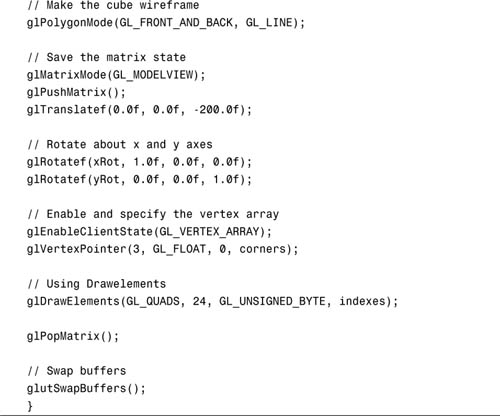
OpenGL has native support for indexed vertex arrays, as shown in the glDrawElements function. The key line in Listing 11.2 is
glDrawElements(GL_QUADS, 24, GL_UNSIGNED_BYTE, indexes);
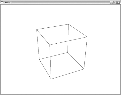
This line is much like the glDrawArrays function mentioned earlier, but now we are specifying an index array that determines the order in which the enabled vertex arrays are traversed. Figure 11.6 shows the output from the program CUBEDX.
Figure 11.6. A wireframe cube drawn with an indexed vertex array.
A variation on glDrawElement is the glDrawRangeElements function. This function is documented in Appendix C, “API Reference,” and simply adds two parameters to specify the range of indices that will be valid. This hint can enable some OpenGL implementations to prefetch the vertex data, a potentially worthwhile performance optimization. A further enhancement is glMultiDrawArrays, which allows you to send multiple arrays of indices with a single function call.
One last vertex array function you’ll find in the reference section is glInterleavedArrays. It allows you to combine several arrays into one aggregate array. There is no change to your access or traversal of the arrays, but the organization in memory can possibly enhance performance on some hardware implementations.
Getting Serious
With a few simple examples behind us, it’s time to tackle a more sophisticated model with more vertex data. For this example, we use a model of an F-16 Thunderbird created by Ed Womack at digitalmagician.net. We’ve used a commercial product called Deep Exploration (version 3.4) from Right Hemisphere that has a handy feature of exporting models as OpenGL code!
We had to modify the code output by Deep Exploration so that it would work with our GLUT framework and run on both the Macintosh and the PC platforms. You can find the code that renders the model in the THUNDERBIRD sample program. Note that the aircraft is broken up into two pieces: the main body and a much smaller glass canopy. For illustrational purposes, the following discussion will refer only to the larger body. We do not include the entire program listing here because it is quite lengthy and mostly meaningless to human beings. It consists of a number of arrays representing 3,704 individual triangles (that’s a lot of numbers to stare at!).
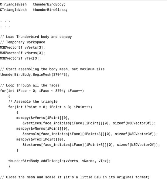
The approach taken with this tool is to try to produce the smallest possible amount of code to represent the given model. Deep Exploration has done a reasonable job of compacting the data. There are 3,704 individual triangles, but using a clever indexing scheme, Deep Exploration has encoded this as only 1,898 individual vertices, 2,716 normals, and 2,925 texture coordinates. The following code shows the DrawBody function, which loops through the index set and sends OpenGL the texture, normal, and vertex coordinates for each individual triangle:

This approach is okay when you must optimize the storage size of the model data—for example, to save memory in an embedded application, reduce storage space, or reduce bandwidth if the model must be transmitted over a network. However, for real-time applications in which performance considerations can sometimes outweigh memory constraints, this code would perform quite poorly because once again you are back to square one, sending vertex data to OpenGL one vertex at a time.
The simplest and perhaps most obvious approach to speeding up this code is simply to place the DrawModel function in a display list. Indeed, this is the approach we used in the THUNDERBIRD program that renders this model. You can see the output of the model in Figure 11.7.
Figure 11.7. An F-16 Thunderbird model.

Let’s look at the cost of this approach and compare it to rendering the same model with indexed vertex arrays. The Thunderbird model actually comes in two pieces: the main body and a transparent glass canopy. To keep things simple, we are neglecting the cost in these calculations of the separate and much smaller glass canopy.
Measuring the Cost
First, we calculate the amount of memory required to store the original compacted vertex data. We can do this simply by looking at the declarations of the data arrays and knowing how large the base data type is:
short face_indices[3704][9] = { ...
GLfloat vertices [1898][3] = { ...
GLfloat normals [2716][3] = { ...
GLfloat textures [2925][2] = { ...
The memory for face_indices would be sizeof(short) × 3,704 × 9, which works out to 66,672 bytes. Similarly, we calculate the size of vertices, normals, and textures as 22,776, 32,592, and 23,400 bytes, respectively. This gives us a total memory footprint of 145,440 bytes or about 142KB.
But wait! When we draw the model into the display list, we copy all this data again into the display list, except that now we decompress our packed data so that many vertices are duplicated for adjacent triangles. We, in essence, undo all the work to optimize the storage of the geometry to draw it. We can’t calculate exactly how much space the display list takes, but we can get a good estimate by calculating just the size of the geometry. There are 3,704 triangles. Each triangle has three vertices, each of which has a floating-point vertex (three floats), normal (three floats), and texture coordinate (two floats). Assuming 4 bytes for a float (sizeof(float)), we calculate this as shown here:
3,704 (triangle) × 3 (vertices) = 11,112 vertices
Each vertex has three components (x, y, z):
11,112 × 3 = 33,336 floating-point values for geometry
Each vertex has a normal, meaning three more components:
11,112 × 3 = 33,336 floating-point values for normals
Each vertex has a texture, meaning two more components:
11,112 × 2 = 22,224 floating-point values for texture coordinates
This gives a total of 88,896 floats, at 4 bytes each = 355,584 bytes.
Total memory for the display list data and the original data is then 501,024 bytes, just a tad shy of half a megabyte! But don’t forget the transformation cost—11,112 (3,704 × 3) vertices must be transformed by the OpenGL geometry pipeline. That’s a lot of matrix multiplies!
Creating a Suitable Indexed Array
Just because the data in the THUNDERBIRD sample is stored in arrays does not mean the data is ready to be used as any kind of OpenGL vertex array. In OpenGL, the vertex array, normal array, texture array, and any other arrays that you want to use must all be the same size. The reason is that all the array elements across arrays must be shared. For ordinary vertex arrays, as you march through the set of arrays, array element 0 from the vertex array must go with array element 0 from the normal array, and so on. For indexed arrays, we have the same requirement. Each index must address all the enabled arrays at the same corresponding array element.
For the sample program THUNDERGL, we have created a C++ utility class that processes the existing array data and reindexes the triangles so that all three arrays are the same size and all array elements correspond exactly one to another. Many 3D applications can benefit from reprocessing an unstructured list of triangles and creating a ready-to-go indexed vertex array. This class is easily reusable and extensible, and is placed in the shared source directory. Listing 11.3 shows the processing of the body and glass canopy elements to get the indexed array ready.
Listing 11.3. Code to Create the Indexed Vertex Arrays

First, we need to declare storage for our two new triangle meshes:
CTriangleMesh thunderBirdBody;
CTriangleMesh thunderBirdGlass;
Then in the SetupRC function, we populate these triangle meshes with triangles. Because we don’t know ahead of time what our savings will be, when we start the mesh, we must tell the class the maximum amount of storage to allocate for workspace. We know that the face array (each containing three vertices) is 3,704 elements long, so the worst possible scenario is 3,704 × 3 unique vertices. As we will see, we will actually do much better than this.
thunderBirdBody.BeginMesh(3704*3);
Finally, we loop through all the faces, assemble each triangle individually, and send it the AddTriangle method. When all the triangles are added, we scale them using the member function Scale. We did this only because the original model data was bigger than we’d prefer.
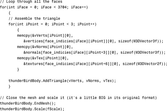
We must do this for both the Thunderbird body and the glass canopy.
Comparing the Cost
Now let’s compare the cost of our three methods of rendering this model. The CTriangleMesh class reports that the processed body of the Thunderbird consists of 3,265 unique vertices (including matching normals and texture coordinates), and 11,112 indexes (which is the total number of vertices when rendered as triangles). Each vertex and normal has three components (x,y,z), and each texture coordinate has two components. The total number of floating-point values in the mesh data is then calculated this way:
3,265 vertices × 8 = 26,120 floats
Multiplying each float by 4 bytes yields a memory overhead of 104,480 bytes. We still need to add in the index array of unsigned shorts. That’s another 11,112 elements times 2 bytes each = 22,224. This gives a grand total storage overhead of 126,704 bytes. Table 11.2 shows these values side by side. Remember, a kilobyte is 1,024 bytes.
Table 11.2. Memory and Transformation Overhead for Three Rendering Methods

As it turns out in this case, the Indexed Vertex Array approach wins hands down in terms of memory footprint, and requires less than one-third of the transformation work on the vertices!
In a production program, you might have tools that take this calculated indexed array and write it out to disk with a header that describes the required array dimensions. Reading this mesh or a collection of meshes back into the program then is a simple implementation of a basic model loader. The loaded model’s meshes are then exactly in the format required by OpenGL.
Models with sharp edges and corners often have fewer vertices that are candidates for sharing. However, models with large smooth surface areas can stand to gain even more in terms of memory and transformation savings. With the added savings of less geometry to move through memory, and the corresponding savings in matrix operations, indexed vertex arrays can sometimes outperform display lists. For many real-time applications, indexed vertex arrays are often the method of choice for geometric rendering. As you’ll soon see, we can take still one more step forward with our vertex arrays and achieve the fastest possible performance, leaving even display lists in the dust!
Back to the point
With all this multiplication and addition going on, we almost forgot that we were trying to render something! The THUNDERGL sample program is a good opportunity to showcase all we have learned so far in this book. Rather than simply render the model against a blank background, we are going to adapt this model to Chapter 9’s CUBEMAP sample program. In addition to a nice skybox for the background, we will make use of cube mapping and multitexture to make the glass canopy really look like a glass canopy.
As in the CUBEMAP sample program, we begin by rendering the skybox using the cube map texture. To render the Thunderbird body, we call the function shown in Listing 11.4.
Listing 11.4. Code to the Entire Thunderbird Model

The model this time is rendered as an indexed vertex array. Just like non-indexed arrays, we must enable the vertex arrays we want to use:
glEnableClientState(GL_VERTEX_ARRAY);
glEnableClientState(GL_NORMAL_ARRAY);
glEnableClientState(GL_TEXTURE_COORD_ARRAY);
To render the body, we turn off the cube map that is bound to the second texture unit, and just draw the body, using a modulated texture environment so that the shading of the geometry shows through the texture. We will need to do a small rotation to orient the model the way we want it presented:
glActiveTexture(GL_TEXTURE1);
glDisable(GL_TEXTURE_CUBE_MAP);
glActiveTexture(GL_TEXTURE0);
glPushMatrix();
glRotatef(-90.0f, 1.0f, 0.0f, 0.0f);
glTexEnvi(GL_TEXTURE_2D, GL_TEXTURE_ENV_MODE, GL_MODULATE);
glBindTexture(GL_TEXTURE_2D, textureObjects[BODY_TEXTURE]);
thunderBirdBody.Draw();
glPopMatrix();
The Draw method of the CTriangleMesh class instance thunderBirdBody simply sets the vertex pointers, and calls glDrawElements.
// Draw - make sure you call glEnableClientState for these arrays
void CTriangleMesh::Draw(void) {
// Here's where the data is now
glVertexPointer(3, GL_FLOAT,0, pVerts);
glNormalPointer(GL_FLOAT, 0, pNorms);
glTexCoordPointer(2, GL_FLOAT, 0, pTexCoords);
// Draw them
glDrawElements(GL_TRIANGLES, nNumIndexes, GL_UNSIGNED_INT, pIndexes);
}
The glass canopy is a real showcase item here. First we turn cube mapping back on, but on the second texture unit. We have also previously (not shown here) enabled a reflective texture coordinate generation mode for the cube map on this texture unit.
glActiveTexture(GL_TEXTURE1);
glEnable(GL_TEXTURE_CUBE_MAP);
glActiveTexture(GL_TEXTURE0);
To draw the canopy transparently, we turn on blending and use the standard transparency blending mode. The alpha value for the material is turned way down to make the glass mostly clear:
glEnable(GL_BLEND);
glBlendFunc(GL_SRC_ALPHA, GL_ONE_MINUS_SRC_ALPHA);
glColor4f(1.0f, 1.0f, 1.0f, 0.25f);
glBindTexture(GL_TEXTURE_2D, textureObjects[GLASS_TEXTURE]);
Then we make a minor position tweak to the canopy and draw it twice:
glTranslatef(0.0f, 0.132f, 0.555f);
glFrontFace(GL_CW);
thunderBirdGlass.Draw();
glFrontFace(GL_CCW);
thunderBirdGlass.Draw();
glDisable(GL_BLEND);
Why did we draw the canopy twice? If you recall from Chapter 6, “More on Colors and Materials,” the trick to transparency is to draw the background object first. This is the reason we rendered the plane body first, and the canopy second. Regardless of orientation, the canopy either will be hidden via the depth test behind the plane body, or will be drawn second but in front of the body. But the canopy itself has an inside and an outside visible when you look through it from the outside. The simple trick here is to flip front-facing polygons to GL_CW temporarily and draw the object. This draws the back side of the object first, which is also the part of the object farthest away. Restoring front-facing polygons to GL_CCW and drawing the object again draws just the front side of the object, neatly on top of the just-rendered back side. With blending on during this entire operation, you get a nice transparent piece of glass. With the cube map added in as well, you get a very believable glassy reflective surface. The result is shown in Figure 11.8, and in Color Plate 6. Neither image, however, matches the effect of seeing the animation onscreen.
Figure 11.8. The final Thunderbird model. (This figure also appears in the Color insert.)

Vertex Buffer Objects
Display lists are a quick and easy way to optimize immediate mode code (code using glBegin/glEnd). At the very worst, a display list will contain a precompiled set of OpenGL data, ready to be copied quickly to the command buffer, and destined for the graphics hardware. At best, an implementation may copy a display list to the graphics hardware, reducing bandwidth to the hardware to essentially nil. This last scenario is highly desirable, but is a bit of a luck-of-the-draw performance optimization. Display lists are also not terribly flexible after they are created!
Vertex arrays, on the other hand, give us all the flexibility we want, and at worst result in block copies (still much faster than immediate mode) to the hardware. Indexed vertex arrays further up the ante by providing a means of reducing the amount of vertex data that must be transferred to the hardware, and reducing the transformation overhead. For dynamic geometry such as cloth, water, or just trees swaying in the wind, vertex arrays are an obvious choice.
There is one more feature of OpenGL that provides the ultimate control over geometric throughput. When you’re using vertex arrays, it is possible to transfer individual arrays from your client (CPU-accessible) memory to the graphics hardware. This feature, vertex buffer objects, allow you to use and manage vertex array data in a similar manner to how we load and manage textures. Vertex buffer objects, however, are far more flexible than texture objects.
Managing and Using Buffer Objects
The first step to using vertex buffer objects is to use vertex arrays. We have that well covered at this point. The second step is to create the buffer objects in a manner similar to creating texture objects. To do this, we use the function glGenBuffers:
void glGenBuffers(GLsizei n, GLuint *buffers);
This function works just like the glGenTextures function covered in Chapter 8, “Texture Mapping: The Basics.” The first parameter is the number of buffer objects desired, and the second is an array that is filled with new vertex buffer object names. In an identical way, buffers are released with glDeleteBuffers.
Vertex buffer objects are “bound,” again reminding us of the use of texture objects. The function glBindBuffer binds the current state to a particular buffer object:
void glBindBuffer(GLenum target, GLuint buffer);
Here, target refers to the kind of array being bound (again, similar to texture targets). This may be either GL_ARRAY_BUFFER for vertex data (including normals, texture coordinates, etc.) or GL_ELEMENT_ARRAY_BUFFER for array indexes to be used with glDrawElements and the other index-based rendering functions.
Loading the Buffer Objects
To copy your vertex data to the graphics hardware, you first bind to the buffer object in question, then call glBufferData:
void glBufferData(GLenum target, GLsizeiptr size, GLvoid *data, GLenum usage);
Again target refers to either GL_ARRAY_BUFFER or GL_ELEMENT_ARRAY_BUFFER, and size refers to the size in bytes of the vertex array. The final parameter is a performance usage hint. This can be any one of the values listed in Table 11.3.
Table 11.3. Buffer Object Usage Hints

Rendering from VBOs
Two things change when rendering from vertex array objects. First, you must bind to the specific vertex array before calling one of the vertex pointer functions. Second, the actual pointer to the array now becomes an offset into the vertex buffer object. For example,
glVertexPointer(3, GL_FLOAT,0, pVerts);
now becomes this:
glBindBuffer(GL_ARRAY_BUFFER, bufferObjects[0]);
glVertexPointer(3, GL_FLOAT,0, 0);
This goes for the rendering call as well; for example:
glBindBuffer(GL_ELEMENT_ARRAY_BUFFER, bufferObjects[3]);
glDrawElements(GL_TRIANGLES, nNumIndexes, GL_UNSIGNED_SHORT, 0);
This offset into the buffer object is technically an offset based on the native architecture’s NULL pointer. On most systems, this is just zero.
Back to the Thunderbird!
Let’s apply what we have learned to our Thunderbird model so that we can see all of this in a real context. The sample program VBO from this chapter’s sample source code is adapted from the THUNDERGL sample program, but it has been retrofitted to use vertex buffer objects. The only change to the main program’s source code is that the CTriangleMesh objects have been replaced with CVBOMesh objects. The CVBOMesh class is nothing more than the CTriangleMesh class revved up to use VBOs. Two small changes were made to the header. We defined four values to represent each of our four arrays:
#define VERTEX_DATA 0
#define NORMAL_DATA 1
#define TEXTURE_DATA 2
#define INDEX_DATA 3
And we need storage for the four buffer objects:
GLuint bufferObjects[4];
Initializing the Arrays
The biggest change to the original code is in the EndMesh method, shown in Listing 11.5.
Listing 11.5. The New End Mesh Method


As outlined in the previous section, each array is loaded individually into its own buffer object. Notice that after the data is copied to the buffer object, the original pointer is no longer needed, and all the working space buffers are deleted. This has three implications. First, it frees up client memory, which you can never have enough of. Second, it consumes memory on the graphics hardware, which you never seem to have enough of! Third, you can no longer make changes to the data, because you no longer have access to it. What about dynamic geometry?
Mixing static and dynamic data
There are two methods of handling dynamic or regularly changing geometry. The first is to simply not use VBOs for the arrays that are being regularly updated. For example, if you have a cloth animation, the texture coordinates on your mesh are unlikely to change frame to frame, whereas the vertices are constantly being updated. You can put the texture coordinates in a VBO, and keep the vertex data in a regular vertex array. After you call glBindBuffer, though, you are bound to a particular VBO. Calling glBindBuffer again switches to another VBO. How then do we “unbind” and go back to regular vertex arrays? Simple, just bind to a NULL buffer:
glBindBuffer(GL_ARRAY_BUFFER, 0);
If the data doesn’t need to be updated all that often, another alternative is to map the buffer back into client memory. This actually comes up in the CVBOMesh class Scale function as shown here:
glBindBuffer(GL_ARRAY_BUFFER, bufferObjects[VERTEX_DATA]);
M3DVector3f *pVertexData = (M3DVector3f *)glMapBuffer(GL_ARRAY_BUFFER,
GL_READ_WRITE);
if(pVertexData != NULL)
{
for(int i = 0; i < nNumVerts; i++)
m3dScaleVector3(pVertexData[i], fScaleValue);
glUnmapBuffer(GL_ARRAY_BUFFER);
}
The glMapBuffer function returns a pointer that you can use to access the vertex data directly. The second parameter to this function is the access permissions and may be GL_READ_WRITE, GL_WRITE_ONLY, or GL_READ_ONLY. When you do this, you must unmap the buffer with glUnmapBuffer before you can use the buffer object again.
Render!
Finally, we are ready to render our model using vertex buffer objects. Listing 11.6 shows the new and improved Draw method. Now, when you run the sample program VBO (which looks just like THUNDERGL!), both the textures and all the geometry are being rendered on the graphics card from local memory. This is the best possible scenario, because the bandwidth to the hardware is virtually nonexistent compared to using vertex arrays, or using worst-case optimized display lists.
Listing 11.6. The New and Improved Draw Method

Summary
In this chapter, we focused on different methods of improving geometric throughput. We began with display lists, which are an excellent way to quickly optimize legacy immediate mode rendering code. Display lists, however, can also be used conveniently to store many other OpenGL commands such as state changes, lighting setup, and any other frequently repeated tasks.
By packing all the vertex data together in a single data structure (an array), you enable the OpenGL implementation to make potentially valuable performance optimizations. In addition, you can stream the data to disk and back, thus storing the geometry in a format that is ready for use in OpenGL. Although OpenGL does not have a “model format” as some higher level APIs do, the vertex array construct is certainly a good place to start if you want to build your own.
Generally, you can significantly speed up static geometry by using display lists, and you can use vertex arrays whenever you want dynamic geometry. Index vertex arrays, on the other hand, can potentially (but not always) give you the best of both worlds—flexible geometry data and highly efficient memory transfer and geometric processing. For many applications, vertex arrays are used almost exclusively. However, the old glBegin/glEnd construct still has many uses, besides allowing you to create display lists—anytime the amount of geometry fluctuates dynamically from frame to frame, for example. There is little benefit to continually rebuilding a small vertex array from scratch rather than letting the driver do the work with glBegin/glEnd.
Finally, we learned to use vertex buffer objects to get the best possible optimization we can hope for with display lists (storing the geometry on the hardware) yet have the great flexibility of using vertex arrays. We’ve seen that the best possible way to render static geometry is to represent it as an indexed vertex array, and store it on your graphics card via VBOs. Still, we have only scratched the surface of OpenGL’s rich buffer object feature set. In Chapter 18, “Advanced Buffers,” you’ll learn some more powerful optimizations and whole new capabilities made possible by the ideas introduced in this chapter.