
Chapter 9. Texture Mapping: Beyond the Basics
WHAT YOU’LL LEARN IN THIS CHAPTER:

Texture mapping is perhaps one of the most exciting features of OpenGL (well, close behind shaders anyway!) and is heavily relied on in the games and simulation industry. In Chapter 8, “Texture Mapping: The Basics,” you learned the basics of loading and applying texture maps to geometry. In this chapter, we’ll expand on this knowledge and cover some of the finer points of texture mapping in OpenGL.
Secondary Color
Applying texture to geometry, in regard to how lighting works, causes a hidden and often undesirable side effect. In general, you set the texture environment to GL_MODULATE, causing lit geometry to be combined with the texture map in such a way that the textured geometry also appears lit. Normally, OpenGL performs lighting calculations and calculates the color of individual fragments according to the standard light model. These fragment colors are then multiplied by the filtered texel colors being applied to the geometry. However, this process has the side effect of suppressing the visibility of specular highlights on the geometry. Basically, any texture color multiplied by ones (the white spot) is the same texture color. You cannot, by multiplication of any number less than or equal to one, make a color brighter than it already is!
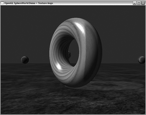
For example, Figure 9.1 shows the original lit SPHEREWORLD sample from Chapter 5, “Color, Materials, and Lighting: The Basics.” In this figure, you can see clearly the specular highlights reflecting off the surface of the torus. In contrast, Figure 9.2 shows the SPHEREWORLD sample from Chapter 8. In this figure, you can see the effects of having the texture applied after the lighting has been added.
Figure 9.1. The original SPHEREWORLD torus with specular highlights.

Figure 9.2. The textured torus with muted highlights.

The solution to this problem is to apply (by adding instead of multiplication) the specular highlights after texturing. This technique, called the secondary specular color, can be manually applied or automatically calculated by the lighting model. Usually, you do this using the normal OpenGL lighting model and simply turn it on using glLightModeli, as shown here:
glLightModeli(GL_LIGHT_MODEL_COLOR_CONTROL, GL_SEPARATE_SPECULAR_COLOR);
You can switch back to the normal lighting model by specifying GL_SINGLE_COLOR for the light model parameter:
glLightModeli(GL_LIGHT_MODEL_COLOR_CONTROL, GL_COLOR_SINGLE);
Figure 9.3 shows the output from this chapter’s version of SPHEREWORLD with the restored specular highlights on the torus. We do not provide a listing for this sample because it simply contains the addition of the preceding single line of code.
Figure 9.3. Highlights restored to the textured torus.
You can also directly specify a secondary color after texturing when you are not using lighting (lighting is disabled) using the glSecondaryColor function. This function comes in many variations just as glColor does and is fully documented in the reference section. You should also note that if you specify a secondary color, you must also explicitly enable the use of the secondary color by enabling the GL_COLOR_SUM flag:
glEnable(GL_COLOR_SUM);
Manually setting the secondary color only works when lighting is disabled.
Anisotropic Filtering
Anisotropic texture filtering is not a part of the core OpenGL specification, but it is a widely supported extension that can dramatically improve the quality of texture filtering operations. Texture filtering is covered in the preceding chapter, where you learned about the two basic texture filters: nearest neighbor (GL_NEAREST) and linear (GL_LINEAR). When a texture map is filtered, OpenGL uses the texture coordinates to figure out where in the texture map a particular fragment of geometry falls. The texels immediately around that position are then sampled using either the GL_NEAREST or the GL_LINEAR filtering operations.
This process works perfectly when the geometry being textured is viewed directly perpendicular to the viewpoint, as shown on the left in Figure 9.4. However, when the geometry is viewed from an angle more oblique to the point of view, a regular sampling of the surrounding texels results in the loss of some information in the texture (it looks blurry!). A more realistic and accurate sample would be elongated along the direction of the plane containing the texture. This result is shown on the right in Figure 9.4. Taking this viewing angle into account for texture filtering is called anisotropic filtering.
Figure 9.4. Normal texture sampling versus anisotropic sampling.

You can apply anisotropic filtering to any of the basic or mipmapped texture filtering modes; applying it requires three steps. First, you must determine whether the extension is supported. You can do this by querying for the extension string GL_EXT_texture_filter_anisotropic. You can use the glTools function named gltIsExtSupported for this task:
if(gltIsExtSupported("GL_EXT_texture_filter_anisotropic"))
// Set Flag that extension is supported
After you determine that this extension is supported, you can find the maximum amount of anisotropy supported. You can query for it using glGetFloatv and the parameter GL_MAX_TEXTURE_MAX_ANISOTROPY_EXT:
GLfloat fLargest;
. . .
. . .
glGetFloatv(GL_MAX_TEXTURE_MAX_ANISOTROPY_EXT, &fLargest);
The larger the amount of anisotropy applied, the more texels are sampled along the direction of greatest change (along the strongest point of view). A value of 1.0 represents normal texture filtering (called isotropic filtering). Bear in mind that anisotropic filtering is not free. The extra amount of work, including other texels, can sometimes result in substantial performance penalties. On modern hardware, this feature is getting quite fast and is becoming a standard feature of popular games, animation, and simulation programs.
Finally, you set the amount of anisotropy you want applied using glTexParameter and the constant GL_TEXTURE_MAX_ANISOTROPY_EXT. For example, using the preceding code, if you want the maximum amount of anisotropy applied, you would call glTexParameterf as shown here:
glTexParameterf(GL_TEXTURE_2D, GL_TEXTURE_MAX_ANISOTROPY_EXT, fLargest);
This modifier is applied per texture object just like the standard filtering parameters.
The sample program ANISOTROPIC provides a striking example of anisotropic texture filtering in action. This program displays a tunnel with walls, a floor, and ceiling geometry. The arrow keys move your point of view (or the tunnel) back and forth along the tunnel interior. A right mouse click brings up a menu that allows you to select from the various texture filters, and turn on and off anisotropic filtering. Figure 9.5 shows the tunnel using trilinear filtered mipmapping. Notice how blurred the patterns become in the distance, particularly with the bricks.
Figure 9.5. ANISOTROPIC tunnel sample with trilinear filtering.

Now compare Figure 9.5 with Figure 9.6, in which anisotropic filtering has been enabled. The mortar between the bricks is now clearly visible all the way to the end of the tunnel. In fact, anisotropic filtering can also greatly reduce the visible mipmap transition patterns for the GL_LINEAR_MIPMAP_NEAREST and GL_NEAREST_MIPMAP_NEAREST mipmapped filters.
Figure 9.6. ANISOTROPIC tunnel sample with anisotropic filtering.

Texture Compression
Texture mapping can add incredible realism to any 3D rendered scene, with a minimal cost in vertex processing. One drawback to using textures, however, is that they require a lot of memory to store and process. Early attempts at texture compression were crudely storing textures as JPG files and decompressing the textures when loaded before calling glTexImage. These attempts saved disk space or reduced the amount of time required to transmit the image over the network (such as the Internet), but did nothing to alleviate the storage requirements of texture images loaded into graphics hardware memory.
Native support for texture compression was added to OpenGL with version 1.3. Earlier versions of OpenGL may also support texture compression via extension functions of the same name. You can test for this extension by using the GL_ARB_texture_compression string.
Texture compression support in OpenGL hardware can go beyond simply allowing you to load a compressed texture; in most implementations, the texture data stays compressed even in the graphics hardware memory. This allows you to load more texture into less memory and can significantly improve texturing performance due to fewer texture swaps (moving textures around) and fewer memory accesses during texture filtering.
Compressing Textures
Texture data does not have to be initially compressed to take advantage of OpenGL support for compressed textures. You can request that OpenGL compress a texture image when loaded by using one of the values in Table 9.1 for the internalFormat parameter of any of the glTexImage functions.
Table 9.1. Compressed Texture Formats

Compressing images this way adds a bit of overhead to texture loads but can increase texture performance due to the more efficient usage of texture memory. If, for some reason, the texture cannot be compressed, OpenGL uses the base internal format listed instead and loads the texture uncompressed.
When you attempt to load and compress a texture in this way, you can find out whether the texture was successfully compressed by using glGetTexLevelParameteriv with GL_TEXTURE_COMPRESSED as the parameter name:
GLint compFlag;
. . .
glGetTexLevelParameteriv(GL_TEXTURE_2D, 0, GL_TEXTURE_COMPRESSED, &compFlag);
The glGetTexLevelParameteriv function accepts a number of new parameter names pertaining to compressed textures. These parameters are listed in Table 9.2.
Table 9.2. Compressed Texture Parameters Retrieved with glGetTexLevelParameter

When textures are compressed using the values listed in Table 9.1, OpenGL chooses the most appropriate texture compression format. You can use glHint to specify whether you want OpenGL to choose based on the fastest or highest quality algorithm:
glHint(GL_TEXTURE_COMPRESSION_HINT, GL_FASTEST);
glHint(GL_TEXTURE_COMPRESSION_HINT, GL_NICEST);
glHint(GL_TEXTURE_COMPRESSION_HINT, GL_DONT_CARE);
The exact compression format varies from implementation to implementation. You can obtain a count of compression formats and a list of the values by using GL_NUM_COMPRESSED_TEXTURE_FORMATS and GL_COMPRESSED_TEXTURE_FORMATS. To check for support for a specific set of compressed texture formats, you need to check for a specific extension for those formats. For example, nearly all implementations support the GL_EXT_texture_compression_s3tc texture compression format. If this extension is supported, the compressed texture formats listed in Table 9.3 are all supported, but only for two-dimensional textures.
Table 9.3. Compression Formats for GL_EXT_texture_compression_s3tc

Loading Compressed Textures
Using the functions in the preceding section, you can have OpenGL compress textures in a natively supported format, retrieve the compressed data with the glGetCompressedTexImage function (identical to the glGetTexImage function for uncompressed textures), and save it to disk. On subsequent loads, the raw compressed data can be used, resulting in substantially faster texture loads. Be advised, however, that some vendors may cheat a little when it comes to texture loading in order to optimize texture storage or filtering operations. This technique will work only on fully conformant hardware implementations.
To load precompressed texture data, use one of the following functions:
void glCompressedTexImage1D(GLenum target, GLint level, GLenum internalFormat,
GLsizei width,
GLint border, GLsizei imageSize, void *data);
void glCompressedTexImage2D(GLenum target, GLint level, GLenum internalFormat,
GLsizei width, GLsizei height,
GLint border, GLsizei imageSize, void *data);
void glCompressedTexImage3D(GLenum target, GLint level, GLenum internalFormat,
GLsizei width, GLsizei height, GLsizei depth,
GLint border, Glsizei imageSize, GLvoid *data);
These functions are virtually identical to the glTexImage functions from the preceding chapter. The only difference is that the internalFormat parameter must specify a supported compressed texture image. If the implementation supports the GL_EXT_texture_compression_s3tc extension, this would be one of the values from Table 9.3. There is also a corresponding set of glCompressedTexSubImage functions for updating a portion or all of an already-loaded texture that mirrors the glTexSubImage functionality from the preceding chapter.
Texture compression is a very popular texture feature. Smaller textures take up less storage, transmit faster over networks, load faster off disk, copy faster to graphics memory, allow for substantially more texture to be loaded onto hardware, and generally texture slightly faster to boot! Don’t forget, though, as with so many things in life, there is no such thing as a free lunch. Something may be lost in the compression. The GL_EXT_texture_compression_s3tc method, for example, works by stripping color data out of each texel. For some textures, this results in substantial image quality loss (particularly for textures that contain smooth color gradients). Other times, textures with a great deal of detail are visually nearly identical to the original uncompressed version. The choice of texture compression method (or indeed no compression) can vary greatly depending on the nature of the underlying image.
Texture Coordinate Generation
In Chapter 8, you learned that textures are mapped to geometry using texture coordinates. Often, when you are loading models (see Chapter 11, “It’s All About the Pipeline: Faster Geometry Throughput”), texture coordinates are provided for you. If necessary, you can easily map texture coordinates manually to some surfaces such as spheres or flat planes. Sometimes, however, you may have a complex surface for which it is not so easy to manually derive the coordinates. OpenGL can automatically generate texture coordinates for you within certain limitations.
Texture coordinate generation is enabled on the S, T, R, and Q texture coordinates using glEnable:
glEnable(GL_TEXTURE_GEN_S);
glEnable(GL_TEXTURE_GEN_T);
glEnable(GL_TEXTURE_GEN_R);
glEnable(GL_TEXTURE_GEN_Q);
When texture coordinate generation is enabled, any calls to glTexCoord are ignored, and OpenGL calculates the texture coordinates for each vertex for you. In the same manner that texture coordinate generation is turned on, you turn it off by using glDisable:
glDisable(GL_TEXTURE_GEN_S);
glDisable(GL_TEXTURE_GEN_T);
glDisable(GL_TEXTURE_GEN_R);
glDisable(GL_TEXTURE_GEN_Q);
You set the function or method used to generate texture coordinates with the following functions:
void glTexGenf(GLenum coord, GLenum pname, GLfloat param);
void glTexGenfv(GLenum coord, GLenum pname, GLfloat *param);
The first parameter, coord, specifies which texture coordinate this function sets. It must be GL_S, GL_T, GL_R, or GL_Q. The second parameter, pname, must be GL_TEXTURE_GEN_MODE, GL_OBJECT_PLANE, or GL_EYE_PLANE. The last parameter sets the values of the texture generation function or mode. Note that integer (GLint) and double (GLdouble) versions of these functions are also used.
The pertinent portions of the sample program TEXGEN are presented in Listing 9.1. This program displays a torus that can be manipulated (rotated around) using the arrow keys. A right-click brings up a context menu that allows you to select from the first three texture generation modes we will discuss: Object Linear, Eye Linear, and Sphere Mapping.
Listing 9.1. Source Code for the TEXGEN Sample Program


Object Linear Mapping
When the texture generation mode is set to GL_OBJECT_LINEAR, texture coordinates are generated using the following function:
coord = P1*X + P2*Y + P3*Z + P4*W
The X, Y, Z, and W values are the vertex coordinates from the object being textured, and the P1–P4 values are the coefficients for a plane equation. The texture coordinates are then projected onto the geometry from the perspective of this plane. For example, to project texture coordinates for S and T from the plane Z = 0, we would use the following code from the TEXGEN sample program:
// Projection plane
GLfloat zPlane[] = { 0.0f, 0.0f, 1.0f, 0.0f };
. . .
. . .
// Object Linear
glTexGeni(GL_S, GL_TEXTURE_GEN_MODE, GL_OBJECT_LINEAR);
glTexGeni(GL_T, GL_TEXTURE_GEN_MODE, GL_OBJECT_LINEAR);
glTexGenfv(GL_S, GL_OBJECT_PLANE, zPlane);
glTexGenfv(GL_T, GL_OBJECT_PLANE, zPlane);
Note that the texture coordinate generation function can be based on a different plane equation for each coordinate. Here, we simply use the same one for both the S and the T coordinates.
This technique maps the texture to the object in object coordinates, regardless of any modelview transformation in effect. Figure 9.7 shows the output for TEXGEN when the Object Linear mode is selected. No matter how you reorient the torus, the mapping remains fixed to the geometry.
Figure 9.7. Torus mapped with object linear coordinates.

Eye Linear Mapping
When the texture generation mode is set to GL_EYE_LINEAR, texture coordinates are generated in a similar manner to GL_OBJECT_LINEAR. The coordinate generation looks the same, except that now the X, Y, Z, and W coordinates indicate the location of the point of view (where the camera or eye is located). The plane equation coefficients are also inverted before being applied to the equation to account for the fact that now everything is in eye coordinates.
The texture, therefore, is basically projected from the plane onto the geometry. As the geometry is transformed by the modelview matrix, the texture will appear to slide across the surface. We set up this capability with the following code from the TEXGEN sample program:
// Projection plane
GLfloat zPlane[] = { 0.0f, 0.0f, 1.0f, 0.0f };
. . .
. . .
// Eye Linear
glTexGeni(GL_S, GL_TEXTURE_GEN_MODE, GL_EYE_LINEAR);
glTexGeni(GL_T, GL_TEXTURE_GEN_MODE, GL_EYE_LINEAR);
glTexGenfv(GL_S, GL_EYE_PLANE, zPlane);
glTexGenfv(GL_T, GL_EYE_PLANE, zPlane);
The output of the TEXGEN program when the Eye Linear menu option is selected is shown in Figure 9.8. As you move the torus around with the arrow keys, note how the projected texture slides about on the geometry.
Figure 9.8. An example of eye linear texture mapping.

Sphere Mapping
When the texture generation mode is set to GL_SPHERE_MAP, OpenGL calculates texture coordinates in such a way that the object appears to be reflecting the current texture map. This is the easiest mode to set up, with just these two lines from the TEXGEN sample program:
glTexGeni(GL_S, GL_TEXTURE_GEN_MODE, GL_SPHERE_MAP);
glTexGeni(GL_T, GL_TEXTURE_GEN_MODE, GL_SPHERE_MAP);
You usually can make a well-constructed texture by taking a photograph through a fish-eye lens. This texture then lends a convincing reflective quality to the geometry. For more realistic results, sphere mapping has largely been replaced by cube mapping (discussed next). However, sphere mapping still has some uses because it has significantly less overhead.
In particular, sphere mapping requires only a single texture instead of six, and if true reflectivity is not required, you can obtain adequate results from sphere mapping. Even without a well-formed texture taken through a fish-eye lens, you can also use sphere mapping for an approximate environment map. Many surfaces are shiny and reflect the light from their surroundings, but are not mirror-like in their reflective qualities. In the TEXGEN sample program, we use a suitable environment map for the background (all modes show this background), as well as the source for the sphere map. Figure 9.9 shows the environment-mapped torus against a similarly colored background. Moving the torus around with the arrow keys produces a reasonable approximation of a reflective surface.
Figure 9.9. An environment map using a sphere map.

Cube Mapping
The last two texture generation modes, GL_REFLECTION_MAP and GL_NORMAL_MAP, require the use of a new type of texture target: the cube map. A cube map is treated as a single texture, but is made up of six square (yes, they must be square!) 2D images that make up the six sides of a cube. Figure 9.10 shows the layout of six square textures composing a cube map for the CUBEMAP sample program.
Figure 9.10. The layout of six cube faces in the CUBEMAP sample program.

These six 2D tiles represent the view of the world from six different directions (negative and positive X, Y, and Z). Using the texture generation mode GL_REFLECTION_MAP, you can then create a realistically reflective surface.
Loading Cube Maps
Cube maps add six new values that can be passed into glTexImage2D: GL_TEXTURE_CUBE_MAP_POSITIVE_X, GL_TEXTURE_CUBE_MAP_NEGATIVE_X, GL_TEXTURE_CUBE_MAP_POSITIVE_Y, GL_TEXTURE_CUBE_MAP_NEGATIVE_Y, GL_TEXTURE_CUBE_MAP_POSITIVE_Z, and GL_TEXTURE_CUBE_MAP_NEGATIVE_Z. These constants represent the direction in world coordinates of the cube face surrounding the object being mapped. For example, to load the map for the positive X direction, you might use a function that looks like this:
glTexImage2D(GL_TEXTURE_CUBE_MAP_POSITIVE_X, 0, GL_RGBA, iWidth, iHeight,
0, GL_RGBA, GL_UNSIGNED_BYTE, pImage);
To take this example further, look at the following code segment from the CUBEMAP sample program. Here, we store the name and identifiers of the six cube maps in arrays and then use a loop to load all six images into a single texture object:

To enable the application of the cube map, we now call glEnable with GL_TEXTURE_CUBE_MAP instead of GL_TEXTURE_2D (we also use the same value in glBindTexture when using texture objects):
glEnable(GL_TEXTURE_CUBE_MAP);
If both GL_TEXTURE_CUBE_MAP and GL_TEXTURE_2D are enabled, GL_TEXTURE_CUBE_MAP has precedence. Also, notice that the texture parameter values (set with glTexParameter) affect all six images in a single cube texture.
Texture coordinates for cube maps seem a little odd at first glance. Unlike a true 3D texture, the S, T, and R texture coordinates represent a signed vector from the center of the texture map. This vector intersects one of the six sides of the cube map. The texels around this intersection point are then sampled to create the filtered color value from the texture.
Using Cube Maps
The most common use of cube maps is to create an object that reflects its surroundings. The six images used for the CUBEMAP sample program were provided courtesy of The Game Creators, Ltd. (www.thegamecreators.com). This cube map is applied to a sphere, creating the appearance of a mirrored surface. This same cube map is also applied to the skybox, which creates the background being reflected.
A skybox is nothing more than a big box with a picture of the sky on it. Another way of looking at it is as a picture of the sky on a big box! Simple enough. An effective skybox contains six images that contain views from the center of your scene along the six directional axes. If this sounds just like a cube map, congratulations, you’re paying attention! For our CUBEMAP sample program a large box is drawn around the scene, and the CUBEMAP texture is applied to the six faces of the cube. The skybox is drawn as a single batch of six GL_QUADS. Each face is then manually textured using glTexCoord3f. For each vertex, a vector is specified that points to that corner of the sky box. The first side (in the negative X direction) is shown here:
glBegin(GL_QUADS);
//////////////////////////////////////////////
// Negative X
glTexCoord3f(-1.0f, -1.0f, 1.0f);
glVertex3f(-fExtent, -fExtent, fExtent);
glTexCoord3f(-1.0f, -1.0f, -1.0f);
glVertex3f(-fExtent, -fExtent, -fExtent);
glTexCoord3f(-1.0f, 1.0f, -1.0f);
glVertex3f(-fExtent, fExtent, -fExtent);
glTexCoord3f(-1.0f, 1.0f, 1.0f);
glVertex3f(-fExtent, fExtent, fExtent);
. . .
. . .
It is important to remember that in order for the manual selection of texture coordinates via glTexCoord3f to work, you must disable the texture coordinate generation:
// Sky Box is manually textured
glDisable(GL_TEXTURE_GEN_S);
glDisable(GL_TEXTURE_GEN_T);
glDisable(GL_TEXTURE_GEN_R);
DrawSkyBox();
To draw the reflective sphere, the CUBEMAP sample sets the texture generation mode to GL_REFLECTION_MAP for all three texture coordinates:
glTexGeni(GL_S, GL_TEXTURE_GEN_MODE, GL_REFLECTION_MAP);
glTexGeni(GL_T, GL_TEXTURE_GEN_MODE, GL_REFLECTION_MAP);
glTexGeni(GL_R, GL_TEXTURE_GEN_MODE, GL_REFLECTION_MAP);
We must also make sure that texture coordinate generation is enabled:
// Use texgen to apply cube map
glEnable(GL_TEXTURE_GEN_S);
glEnable(GL_TEXTURE_GEN_T);
glEnable(GL_TEXTURE_GEN_R);
To provide a true reflection, we also take the orientation of the camera into account. The camera’s rotation matrix is extracted from the camera class, and inverted. This is then applied to the texture matrix before the cube map is applied. Without this rotation of the texture coordinates, the cube map will not correctly reflect the surrounding skybox. Since the gltDrawSphere function makes no modelview matrix mode changes, we can also leave the matrix mode as GL_TEXTURE until we are through drawing and have restored the texture matrix to its original state (usually this will be the identity matrix):
glMatrixMode(GL_TEXTURE);
glPushMatrix();
// Invert camera matrix (rotation only) and apply to
// texture coordinates
M3DMatrix44f m, invert;
frameCamera.GetCameraOrientation(m);
m3dInvertMatrix44(invert, m);
glMultMatrixf(invert);
gltDrawSphere(0.75f, 41, 41);
glPopMatrix();
glMatrixMode(GL_MODELVIEW);
Figure 9.11 shows the output of the CUBEMAP sample program. Notice how the sky and surrounding terrain are reflected correctly off the surface of the sphere. Moving the camera around the sphere (by using the arrow keys) reveals the correct background and sky view reflected accurately off the sphere as well.
Figure 9.11. Output from the CUBEMAP sample program. (This figure also appears in the Color insert.)

Multitexture
Modern OpenGL hardware implementations support the capability to apply two or more textures to geometry simultaneously. If an implementation supports more than one texture unit, you can query with GL_MAX_TEXTURE_UNITS to see how many texture units are available:
GLint iUnits;
glGetIntegerv(GL_MAX_TEXTURE_UNITS, &iUnits);
Textures are applied from the base texture unit (GL_TEXTURE0), up to the maximum number of texture units in use (GL_TEXTUREn, where n is the number of texture units in use). Each texture unit has its own texture environment that determines how fragments are combined with the previous texture unit. Figure 9.12 shows three textures being applied to geometry, each with its own texture environment.
Figure 9.12. Multitexture order of operations.

In addition to its own texture environment, each texture unit has its own texture matrix and set of texture coordinates. Each texture unit has its own texture bound to it with different filter modes and edge clamping parameters. You can even use different texture coordinate generation modes for each texture.
By default, the first texture unit is the active texture unit. All texture commands, with the exception of glTexCoord, affect the currently active texture unit. You can change the current texture unit by calling glActiveTexture with the texture unit identifier as the argument. For example, to switch to the second texture unit and enable 2D texturing on that unit, you would call the following:
glActiveTexture(GL_TEXTURE1);
glEnable(GL_TEXTURE_2D);
To disable texturing on the second texture unit and switch back to the first (base) texture unit, you would make these calls:
glDisable(GL_TEXTURE_2D);
glActiveTexture(GL_TEXTURE0);
All calls to texture functions such as glTexParameter, glTexEnv, glTexGen, glTexImage, and glBindTexture are bound only to the current texture unit. When geometry is rendered, texture is applied from all enabled texture units using the texture environment and parameters previously specified.
Multiple Texture Coordinates
Occasionally, you might apply all active textures using the same texture coordinates for each texture, but this is rarely the case. When using multiple textures, you can still specify texture coordinates with glTexCoord; however, these texture coordinates are used only for the first texture unit (GL_TEXTURE0). To specify texture coordinates separately for each texture unit, you need one of the new texture coordinate functions:
GlMultiTexCoord1f(GLenum texUnit, GLfloat s);
glMultiTexCoord2f(GLenum texUnit, GLfloat s, GLfloat t);
glMultiTexCoord3f(GLenum texUnit, GLfloat s, GLfloat t, Glfloat r);
The texUnit parameter is GL_TEXTURE0, GL_TEXTURE1, and so on up to the maximum number of supported texturing units. In these functions, you specify the s, t, and r coordinates of a one-, two-, or three-dimensional texture (including cube maps). You can also use texture coordinate generation on one or more texture units.
A Multitextured Example
Listing 9.2 presents some of the code for the sample program MULTITEXTURE. This program is similar to the CUBEMAP program, and only the important changes are listed here. In this example, we place the CUBEMAP texture on the second texture unit, and on the first texture unit we use a “tarnish” looking texture. When the tarnish texture is multiplied by the cube map texture, we get the same reflective surface as before, but now there are fixed darker spots that appear as blemishes on the mirrored surface. Make note of the fact that each texture unit has its own texture matrix. Therefore, we must take care to apply the inverse of the camera matrix, only to the texture unit containing the reflected cube map. Figure 9.13 shows the output from the MULTITEXTURE program.
Figure 9.13. Output from the MULTITEXTURE sample program.

Listing 9.2. Source Code for the MULTITEXTURE Sample Program


Texture Combiners
In Chapter 6, “More on Colors and Materials,” you learned how to use the blending equation to control the way color fragments were blended together when multiple layers of geometry were drawn in the color buffer (typically back to front). OpenGL’s texture combiners allow the same sort of control (only better) for the way multiple texture fragments are combined. By default, you can simply choose one of the texture environment modes (GL_DECAL, GL_REPLACE, GL_MODULATE, or GL_ADD) for each texture unit, and the results of each texture application are then added to the next texture unit. These texture environments were covered in Chapter 8.
Texture combiners add a new texture environment, GL_COMBINE, that allows you to explicitly set the way texture fragments from each texture unit are combined. To use texture combiners, you call glTexEnv in the following manner:
glTexEnvi(GL_TEXTURE_ENV, GL_TEXTURE_ENV_MODE, GL_COMBINE);
Texture combiners are controlled entirely through the glTexEnv function. Next, you need to select which texture combiner function you want to use. The combiner function selector, which can be either GL_COMBINE_RGB or GL_COMBINE_ALPHA, becomes the second argument to the glTexEnv function. The third argument becomes the texture environment function that you want to employ (for either RGB or alpha values). These functions are listed in Table 9.4. For example, to select the GL_REPLACE combiner for RGB values, you would call the following function:
glTexEnvi(GL_TEXTURE_ENV, GL_COMBINE_RGB, GL_REPLACE);
This combiner does little more than duplicate the normal GL_REPLACE texture environment.
Table 9.4. Texture Combiner Functions

The values of Arg0 – Arg2 are from source and operand values set with more calls to glTexEnv. The values GL_SOURCEx_RGB and GL_SOURCEx_ALPHA are used to specify the RGB or alpha combiner function arguments, where x is 0, 1, or 2. The values for these sources are given in Table 9.5.
Table 9.5. Texture Combiner Sources

For example, to select the texture from texture unit 0 for Arg0, you would make the following function call:
glTexEnvi(GL_TEXTURE_ENV, GL_SOURCE0_RGB, GL_TEXTURE0);
You also have some additional control over what values are used from a given source for each argument. To set these operands, you use the constant GL_OPERANDx_RGB or GL_OPERANDx_ALPHA, where x is 0, 1, or 2. The valid operands and their meanings are given in Table 9.6.
Table 9.6. Texture Combiner Operands

For example, if you have two textures loaded on the first two texture units, and you want to multiply the color values from both textures during the texture application, you would set it up as shown here:
// Tell OpenGL you want to use texture combiners
glTexEnvi(GL_TEXTURE_ENV, GL_TEXTURE_ENV_MODE, GL_COMBINE);
// Tell OpenGL which combiner you want to use (GL_MODULATE for RGB values)
glTexEnvi(GL_TEXTURE_ENV, GL_COMBINE_RGB, GL_MODULATE);
// Tell OpenGL to use texture unit 0's color values for Arg0
glTexEnvi(GL_TEXTURE_ENV, GL_SOURCE0_RGB, GL_TEXTURE0);
glTexEnvi(GL_TEXTURE_ENV, GL_OPERAND0_RGB, GL_SRC_COLOR);
// Tell OpenGL to use texture unit 1's color values for Arg1
glTexEnvi(GL_TEXTURE_ENV, GL_SOURCE0_RGB, GL_TEXTURE1);
glTexenvi(GL_TEXTURE_ENV, GL_OPERAND0_RGB, GL_SRC_COLOR);
Finally, with texture combiners, you can also specify a constant RGB or alpha scaling factor. The default parameters for these are as shown here:
glTexEnvf(GL_TEXTURE_ENV, GL_RGB_SCALE, 1.0f);
glTexEnvf(GL_TEXTURE_ENV, GL_ALPHA_SCALE, 1.0f);
Texture combiners add a lot of flexibility to legacy OpenGL implementations. For ultimate control over how texture layers can be combined, we will later turn to shaders.
Point Sprites
Point sprites are an exciting feature supported by OpenGL version 1.5 and later. Although OpenGL has always supported texture mapped points, prior to version 1.5 this meant a single texture coordinate applied to an entire point. Large textured points were simply large versions of a single filtered texel. With point sprites you can place a 2D textured image anywhere onscreen by drawing a single 3D point.
Probably the most common application of point sprites is for particle systems. A large number of particles moving onscreen can be represented as points to produce a number of visual effects. However, representing these points as small overlapped 2D images can produce dramatic streaming animated filaments. For example, Figure 9.14 shows a well-known screensaver on the Macintosh powered by just such a particle effect.
Figure 9.14. A particle effect in the flurry screen saver.

Before point sprites, achieving this type of effect was a matter of drawing a large number of textured quads onscreen. This could be accomplished either by performing a costly rotation to each individual quad to make sure that it faced the camera, or by drawing all particles in a 2D orthographic projection. Point sprites allow you to render a perfectly aligned textured 2D square by sending down a single 3D vertex. At one-quarter the bandwidth of sending down four vertices for a quad, and no client-side matrix monkey business to keep the 3D quad aligned with the camera, point sprites are a potent and efficient feature of OpenGL.
Using Points
Point sprites are very easy to use. Simply bind to a 2D texture, enable GL_POINT_SPRITE, set the texture environment target GL_POINT_SPRITE’s GL_COORD_REPLACE parameter to true, and send down 3D points:
glBindTexture(GL_TEXTURE_2D, objectID);
glEnable(GL_POINT_SPRITE);
glTexEnvi(GL_POINT_SPRITE, GL_COORD_REPLACE, GL_TRUE);
glBegin(GL_POINTS);
. . .
. . .
glEnd();
Figure 9.15 shows the output of the sample program POINTSPRITES. This is an updated version of the SMOOTHER sample program from Chapter 6 that created the star field out of points. In POINTSPRITES, each point now contains a small star image, and the largest point contains a picture of the full moon.
Figure 9.15. A star field drawn with point sprites.

One serious limitation to the use of point sprites is that their size is limited by the range of aliased point sizes (this was discussed in Chapter 3, “Drawing in Space: Geometric Primitives and Buffers”). You can quickly determine this implementation-dependent range with the following two lines of code:
GLfloat fSizes[2];
GLGetFloatfv(GL_ALIASED_POINT_SIZE_RANGE, fSizes);
Following this, the array fSizes will contain the minimum and maximum sizes supported for point sprites, and regular aliased points.
Texture Application
Point sprites obey all other 2D texturing rules. The texture environment can be set to GL_DECAL, GL_REPLACE, GL_MODULATE, and so on. They can also be mipmapped and multitextured. There are a number of ways, however, to get texture coordinates applied to the corners of the points. If GL_COORD_REPLACE is set to false, as shown here
glTexEnvi(GL_POINT_SPRITE, GL_COORD_REPLACE, GL_FALSE);
then a single texture coordinate is specified with the vertex and applied to the entire point, resulting in one big texel! Setting this value to GL_TRUE, however, causes OpenGL to interpolate the texture coordinates across the face of the point. All of this assumes, of course, that your point size is greater than 1.0!
Point Parameters
A number of features of point sprites (and points in general actually) can be fine-tuned with the function glPointParameter. Figure 9.16 shows the two possible locations of the origin (0,0) of the texture applied to a point sprite.
Figure 9.16. Two potential orientations of textures on a point sprite.

Setting the GL_POINT_SPRITE_COORD_ORIGIN parameter to GL_LOWER_LEFT places the origin of the texture coordinate system at the lower-left corner of the point:
glPointParameteri(GL_POINT_SPRITE_COORD_ORIGIN, GL_LOWER_LEFT);
The default orientation for point sprites is GL_UPPER_LEFT.
Other non-texture-related point parameters can also be used to set the minimum and maximum allowable size for points, and to cause point size to be attenuated with distance from the eye point. See the glPointParameter function entry in Appendix C, “API Reference,” for details of these other parameters.
Summary
In this chapter, we took texture mapping beyond the simple basics of applying a texture to geometry. You saw how to get improved filtering, obtain better performance and memory efficiency through texture compression, and generate automatic texture coordinates for geometry. You also saw how to add plausible environment maps with sphere mapping and more realistic and correct reflections using cube maps.
In addition, we discussed multitexture and texture combiners. The capability to apply more than one texture at a time is the foundation for many special effects, including hardware support for bump mapping. Using texture combiners, you have a great deal of flexibility in specifying how up to three textures are combined. While fragment programs exposed through the new OpenGL shading language do give you ultimate control over texture application, you can quickly and easily take advantage of these capabilities even on legacy hardware.
Finally, we covered point sprites, a highly efficient means of placing 2D textures onscreen for particle systems, and 2D effects.