Chapter 7. Imaging with OpenGL
WHAT YOU’LL LEARN IN THIS CHAPTER:

In the preceding chapters, you learned the basics of OpenGL’s acclaimed 3D graphics capabilities. Until now, all output has been the result of three-dimensional primitives being transformed and projected to 2D space and finally rasterized into the color buffer. However, OpenGL also supports reading and writing directly from and to the color buffer. This means image data can be read directly from the color buffer into your own memory buffer, where it can be manipulated or written to a file. This also means you can derive or read image data from a file and place it directly into the color buffer yourself. OpenGL goes beyond merely reading and writing 2D images and has support for a number of imaging operations that can be applied automatically during reading and writing operations. This chapter is all about OpenGL’s rich but sometimes overlooked 2D capabilities.
Bitmaps
In the beginning, there were bitmaps. And they were...good enough. The original electronic computer displays were monochrome (one color), typically green or amber, and every pixel on the screen had one of two states: on or off. Computer graphics were simple in the early days, and image data was represented by bitmaps—a series of ones and zeros representing on and off pixel values. In a bitmap, each bit in a block of memory corresponds to exactly one pixel’s state on the screen. We introduced this idea in the “Filling Polygons, or Stippling Revisited” section in Chapter 3, “Drawing in Space: Geometric Primitives and Buffers.” Bitmaps can be used for masks (polygon stippling), fonts and character shapes, and even two-color dithered images. Figure 7.1 shows an image of a horse represented as a bitmap. Even though only two colors are used (black and white dots), the representation of a horse is still apparent. Compare this image with the one in Figure 7.2, which shows a grayscale image of the same horse. In this pixelmap, each pixel has one of 256 different intensities of gray. We discuss pixelmaps further in the next section. The term bitmap is often applied to images that contain grayscale or full-color data. This description is especially common on the Windows platform in relation to the poorly named .BMP (bitmap) file extension. Many would argue that, strictly speaking, this is a gross misapplication of the term. In this book, we use the term bitmap (correctly!) to mean a true binary map of on and off values, and we use the term pixelmap (or frequently pixmap for short) for image data that contains color or intensity values for each pixel.
Figure 7.1. A bitmapped image of a horse.

Figure 7.2. A pixmap image of a horse.

Bitmapped Data
The rendering components of the sample program BITMAPS are shown in Listing 7.1. This program uses the same bitmap data used in Chapter 3 for the polygon stippling sample that represents the shape of a small campfire arranged as a pattern of bits measuring 32×32. Remember that bitmaps are built from the bottom up, which means the first row of data actually represents the bottom row of the bitmapped image. This program creates a 512×512 window and fills the window with 16 rows and columns of the campfire bitmap. The output is shown in Figure 7.3. Note that the ChangeSize function sets an orthographic projection matching the window’s width and height in pixels.
Figure 7.3. The 16 rows and columns of the campfire bitmap.

Listing 7.1. The BITMAPS Sample Program


The Raster Position
The real meat of the BITMAPS sample program occurs in the RenderScene function where a set of nested loops draws 16 rows of 16 columns of the campfire bitmap:
// Loop through 16 rows and columns
for(y = 0; y < 16; y++)
{
// Set raster position for this "square"
glRasterPos2i(0, y * 32);
for(x = 0; x < 16; x++)
// Draw the "fire" bitmap, advance raster position
glBitmap(32, 32, 0.0, 0.0, 32.0, 0.0, fire);
}
The first loop (y variable) steps the row from 0 to 16. The following function call sets the raster position to the place where you want the bitmap drawn:
glRasterPos2i(0, y * 32);
The raster position is interpreted much like a call to glVertex in that the coordinates are transformed by the current modelview and projection matrices. The resulting window position becomes the current raster position. All rasterizing operations (bitmaps and pixmaps) occur with the current raster position specifying the image’s lower-left corner. If the current raster position falls outside the window’s viewport, it is invalid, and any OpenGL operations that require the raster position will fail.
In this example, we deliberately set the OpenGL projection to match the window dimensions so that we could use window coordinates to place the bitmaps. However, this technique may not always be convenient, so OpenGL provides an alternative function that allows you to set the raster position in window coordinates without regard to the current transformation matrix or projection (basically, they are ignored):
void glWindowPos2i(GLint x, GLint y);
The glWindowPos function comes in two- and three-argument flavors and accepts integers, floats, doubles, and short arguments much like glVertex. See the reference section in Appendix C, “API Reference,” for a complete breakdown.
One important note about the raster position is that the color of the bitmap is set when either glRasterPos or glWindowPos is called. This means that the current color previously set with glColor is bound to subsequent bitmap operations. Calls to glColor made after the raster position is set will have no effect on the bitmap color.
Drawing the Bitmap
Finally, we get to the command that actually draws the bitmap into the color buffer:
glBitmap(32, 32, 0.0, 0.0, 32.0, 0.0, fire);
The glBitmap function copies the supplied bitmap to the color buffer at the current raster position and optionally advances the raster position all in one operation. This function has the following syntax:
void glBitmap(GLsize width, GLsize height, GLfloat xorig, GLfloat yorig,
GLfloat xmove, GLfloat ymove, GLubyte *bitmap);
The first two parameters, width and height, specify the width and height of the bitmap (in bits). The next two parameters, xorig and yorig, specify the floating-point origin of the bitmap. To begin at the lower-left corner of the bitmap, specify 0.0 for both of these arguments. Then xmove and ymove specify an offset in pixels to move the raster position in the x and y directions after the bitmap is rendered. This is important because it means that the raster operation automatically updates the raster position for the next raster operation. Think about how this would make a bitmapped text system in OpenGL easier to implement! Note that these four parameters are all in floating-point units. The final argument, bitmap, is simply a pointer to the bitmap data. Note that when a bitmap is drawn, only the 1s in the image create fragments in the color buffer; 0s have no effect on anything already present.
Pixel Packing
Bitmaps and pixmaps are rarely packed tightly into memory. On many hardware platforms, each row of a bitmap or pixmap should begin on some particular byte-aligned address for performance reasons. Most compilers automatically put variables and buffers at an address alignment optimal for that architecture. OpenGL, by default, assumes a 4-byte alignment, which is appropriate for many systems in use today. The campfire bitmap used in the preceding example was tightly packed, but it didn’t cause problems because the bitmap just happened to also be 4-byte aligned. Recall that the bitmap was 32 bits wide, exactly 4 bytes. If we had used a 34-bit-wide bitmap (only 2 more bits), we would have had to pad each row with an extra 30 bits of unused storage, for a total of 64 bits (8 bytes is evenly divisible by 4). Although this may seem like a waste of memory, this arrangement allows most CPUs to more efficiently grab blocks of data (such as a row of bits for a bitmap).
You can change how pixels for bitmaps or pixmaps are stored and retrieved by using the following functions:
void glPixelStorei(GLenum pname, GLint param);
void glPixelStoref(GLenum pname, GLfloat param);
If you want to change to tightly packed pixel data, for example, you make the following function call:
glPixelStorei(GL_UNPACK_ALIGNMENT, 1);
GL_UNPACK_ALIGNMENT specifies how OpenGL will unpack image data from the data buffer. Likewise, you can use GL_PACK_ALIGNMENT to tell OpenGL how to pack data being read from the color buffer and placed in a user-specified memory buffer. The complete list of pixel storage modes available through this function is given in Table 7.1 and explained in more detail in Appendix C.
Table 7.1. glPixelStore Parameters

Pixmaps
Of more interest and somewhat greater utility on today’s full-color computer systems are pixmaps. A pixmap is similar in memory layout to a bitmap; however, each pixel may be represented by more than one bit of storage. Extra bits of storage for each pixel allow either intensity (sometimes referred to as luminance values) or color component values to be stored. You draw pixmaps at the current raster position just like bitmaps, but you draw them using a new function:
void glDrawPixels(GLsizei width, GLsizei height, GLenum format,
GLenum type, const void *pixels);
The first two arguments specify the width and height of the image in pixels. The third argument specifies the format of the image data, followed by the data type of the data and finally a pointer to the data itself. Unlike glBitmap, this function does not update the raster position and is considerably more flexible in the way you can specify image data.
Each pixel is represented by one or more data elements contained at the *pixels pointer. The color layout of these data elements is specified by the format parameter using one of the constants listed in Table 7.2.
Table 7.2. OpenGL Pixel Formats

Two of the formats, GL_STENCIL_INDEX and GL_DEPTH_COMPONENT, are used for reading and writing directly to the stencil and depth buffers. The type parameter interprets the data pointed to by the *pixels parameter. It tells OpenGL what data type within the buffer is used to store the color components. The recognized values are specified in Table 7.3.
Table 7.3. Data Types for Pixel Data

Packed Pixel Formats
The packed formats listed in Table 7.3 were introduced in OpenGL 1.2 as a means of allowing image data to be stored in a more compressed form that matched a range of color graphics hardware. Display hardware designs could save memory or operate faster on a smaller set of packed pixel data. These packed pixel formats are still found on some PC hardware and may continue to be useful for future hardware platforms.
The packed pixel formats compress color data into as few bits as possible, with the number of bits per color channel shown in the constant. For example, the GL_UNSIGNED_BYTE_3_3_2 format stores 3 bits of the first component, 3 bits of the second component, and 2 bits of the third component. Remember, the specific components (red, green, blue, and alpha) are still ordered according to the format parameter of glDrawPixels. The components are ordered from the highest bits (most significant bit, or MSB) to the lowest (least significant bit, or LSB). GL_UNSIGNED_BYTE_2_3_3_REV reverses this order and places the last component in the top 2 bits, and so on. Figure 7.4 shows graphically the bitwise layout for these two arrangements. All the other packed formats are interpreted in the same manner.
Figure 7.4. Sample layout for two packed pixel formats.

A More Colorful Example
Now it’s time to put your new pixel knowledge to work with a more colorful and realistic rendition of a campfire. Figure 7.5 shows the output of the next sample program, IMAGELOAD. This program loads an image, fire.tga, and uses glDrawPixels to place the image directly into the color buffer. This program is almost identical to the BITMAPS sample program with the exception that the color image data is read from a targa image file (note the .tga file extension) using the glTools function gltLoadTGA and then drawn with a call to glDrawPixels instead of glBitmap. The function that loads the file and displays it is shown in Listing 7.2.
Figure 7.5. A campfire image loaded from a file.

Listing 7.2. The RenderScene Function to Load and Display the Image File

Note the call that reads the targa file:
// Load the TGA file, get width, height, and component/format information
pImage = gltLoadTGA("fire.tga", &iWidth, &iHeight, &iComponents, &eFormat);
We use this function frequently in other sample programs when the need arises to load image data from a file. The first argument is the filename (with the path if necessary) of the targa file to load. The targa image format is a well-supported and common image file format. Unlike JPEG files, targa files (usually) store an image in its uncompressed form. The gltLoadTGA function opens the file and then reads in and parses the header to determine the width, height, and data format of the file. The number of components can be one, three, or four for luminance, RGB, or RGBA images, respectively. The final parameter is a pointer to a GLenum that receives the corresponding OpenGL image format for the file. If the function call is successful, it returns a newly allocated pointer (using malloc) to the image data read directly from the file. If the file is not found, or some other error occurs, the function returns NULL. The complete listing for the gltLoadTGA function is given in Listing 7.3.
Listing 7.3. The gltLoadTGA Function to Load Targa Files for Use in OpenGL


You may notice that the number of components is not set to the integers 1, 3, or 4, but GL_LUMINANCE8, GL_RGB8, and GL_RGBA8. OpenGL recognizes these special constants as a request to maintain full image precision internally when it manipulates the image data. For example, for performance reasons, some OpenGL implementations may down-sample a 24-bit color image to 16 bits internally. This is especially common for texture loads (see Chapter 8, “Texture Mapping: The Basics”) on many implementations in which the display output color resolution is only 16 bits, but a higher bit depth image is loaded. These constants are requests to the implementation to store and use the image data as supplied at their full 8-bit-per-channel color depth.
Moving Pixels Around
Writing pixel data to the color buffer can be very useful in and of itself, but you can also read pixel data from the color buffer and even copy data from one part of the color buffer to another. The function to read pixel data works just like glDrawPixels, but in reverse:
void glReadPixels(GLint x, GLint y, GLsizei width, GLsizei height,
GLenum format, GLenum type, const void *pixels);
You specify the x and y in window coordinates of the lower-left corner of the rectangle to read followed by the width and height of the rectangle in pixels. The format and type parameters are the format and type you want the data to have. If the color buffer stores data differently than what you have requested, OpenGL will take care of the necessary conversions. This capability can be very useful, especially after you learn a couple of magic tricks that you can do during this process using the glPixelTransfer function (coming up in the “Pixel Transfer” section). The pointer to the image data, *pixels, must be valid and must contain enough storage to contain the image data after conversion, or you will likely get a nasty memory exception at runtime. Also be aware that if you specify window coordinates that are out of bounds, you will get data only for the pixels within the actual OpenGL frame buffer.
Copying pixels from one part of the color buffer to another is also easy, and you don’t have to allocate any temporary storage during the operation. First, set the raster position using glRasterPos or glWindowPos to the destination corner (remember, the lower-left corner) where you want the image data copied. Then use the following function to perform the copy operation:
void glCopyPixels(GLint x, GLint y, GLsizei width,
GLsizei height, GLenum type);
The x and y parameters specify the lower-left corner of the rectangle to copy, followed by the width and height in pixels. The type parameter should be GL_COLOR to copy color data. You can also use GL_DEPTH and GL_STENCIL here, and the copy will be performed in the depth or stencil buffer instead. Moving depth and stencil values around can also be useful for some rendering algorithms and special effects.
By default, all these pixel operations operate on the back buffer for double-buffered rendering contexts, and the front buffer for single-buffered rendering contexts. You can change the source or destination of these pixel operations by using these two functions:
void glDrawBuffer(GLenum mode);
void glReadBuffer(GLenum mode);
The glDrawBuffer function affects where pixels are drawn by either glDrawPixels or glCopyPixels operations. You can use any of the valid buffer constants discussed in Chapter 3: GL_NONE, GL_FRONT, GL_BACK, GL_FRONT_AND_BACK, GL_FRONT_LEFT, GL_FRONT_RIGHT, and so on.
The glReadBuffer function accepts the same constants and sets the target color buffer for read operations performed by glReadPixels or glCopyPixels.
Saving Pixels
You now know enough about how to move pixels around to write another useful function for the glTools library. A counterpart to the targa loading function, gltLoadTGA, is gltWriteTGA. This function reads the color data from the front color buffer and saves it to an image file in the targa file format. You use this function in the next section when you start playing with some interesting OpenGL pixel operations. The complete listing for the gltWriteTGA function is shown in Listing 7.4.
Listing 7.4. The gltWriteTGA Function to Save the Screen as a Targa File


More Fun with Pixels
In this section, we discuss OpenGL’s support for magnifying and reducing images, flipping images, and performing some special operations during the transfer of pixel data to and from the color buffer. Rather than having a different sample program for every special effect discussed, we have provided one sample program named OPERATIONS. This sample program ordinarily displays a simple color image loaded from a targa file. A right mouse click is attached to the GLUT menu system, allowing you to select from one of eight drawing modes or to save the modified image to a disk file named screenshot.tga. Listing 7.5 provides the essential elements of the program in its entirety. We dissect this program and explain it piece by piece in the coming sections.
Listing 7.5. Source Code for the OPERATIONS Sample Program


The basic framework of this program is simple. Unlike with the previous example, IMAGELOAD, here the image is loaded and kept in memory for the duration of the program so that reloading the image is not necessary every time the screen must be redrawn. The information about the image and a pointer to the bytes are kept as module global variables, as shown here:
static GLbyte *pImage = NULL;
static GLint iWidth, iHeight, iComponents;
static GLenum eFormat;
The SetupRC function then does little other than load the image and initialize the global variables containing the image format, width, and height:
// Load the horse image
glPixelStorei(GL_UNPACK_ALIGNMENT, 1);
pImage = gltLoadTGA("horse.tga", &iWidth, &iHeight,
&iComponents, &eFormat);
When the program terminates, be sure to free the memory allocated by the gltLoadTGA function in ShutdownRC:
free(pImage);
In the main function, we create a menu and add entries and values for the different operations you want to accomplish:
// Create the Menu and add choices
glutCreateMenu(ProcessMenu);
glutAddMenuEntry("Save Image",0);
glutAddMenuEntry("Draw Pixels",1);
glutAddMenuEntry("Flip Pixels",2);
glutAddMenuEntry("Zoom Pixels",3);
glutAddMenuEntry("Just Red Channel",4);
glutAddMenuEntry("Just Green Channel",5);
glutAddMenuEntry("Just Blue Channel",6);
glutAddMenuEntry("Black and White", 7);
glutAddMenuEntry("Invert Colors", 8);
glutAttachMenu(GLUT_RIGHT_BUTTON);
These menu selections then set the variable iRenderMode to the desired value or, if the value is 0, save the image as it is currently displayed:
void ProcessMenu(int value)
{
if(value == 0)
// Save image
gltWriteTGA("ScreenShot.tga");
else
// Change render mode index to match menu entry index
iRenderMode = value;
// Trigger Redraw
glutPostRedisplay();
}
Finally, the image is actually drawn into the color buffer in the RenderScene function. This function contains a switch statement that uses the iRenderMode variable to select from one of eight different drawing modes. The default case is simply to perform an unaltered glDrawPixels function, placing the image in the lower-left corner of the window, as shown in Figure 7.6. The other cases, however, are now the subject of our discussion.
Figure 7.6. The default output of the OPERATIONS sample program.

Pixel Zoom
Another simple yet common operation that you may want to perform on pixel data is stretching or shrinking the image. OpenGL calls this pixel zoom and provides a function that performs this operation:
void glPixelZoom(GLfloat xfactor, GLfloat yfactor);
The two arguments, xfactor and yfactor, specify the amount of zoom to occur in the x and y directions. Zoom can shrink, expand, or even reverse an image. For example, a zoom factor of 2 causes the image to be written at twice its size along the axis specified, whereas a factor of 0.5 shrinks it by half. As an example, the menu selection Zoom Pixels in the OPERATIONS sample program sets the render mode to 3. The following code lines are then executed before the call to glDrawPixels, causing the x and y zoom factors to stretch the image to fill the entire window:
case 3: // Zoom pixels to fill window
glGetIntegerv(GL_VIEWPORT, iViewport);
glPixelZoom((GLfloat) iViewport[2] / (GLfloat)iWidth,
(GLfloat) iViewport[3] / (GLfloat)iHeight);
break;
The output is shown in Figure 7.7.
Figure 7.7. Using pixel zoom to stretch an image to match the window size.

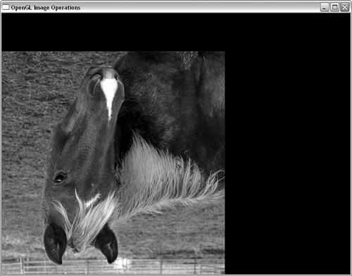
A negative zoom factor, on the other hand, has the effect of flipping the image along the direction of the zoom. Using such a zoom factor not only reverses the order of the pixels in the image, but also reverses the direction onscreen that the pixels are drawn with respect to the raster position. For example, normally an image is drawn with the lower-left corner being placed at the current raster position. If both zoom factors are negative, the raster position becomes the upper-right corner of the resulting image.
In the OPERATIONS sample program, selecting Flip Pixels inverts the image both horizontally and vertically. As shown in the following code snippet, the pixel zoom factors are both set to -1.0, and the raster position is changed from the lower-left corner of the window to a position that represents the upper-right corner of the image to be drawn (the image’s width and height):
case 2: // Flip the pixels
glPixelZoom(-1.0f, -1.0f);
glRasterPos2i(iWidth, iHeight);
break;
Figure 7.8 shows the inverted image when this option is selected.
Figure 7.8. Image displayed with x and y dimensions inverted.
Pixel Transfer
In addition to zooming pixels, OpenGL supports a set of simple mathematical operations that can be performed on image data as it is transferred either to or from the color buffer. These pixel transfer modes are set with one of the following functions and the pixel transfer parameters listed in Table 7.4:
void glPixelTransferi(GLenum pname, GLint param);
void glPixelTransferf(GLenum pname, GLfloat param);
Table 7.4. Pixel Transfer Parameters

The scale and bias parameters allow you to scale and bias individual color channels. A scaling factor is multiplied by the component value, and a bias value is added to that component value. A scale and bias operation is common in computer graphics for adjusting color channel values. The equation is simple:
New Value = (Old Value * Scale Value) + Bias Value
By default, the scale values are 1.0, and the bias values are 0.0. They essentially have no effect on the component values. Say you want to display a color image’s red component values only. To do this, you set the blue and green scale factors to 0.0 before drawing and back to 1.0 afterward:
glPixelTransferf(GL_GREEN_SCALE, 0.0f);
glPixelTransfer(GL_BLUE_SCALE, 0.0f);
The OPERATIONS sample program includes the menu selections Just Red, Just Green, and Just Blue, which demonstrate this particular example. Each selection turns off all but one color channel to show the image’s red, green, or blue color values only:
case 4: // Just Red
glPixelTransferf(GL_RED_SCALE, 1.0f);
glPixelTransferf(GL_GREEN_SCALE, 0.0f);
glPixelTransferf(GL_BLUE_SCALE, 0.0f);
break;
case 5: // Just Green
glPixelTransferf(GL_RED_SCALE, 0.0f);
glPixelTransferf(GL_GREEN_SCALE, 1.0f);
glPixelTransferf(GL_BLUE_SCALE, 0.0f);
break;
case 6: // Just Blue
glPixelTransferf(GL_RED_SCALE, 0.0f);
glPixelTransferf(GL_GREEN_SCALE, 0.0f);
glPixelTransferf(GL_BLUE_SCALE, 1.0f);
break;
After drawing, the pixel transfer for the color channels resets the scale values to 1.0:
glPixelTransferf(GL_RED_SCALE, 1.0f);
glPixelTransferf(GL_GREEN_SCALE, 1.0f);
glPixelTransferf(GL_BLUE_SCALE, 1.0f);
The post-convolution and post-color matrix scale and bias parameters perform the same operation but wait until after the convolution or color matrix operations have been performed. These operations are available in the imaging subset, which will be discussed shortly.
A more interesting example of the pixel transfer operations is to display a color image in black and white. The OPERATIONS sample does this when you choose the Black and White menu selection. First, the full-color image is drawn to the color buffer:
glDrawPixels(iWidth, iHeight, eFormat, GL_UNSIGNED_BYTE, pImage);
Next, a buffer large enough to hold just the luminance values for each pixel is allocated:
pModifiedBytes = (GLbyte *)malloc(iWidth * iHeight);
Remember, a luminance image has only one color channel, and here you allocate 1 byte (8 bits) per pixel. OpenGL automatically converts the image in the color buffer to luminance for use when you call glReadPixels but request the data be in the GL_LUMINANCE format:
glReadPixels(0,0,iWidth, iHeight, GL_LUMINANCE,
GL_UNSIGNED_BYTE, pModifiedBytes);
The luminance image can then be written back into the color buffer, and you would see the converted black-and-white image:
glDrawPixels(iWidth, iHeight, GL_LUMINANCE, GL_UNSIGNED_BYTE,
pModifiedBytes);
Using this approach sounds like a good plan, and it almost works. The problem is that when OpenGL converts a color image to luminance, it simply adds the color channels together. If the three color channels add up to a value greater than 1.0, it is simply clamped to 1.0. This has the effect of oversaturating many areas of the image. This effect is shown in Figure 7.9.
Figure 7.9. Oversaturation due to OpenGL’s default color-to-luminance operation.

To solve this problem, you must set the pixel transfer mode to scale the color value appropriately when OpenGL does the transfer from color to luminance colorspaces. According to the National Television Standards Committee (NTSC) standard, the conversion from RGB colorspace to black and white (grayscale) is
Luminance = (0.3 * Red) + (0.59 * Green) + (0.11 * Blue)
You can easily set up this conversion in OpenGL by calling these functions just before glReadPixels:
// Scale colors according to NTSC standard
glPixelTransferf(GL_RED_SCALE, 0.3f);
glPixelTransferf(GL_GREEN_SCALE, 0.59f);
glPixelTransferf(GL_BLUE_SCALE, 0.11f);
After reading pixels, you return the pixel transfer mode to normal:
// Return color scaling to normal
glPixelTransferf(GL_RED_SCALE, 1.0f);
glPixelTransferf(GL_GREEN_SCALE, 1.0f);
glPixelTransferf(GL_BLUE_SCALE, 1.0f);
The output is now a nice grayscale representation of the image. Because the figures in this book are not in color, but grayscale, the output onscreen looks exactly like the image in Figure 7.6. Color Plate 3 does, however, show the image (upper left) in full color, and the lower right in grayscale.
Pixel Mapping
In addition to scaling and bias operations, the pixel transfer operation also supports color mapping. A color map is a table used as a lookup to convert one color value (used as an index into the table) to another color value (the color value stored at that index). Color mapping has many applications, such as performing color corrections, making gamma adjustments, or converting to and from different color representations.
You’ll notice an interesting example in the OPERATIONS sample program when you select Invert Colors. In this case, a color map is set up to flip all the color values during a pixel transfer. This means all three channels are mapped from the range 0.0 to 1.0 to the range 1.0 to 0.0. The result is an image that looks like a photographic negative.
You enable pixel mapping by calling glPixelTransfer with the GL_MAP_COLOR parameter set to GL_TRUE:
glPixelTransferi(GL_MAP_COLOR, GL_TRUE);
To set up a pixel map, you must call another function, glPixelMap, and supply the map in one of three formats:
glPixelMapuiv(GLenum map, GLint mapsize, GLuint *values);
glPixelMapusv(GLenum map, GLint mapsize, GLushort *values);
glPixelMapfv(GLenum map, GLint mapsize, GLfloat *values);
The valid map values are listed in Table 7.5.
Table 7.5. Pixelmap Parameters

For the example, you set up a map of 256 floating-point values and fill the map with intermediate values from 1.0 to 0.0:
GLfloat invertMap[256];
...
...
invertMap[0] = 1.0f;
for(i = 1; i < 256; i++)
invertMap[i] = 1.0f - (1.0f / 255.0f * (GLfloat)i);
Then you set the red, green, and blue maps to this inversion map and turn on color mapping:
glPixelMapfv(GL_PIXEL_MAP_R_TO_R, 255, invertMap);
glPixelMapfv(GL_PIXEL_MAP_G_TO_G, 255, invertMap);
glPixelMapfv(GL_PIXEL_MAP_B_TO_B, 255, invertMap);
glPixelTransferi(GL_MAP_COLOR, GL_TRUE);
When glDrawPixels is called, the color components are remapped using the inversion table, essentially creating a color negative image. Figure 7.10 shows the output in black and white. Color Plate 3 in the Color insert shows a full-color image of this effect in the upper-right corner.
Figure 7.10. Using a color map to create a color negative image. (This figure also appears in the Color insert.)

The Imaging “Subset” and Pipeline
All the OpenGL functions covered so far in this chapter for image manipulation have been a part of the core OpenGL API since version 1.0. The only exception is the glWindowPos function, which was added in OpenGL 1.4 to make it easier to set the raster position. These features provide OpenGL with adequate support for most image manipulation needs. For more advanced imaging operations, OpenGL may also include, as of version 1.2, an imaging subset. The imaging subset is optional, which means vendors may choose not to include this functionality in their implementation. However, if the imaging subset is supported, it is an all-or-nothing commitment to support the entire functionality of these features.
Your application can determine at runtime whether the imaging subset is supported by searching the extension string for the token "GL_ARB_imaging". For example, when you use the glTools library, your code might look something like this:
if(gltIsExtSupported("GL_ARB_imaging") == 0)
{
// Error, imaging not supported
...
}
else
{
// Do some imaging stuff
...
...
}
You access the imaging subset through the OpenGL extension mechanism, which means you will likely need to use the glext.h header file and obtain function pointers for the functions you need to use. Some OpenGL implementations, depending on your platform’s development tools, may already have these functions and constants included in the gl.h OpenGL header file (for example, in the Apple XCode headers, they are already defined). For compiles on the Macintosh, we use the built-in support for the imaging subset; for other platforms, we use the extension mechanism to obtain function pointers to the imaging functions. This is all done transparently by adding glee.h and glee.c to your project. These files are located in the examples/src//shared directory in the source distribution for this book. It is safe to assume that you’ll need these files for most of the rest of the sample programs in this book.
The IMAGING sample program is modeled much like the previous OPERATIONS sample program in that a single sample program demonstrates different operations via the context menu. When the program starts, it checks for the availability of the imaging subset and aborts if it is not found:
// Check for imaging subset, must be done after window
// is created or there won't be an OpenGL context to query
if(gltIsExtSupported("GL_ARB_imaging") == 0)
{
printf("Imaging subset not supported
");
return 0;
}
The entire RenderScene function is presented in Listing 7.6. We discuss the various pieces of this function throughout this section.
Listing 7.6. The RenderScene Function from the Sample Program IMAGING

The image-processing subset can be broken down into three major areas of new functionality: the color matrix and color table, convolutions, and histograms. Bear in mind that image processing is a broad and complex topic all by itself and could easily warrant an entire book on this subject alone. What follows is an overview of this functionality with some simple examples of their use. For a more in-depth discussion on image processing, see the list of suggested references in Appendix A, “Further Reading/References.”
OpenGL imaging operations are processed in a specific order along what is called the imaging pipeline. In the same way that geometry is processed by the transformation pipeline, image data goes through the imaging operations in a fixed manner. Figure 7.11 breaks down the imaging pipeline operation by operation. The sections that follow describe these operations in more detail.
Figure 7.11. The OpenGL imaging pipeline.

Color Matrix
The simplest piece of new functionality added with the imaging subset is the color matrix. You can think of color values as coordinates in colorspace—RGB being akin to XYZ on the color axis of the color cube (described in Chapter 5, “Color, Materials, and Lighting: The Basics”). You could think of the alpha color component as the W component of a vector, and it would be transformed appropriately by a 4×4 color matrix. The color matrix is a matrix stack that works just like the other OpenGL matrix stacks (GL_MODELVIEW, GL_PROJECTION, GL_TEXTURE). You can make the color matrix stack the current stack by calling glMatrixMode with the argument GL_COLOR:
glMatrixMode(GL_COLOR);
All the matrix manipulation routines (glLoadIdentity, glLoadMatrix, and so on) are available for the color matrix. The color matrix stack can be pushed and popped as well, but implementations are required to support only a color stack two elements deep.
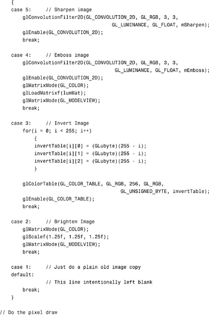
A menu item named Increase Contrast in the IMAGING sample program sets the render mode to 2, which causes the RenderScene function to use the color matrix to set a positive scaling factor to the color values, increasing the contrast of the image:
case 2: // Brighten Image
glMatrixMode(GL_COLOR);
glScalef(1.25f, 1.25f, 1.25f);
glMatrixMode(GL_MODELVIEW);
break;
The effect is subtle yet clearly visible when the change occurs onscreen. After rendering, the color matrix is restored to identity:
// Reset everything to default
glMatrixMode(GL_COLOR);
glLoadIdentity();
glMatrixMode(GL_MODELVIEW);
Color Lookup
With color tables, you can specify a table of color values used to replace a pixel’s current color. This functionality is similar to pixel mapping but has some added flexibility in the way the color table is composed and applied. The following function is used to set up a color table:
void glColorTable(GLenum target, GLenum internalFormat, GLsizei width,
GLenum format, GLenum type,
const GLvoid *table);
The target parameter specifies where in the imaging pipeline the color table is to be applied. This parameter may be one of the size values listed in Table 7.6.
Table 7.6. The Place to Apply the Color Lookup Table

You use the GL_PROXY prefixed targets to verify that the supplied color table can be loaded (will fit into memory).
The internalFormat parameter specifies the internal OpenGL representation of the color table pointed to by table. It can be any of the following symbolic constants: GL_ALPHA, GL_ALPHA4, GL_ALPHA8, GL_ALPHA12, GL_ALPHA16, GL_LUMINANCE, GL_LUMINANCE4, GL_LUMINANCE8, GL_LUMINANCE12, GL_LUMINANCE16, GL_LUMINANCE_ALPHA, GL_LUMINANCE4_ALPHA4, GL_LUMINANCE6_ALPHA2, GL_LUMINANCE8_ALPHA8, GL_LUMINANCE12_ALPHA4, GL_LUMINANCE12_ALPHA12, GL_LUMINANCE16_ALPHA16, GL_INTENSITY, GL_INTENSITY4, GL_INTENSITY8, GL_INTENSTIY12, GL_INTENSITY16, GL_RGB, GL_R3_G3_B2, GL_RGB4, GL_RGB5, GL_RGB8, GL_RGB10, GL_RGB12, GL_RGB16, GL_RGBA, GL_RGBA2, GL_RGBA4, GL_RGB5_A1, GL_RGBA8, GL_RGB10_A2, GL_RGBA12, GL_RGBA16. The color component name in this list should be fairly obvious to you by now, and the numerical suffix simply represents the bit count of that component’s representation.
The format and type parameters describe the format of the color table being supplied in the table pointer. The values for these parameters all correspond to the same arguments used in glDrawPixels, and are listed in Tables 7.2 and 7.3.
The following example demonstrates a color table in action. It duplicates the color inversion effect from the OPERATIONS sample program but uses a color table instead of pixel mapping. When you choose the Invert Color menu selection, the render mode is set to 3, and the following segment of the RenderScene function is executed:
case 3: // Invert Image
for(i = 0; i < 255; i++)
{
invertTable[i][0] = 255 - i;
invertTable[i][1] = 255 - i;
invertTable[i][2] = 255 - i;
}
glColorTable(GL_COLOR_TABLE, GL_RGB, 256, GL_RGB,
GL_UNSIGNED_BYTE, invertTable);
glEnable(GL_COLOR_TABLE);
For a loaded color table to be used, you must also enable the color table with a call to glEnable with the GL_COLOR_TABLE parameter. After the pixels are drawn, the color table is disabled:
glDisable(GL_COLOR_TABLE);
The output from this example matches exactly the image from Figure 7.10.
Proxies
An OpenGL implementation’s support for color tables may be limited by system resources. Large color tables, for example, may not be loaded if they require too much memory. You can use the proxy color table targets listed in Table 7.6 to determine whether a given color table fits into memory and can be used. These targets are used in conjunction with glGetColorTableParameter to see whether a color table will fit. The glGetColorTableParameter function enables you to query OpenGL about the various settings of the color tables; it is discussed in greater detail in Appendix C. Here, you can use this function to see whether the width of the color table matches the width requested with the proxy color table call:
GLint width;
...
...
glColorTable(GL_PROXY_COLOR_TABLE, GL_RGB, 256, GL_RGB,
GL_UNSIGNED_BYTE, NULL);
glGetColorTableParameteriv(GL_PROXY_COLOR_TABLE, GL_COLOR_TABLE_WIDTH, &width);
if(width == 0) {
// Error...
...
Note that you do not need to specify the pointer to the actual color table for a proxy.
Other Operations
Also in common with pixel mapping, the color table can be used to apply a scaling factor and a bias to color component values. You do this with the following function:
void glColorTableParameteriv(GLenum target, GLenum pname, GLint *param);
void glColorTableParameterfv(GLenum target, GLenum pname, GLfloat *param);
The glColorTableParameter function’s target parameter can be GL_COLOR_TABLE, GL_POST_CONVOLUTION_COLOR_TABLE, or GL_POST_COLOR_MATRIX_COLOR_TABLE. The pname parameter sets the scale or bias by using the value GL_COLOR_TABLE_SCALE or GL_COLOR_TABLE_BIAS, respectively. The final parameter is a pointer to an array of four elements storing the red, green, blue, and alpha scale or bias values to be used.
You can also actually render a color table by using the contents of the color buffer (after some rendering or drawing operation) as the source data for the color table. The function glCopyColorTable takes data from the current read buffer (the current GL_READ_BUFFER) as its source:
void glCopyColorTable(GLenum target, GLenum internalFormat,
GLint x, GLint y, GLsizei width);
The target and internalFormat parameters are identical to those used in glColorTable. The color table array is then taken from the color buffer starting at the x,y location and taking width pixels.
You can replace all or part of a color table by using the glColorSubTable function:
void glColorSubTable(GLenum target, GLsizei start, GLsizei count,
GLenum format, GLenum type, const void *data);
Here, most parameters correspond directly to the glColorTable function, except for start and count. The start parameter is the offset into the color table to begin the replacement, and count is the number of color values to replace.
Finally, you can also replace all or part of a color table from the color buffer in a manner similar to glCopyColorTable by using the glCopyColorSubTable function:
void glCopyColorSubTable(GLenum target, GLsizei start,
GLint x, GLint y, GLsizei width);
Again, the source of the color table is the color buffer, with x and y placing the position to begin reading color values, start being the location within the color table to begin the replacement, and width being the number of color values to replace.
Convolutions
Convolutions are a powerful image-processing technique, with many applications such as blurring, sharpening, and other special effects. A convolution is a filter that processes pixels in an image according to some pattern of weights called a kernel. The convolution replaces each pixel with the weighted average value of that pixel and its neighboring pixels, with each pixel’s color values being scaled by the weights in the kernel.
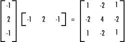
Typically, convolution kernels are rectangular arrays of floating-point values that represent the weights of a corresponding arrangement of pixels in the image. For example, the following kernel from the IMAGING sample program performs a sharpening operation:
static GLfloat mSharpen[3][3] = { // Sharpen convolution kernel
{0.0f, -1.0f, 0.0f},
{-1.0f, 5.0f, -1.0f },
{0.0f, -1.0f, 0.0f }};
The center pixel value is 5.0, which places a higher emphasis on that pixel value. The pixels immediately above, below, and to the right and left have a decreased weight, and the corner pixels are not accounted for at all. Figure 7.12 shows a sample block of image data with the convolution kernel superimposed. The 5 in the kernel’s center is the pixel being replaced, and you can see the kernel’s values as they are applied to the surrounding pixels to derive the new center pixel value (represented by the circle). The convolution kernel is applied to every pixel in the image, resulting in a sharpened image. You can see this process in action by selecting Sharpen Image in the IMAGING sample program.
Figure 7.12. The sharpening kernel in action.

To apply the convolution filter, the IMAGING program simply calls these two functions before the glDrawPixels operation:
glConvolutionFilter2D(GL_CONVOLUTION_2D, GL_RGB, 3, 3,
GL_LUMINANCE, GL_FLOAT, mSharpen);
glEnable(GL_CONVOLUTION_2D);
The glConvolutionFilter2D function has the following syntax:
void glConvolutionFilter2D(GLenum target, GLenum internalFormat,
GLsizei width, GLsizei height, GLenum format,
GLenum type, const GLvoid *image);
The first parameter, target, must be GL_CONVOLUTION_2D. The second parameter, internalFormat, takes the same values as glColorTable and specifies to which pixel components the convolution is applied. The width and height parameters are the width and height of the convolution kernel. Finally, format and type specify the format and type of pixels stored in image. In the case of the sharpening filter, the pixel data is in GL_RGB format, and the kernel is GL_LUMINANCE because it contains simply a single weight per pixel (as opposed to having a separate weight for each color channel). Convolution kernels are turned on and off simply with glEnable or glDisable and the parameter GL_CONVOLUTION_2D.
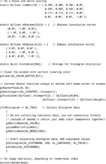
Convolutions are a part of the imaging pipeline and can be combined with other imaging operations. For example, the sharpening filter already demonstrated was used in conjunction with pixel zoom to fill the entire window with the image. For a more interesting example, let’s combine pixel zoom with the color matrix and a convolution filter. The following code excerpt defines a color matrix that will transform the image into a black-and-white (grayscale) image and a convolution filter that does embossing:

When you select Emboss Image from the pop-up menu, the render state is changed to 4, and the following case from the RenderScene function is executed before glDrawPixels:

The embossed image is displayed in Figure 7.13, and is shown in Color Plate 3 in the lower-left corner.
Figure 7.13. Using convolutions and the color matrix for an embossed effect.

From the Color Buffer
Convolution kernels can also be loaded from the color buffer. The following function behaves similarly to loading a color table from the color buffer:
void glCopyConvolutionFilter2D(GLenum target, GLenum internalFormat,
GLint x, GLint y, GLsizei width, GLsizei height);
The target value must always be GL_CONVOLUTION_2D, and internalFormat refers to the format of the color data, as in glConvolutionFilter2D. The kernel is loaded from pixel data from the color buffer located at (x,y) and the given width and height.
Separable Filters
A separable convolution filter is one whose kernel can be represented by the matrix outer product of two one-dimensional filters. For example, in Figure 7.14, one-dimensional row and column matrices are multiplied to yield a final 3×3 matrix (the new kernel filter).
Figure 7.14. The outer product to two one-dimensional filters.
The following function is used to specify these two one-dimensional filters:
void glSeparableFilter2D(GLenum target, GLenum internalFormat,
GLsizei width, GLsizei height,
GLenum format, GLenum type,
void *row, const GLvoid *column);
The parameters all have the same meaning as in glConvolutionFilter2D, with the exception that now you have two parameters for passing in the address of the filters: row and column. The target parameter, however, must be GL_SEPARABLE_2D in this case.
One-Dimensional Kernels
OpenGL also supports one-dimensional convolution filters, but they are applied only to one-dimensional texture data. They behave in the same manner as two-dimensional convolutions, with the exception that they are applied only to rows of pixels (or actually texels in the case of one-dimensional texture maps). These one-dimensional convolutions have one-dimensional kernels, and you can use the corresponding functions for loading and copying the filters:
glConvolutionFilter1D(GLenum target, GLenum internalFormat,
GLsizei width, GLenum format, GLenum type,
const GLvoid *image);
glCopyConvolutionFilter1D(GLenum target, GLenum internalFormat,
GLint x, GLint y, GLsizei width);
Of course, with these functions the target must be set to GL_CONVOLUTION_1D.
Other Convolution Tweaks
When a convolution filter kernel is applied to an image, along the edges of the image the kernel will overlap and fall outside the image’s borders. How OpenGL handles this situation is controlled via the convolution border mode. You set the convolution border mode by using the glConvolutionParameter function, which has four variations:
glConvolutionParameteri(GLenum target, GLenum pname, GLint param);
glConvolutionParameterf(GLenum target, GLenum pname, GLfloat param);
glConvolutionParameteriv(GLenum target, GLenum pname, GLint *params);
glConvolutionParameterfv(GLenum target, GLenum pname, GLfloat *params);
The target parameter for these functions can be GL_CONVOLUTION_1D, GL_CONVOLUTION_2D, or GL_SEPARABLE_2D. To set the border mode, you use GL_CONVOLUTION_BORDER_MODE as the pname parameter and one of the border mode constants as param.
If you set param to GL_CONSTANT_BORDER, the pixels outside the image border are computed from a constant pixel value. To set this pixel value, call glConvolutionParameterfv with GL_CONSTANT_BORDER and a floating-point array containing the RGBA values to be used as the constant pixel color.
If you set the border mode to GL_REDUCE, the convolution kernel is not applied to the edge pixels. Thus, the kernel never overlaps the edge of the image. In this case, however, you should note that you are essentially shrinking the image by the width and height of the convolution filter.
The final border mode is GL_REPLICATE_BORDER. In this case, the convolution is applied as if the horizontal and vertical edges of an image are replicated as many times as necessary to prevent overlap.
You can also apply a scale and bias value to kernel values by using GL_CONVOLUTION_FILTER_BIAS and/or GL_CONVOLUTION_FILTER_SCALE for the parameter name (pname) and supplying the bias and scale values in param or params.
Histogram
A histogram is a graphical representation of an image’s frequency distribution. In English, it is simply a count of how many times each color value is used in an image, displayed as a sort of bar graph. Histograms may be collected for an image’s intensity values or separately for each color channel. Histograms are frequently employed in image processing, and many digital cameras can display histogram data of captured images. Photographers use this information to determine whether the camera captured the full dynamic range of the subject or if perhaps the image is too over- or underexposed. Popular image-processing packages such as Adobe Photoshop also calculate and display histograms, as shown in Figure 7.15.
Figure 7.15. A histogram display in Photoshop.

When histogram collection is enabled, OpenGL collects statistics about any images as they are written to the color buffer. To prepare to collect histogram data, you must tell OpenGL how much data to collect and in what format you want the data. You do this with the glHistogram function:
void glHistogram(GLenum target, GLsizei width,
GLenum internalFormat, GLboolean sink);
The target parameter must be either GL_HISTOGRAM or GL_PROXY_HISTOGRAM (used to determine whether sufficient resources are available to store the histogram). The width parameter tells OpenGL how many entries to make in the histogram table. This value must be a power of 2 (1, 2, 4, 8, 16, and so on). The internalFormat parameter specifies the data format you expect the histogram to be stored in, corresponding to the valid format parameters for color tables and convolution filters, with the exception that GL_INTENSITY is not included. Finally, you can discard the pixels and not draw anything by specifying GL_TRUE for the sink parameter. You can turn histogram data collection on and off with glEnable or glDisable by passing in GL_HISTOGRAM, as in this example:
glEnable(GL_HISTOGRAM);
After image data has been transferred, you collect the histogram data with the following function:
void glGetHistogram(GLenum target, GLboolean reset, GLenum format,
GLenum type, GLvoid *values);
The only valid value for target is GL_HISTOGRAM. Setting reset to GL_TRUE clears the histogram data. Otherwise, the histogram becomes cumulative, and each pixel transfer continues to accumulate statistical data in the histogram. The format parameter specifies the data format of the collected histogram information, and type and values are the data type to be used and the address where the histogram is to be placed.
Now, let’s look at an example using a histogram. In the IMAGING sample program, selecting Histogram from the menu displays a grayscale version of the image and a graph in the lower-left corner that represents the statistical frequency of each color luminance value. The output is shown in Figure 7.16.
Figure 7.16. A histogram of the luminance values of the image.

The first order of business in the RenderScene function is to allocate storage for the histogram. The following line creates an array of integers 256 elements long. Each element in the array contains a count of the number of times that corresponding luminance value was used when the image was drawn onscreen:
static GLint histoGram[256]; // Storage for histogram statistics
Next, if the histogram flag is set (through the menu selection), you tell OpenGL to begin collecting histogram data. The function call to glHistogram instructs OpenGL to collect statistics about the 256 individual luminance values that may be used in the image. The sink is set to false so that the image is also drawn onscreen:
if(bHistogram == GL_TRUE) // Collect Histogram data
{
// We are collecting luminance data, use our conversion formula
// instead of OpenGL's (which just adds color components together)
glMatrixMode(GL_COLOR);
glLoadMatrixf(lumMat);
glMatrixMode(GL_MODELVIEW);
// Start collecting histogram data, 256 luminance values
glHistogram(GL_HISTOGRAM, 256, GL_LUMINANCE, GL_FALSE);
glEnable(GL_HISTOGRAM);
}
Note that in this case you also need to set up the color matrix to provide the grayscale color conversion. OpenGL’s default conversion to GL_LUMINANCE is simply a summing of the red, green, and blue color components. When you use this conversion formula, the histogram graph will have the same shape as the one from Photoshop for the same image displayed in Figure 7.15.
After the pixels are drawn, you collect the histogram data with the code shown here:
// Fetch and draw histogram?
if(bHistogram == GL_TRUE)
{
// Read histogram data into buffer
glGetHistogram(GL_HISTOGRAM, GL_TRUE, GL_LUMINANCE, GL_INT, histoGram);
Now you traverse the histogram data and search for the largest collected value. You do this because you will use this value as a scaling factor to fit the graph in the lower-left corner of the display:
// Find largest value for scaling graph down
GLint iLargest = 0;
for(i = 0; i < 255; i++)
if(iLargest < histoGram[i])
iLargest = histoGram[i];
Finally, it’s time to draw the graph of statistics. The following code segment simply sets the drawing color to white and then loops through the histogram data creating a single line strip. The data is scaled by the largest value so that the graph is 256 pixels wide and 128 pixels high. When all is done, the histogram flag is reset to false and the histogram data collection is disabled with a call to glDisable:
// White lines
glColor3f(1.0f, 1.0f, 1.0f);
glBegin(GL_LINE_STRIP);
for(i = 0; i < 255; i++)
glVertex2f((GLfloat)i, (GLfloat)histoGram[i] /
(GLfloat) iLargest * 128.0f);
glEnd();
bHistogram = GL_FALSE;
glDisable(GL_HISTOGRAM);
}
Minmax Operations
In the preceding sample, you traversed the histogram data to find the largest luminance component for the rendered image. If you need only the largest or smallest components collected, you can choose not to collect the entire histogram for a rendered image, but instead collect the largest and smallest values. This minmax data collection operates in a similar manner to histograms. First, you specify the format of the data on which you want statistics gathered by using the following function:
void glMinmax(GLenum target, GLenum internalFormat, GLboolean sink);
Here, target is GL_MINMAX, and internalFormat and sink behave precisely as in glHistogram. You must also enable minmax data collection:
glEnable(GL_MINMAX);
The minmax data is collected with the glGetMinmax function, which is analogous to glGetHistogram:
void glGetMinmax(GLenum target, GLboolean reset, GLenum format,
GLenum type, GLvoid *values);
Again, the target parameter is GL_MINMAX, and the other parameters map to their counterparts in glGetHistogram.
Summary
In this chapter, we have shown that OpenGL provides first-class support for color image manipulation—from reading and writing bitmaps and color images directly to the color buffer, to color processing operations and color lookup maps. Optionally, many OpenGL implementations go even further by supporting the OpenGL imaging subset. The imaging subset makes it easy to add sophisticated image-processing filters and analysis to your graphics-intensive programs.
We have also laid the groundwork in this chapter for our return to 3D geometry in the next chapter, where we begin coverage of OpenGL’s texture mapping capabilities. You’ll find that the functions covered in this chapter that load and process image data are used directly when we extend the manipulation of image data by mapping it to 3D primitives.