Description of Shortest Paths
Finding the shortest path, or minimum-weight path, from one vertex to another in a graph is an important distillation of many routing problems. Formally stated, given a directed, weighted graph G = (V, E ), the shortest path from vertex s to t in V is the set S of edges in E that connect s to t at a minimum cost.
When we find S, we are solving the single-pair shortest-path problem. To do this, in actuality we solve the more general single-source shortest-paths problem , which solves the single-pair shortest-path problem in the process. In the single-source shortest-paths problem, we compute the shortest paths from a start vertex s to all other vertices reachable from it. We solve this problem because no algorithm is known to solve the single-pair shortest-path problem any faster.
Dijkstra’s Algorithm
One approach to solving the single-source shortest-paths problem is Dijkstra’s algorithm (pronounced “Dikestra”). Dijkstra’s algorithm grows a shortest-paths tree, whose root is the start vertex s and whose branches are the shortest paths from s to all other vertices in G. The algorithm requires that all weights in the graph be nonnegative. Like Prim’s algorithm, Dijkstra’s algorithm is another example of a greedy algorithm that happens to produce an optimal result. The algorithm is greedy because it adds edges to the shortest-paths tree based on which looks best at the moment.
Fundamentally, Dijkstra’s algorithm works by repeatedly selecting a vertex and exploring the edges incident from it to determine whether the shortest path to each vertex can be improved. The algorithm resembles a breadth-first search because it explores all edges incident from a vertex before moving deeper in the graph. To compute the shortest paths between s and all other vertices, Dijkstra’s algorithm requires that a color and shortest-path estimate be maintained with every vertex. Typically, shortest-path estimates are represented by the variable d.
Initially, we set all colors to white, and we set all shortest-path estimates to ∞, which represents an arbitrarily large value greater than the weight of any edge in the graph. We set the shortest-path estimate of the start vertex to 0. As the algorithm progresses, we assign to all vertices except the start vertex a parent in the shortest-paths tree. The parent of a vertex may change several times before the algorithm terminates.
Dijkstra’s algorithm proceeds as follows. First, from among all white vertices in the graph, we select the vertex u with the smallest shortest-path estimate. Initially, this will be the start vertex since its shortest-path estimate is 0. After we select the vertex, we color it black. Next, for each white vertex v adjacent to u, we relax the edge (u, v). When we relax an edge, we determine whether going through u improves the shortest path computed thus far to v. To make this decision, we add the weight of (u, v) to the shortest-path estimate for u. If this value is less than or equal to the shortest-path estimate for v, we assign the value to v as its new shortest-path estimate, and we set the parent of v to u. We then repeat this process until all vertices have been colored black. Once we have computed the shortest-paths tree, the shortest path from s to another vertex t can be determined by starting at t in the tree and following successive parents until we reach s. The path in reverse is the shortest path from s to t.
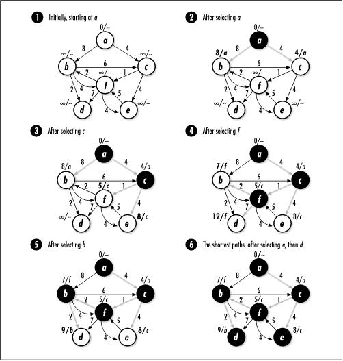
Figure 16.3 illustrates the computation of the shortest paths between a and all other vertices in the graph. The shortest path from a to b, for example, is 〈 a, c, f, b 〉, which has a total weight of 7. The shortest-path estimate and parent of each vertex are displayed beside the vertex. The shortest-path estimate is to the left of the slash, and the parent is to the right. The edges shaded in light gray are the edges in the shortest-paths tree as it changes.