To begin, let’s consider a simple problem that normally we might not think of in a recursive way. Suppose we would like to compute the factorial of a number n. The factorial of n, written n!, is the product of all numbers from n down to 1. For example, 4! = (4)(3)(2)(1). One way to calculate this is to loop through each number and multiply it with the product of all preceding numbers. This is an iterative approach, which can be defined more formally as:

n! = (n)(n - 1)(n - 2) . . . (1)

Another way to look at this problem is to define n! as the product of smaller factorials. To do this, we define n! as n times the factorial of n - 1. Of course, solving (n - 1)! is the same problem as n!, only a little smaller. If we then think of (n - 1)! as n - 1 times (n - 2)!, (n - 2)! as n - 2 times (n - 3)!, and so forth until n = 1, we end up computing n!. This is a recursive approach, which can be defined more formally as:

Figure 3.1 illustrates computing 4! using the recursive approach just described. It also delineates the two basic phases of a recursive process: winding and unwinding . In the winding phase, each recursive call perpetuates the recursion by making an additional recursive call itself. The winding phase terminates when one of the calls reaches a terminating condition. A terminating condition defines the state at which a recursive function should return instead of making another recursive call. For example, in computing the factorial of n, the terminating conditions are n = 1 and n = 0, for which the function simply returns 1. Every recursive function must have at least one terminating condition; otherwise, the winding phase never terminates. Once the winding phase is complete, the process enters the unwinding phase, in which previous instances of the function are revisited in reverse order. This phase continues until the original call returns, at which point the recursive process is complete.

Figure 3.1. Computing 4! recursively

Example 3.1 presents a C function, fact, that accepts a number n and computes its factorial recursively. The function works as follows. If n is less than 0, the function returns 0, indicating an error. If n is or 1, the function returns 1 because 0! and 1! are both defined as 1. These are the terminating conditions. Otherwise, the function returns the result of n times the factorial of n - 1. The factorial of n - 1 is computed recursively by calling fact again, and so forth. Notice the similarities between this implementation and the recursive definition shown earlier.

/*****************************************************************************
*                                                                            *
*  -------------------------------- fact.c --------------------------------  *
*                                                                            *
*****************************************************************************/

#include "fact.h"

/*****************************************************************************
*                                                                            *
*  --------------------------------- fact ---------------------------------  *
*                                                                            *
*****************************************************************************/

int fact(int n) {

/*****************************************************************************
*                                                                            *
*  Compute a factorial recursively.                                          *
*                                                                            *
*****************************************************************************/

if (n < 0)
   return 0;
else if (n == 0)
   return 1;
else if (n == 1)
   return 1;
else
   return n * fact(n - 1);

}

To understand how recursion really works, it helps to look at the way functions are executed in C. For this, we need to understand a little about the organization of a C program in memory. Fundamentally, a C program consists of four areas as it executes: a code area, a static data area, a heap, and a stack (see Figure 3.2a). The code area contains the machine instructions that are executed as the program runs. The static data area contains data that persists throughout the life of the program, such as global variables and static local variables. The heap contains dynamically allocated storage, such as memory allocated by malloc. The stack contains information about function calls. By convention, the heap grows upward from one end of a program’s memory, while the stack grows downward from the other (but this may vary in practice). Note that the term heap as it is used in this context has nothing to do with the heap data structure presented in Chapter 10.

When a function is called in a C program, a block of storage is allocated on the stack to keep track of information associated with the call. Each call is referred to as an activation. The block of storage placed on the stack is called an activation record or, alternatively, a stack frame. An activation record consists of five regions: incoming parameters, space for a return value, temporary storage used in evaluating expressions, saved state information for when the activation terminates, and outgoing parameters (see Figure 3.2b). Incoming parameters are the parameters passed into the activation. Outgoing parameters are the parameters passed to functions called within the activation. The outgoing parameters of one activation record become the incoming parameters of the next one placed on the stack. The activation record for a function call remains on the stack until the call terminates.

Returning to Example 3.1, consider what happens on the stack as one computes 4!. The initial call to fact results in one activation record being placed on the stack with an incoming parameter of n = 4 (see Figure 3.3, step 1). Since this activation does not meet any of the terminating conditions of the function, fact is recursively called with n set to 3. This places another activation of fact on the stack, but with an incoming parameter of n = 3 (see Figure 3.3, step 2). Here, n = 3 is also an outgoing parameter of the first activation since the first activation invoked the second. The process continues this way until n is 1, at which point a terminating condition is encountered and fact returns 1 (see Figure 3.3, step 4).

Figure 3.2. The organization in memory of (a) a C program and (b) an activation record

Figure 3.3. The stack of a C program while computing 4! recursively

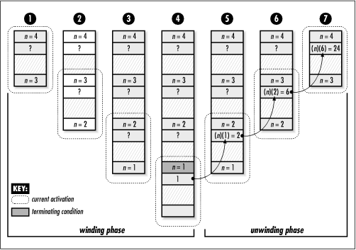
Once the n = 1 activation terminates, the recursive expression in the n = 2 activation is evaluated as (2)(1) = 2. Thus, the n = 2 activation terminates with a return value of 2 (see Figure 3.3, step 5). Consequently, the recursive expression in the n = 3 activation is evaluated as (3)(2) = 6, and the n = 3 activation returns 6 (see Figure 3.3, step 6). Finally, the recursive expression in the n = 4 activation is evaluated as (4)(6) = 24, and the n = 4 activation terminates with a return value of 24 (see Figure 3.3, step 7). At this point, the function has returned from the original call, and the recursive process is complete.

The stack is a great solution to storing information about function calls because its last-in, first-out behavior (see Chapter 6) is well suited to the order in which functions are called and terminated. However, stack usage does have a few drawbacks. Maintaining information about every function call until it returns takes a considerable amount of space, especially in programs with many recursive calls. In addition, generating and destroying activation records takes time because there is a significant amount of information that must be saved and restored. Thus, if the overhead associated with these concerns becomes too great, we may need to consider an iterative approach. Fortunately, we can use a special type of recursion, called tail recursion, to avoid these concerns in some cases.