![]()
Storage Indexes
Storage indexes are a useful Exadata feature that you never hear about. They are not indexes that are stored in the database like Oracle’s traditional B-tree or bitmapped indexes. In fact, they are not indexes at all in the traditional sense. They are not capable of identifying a set of records that has a certain value in a given column. Rather, they are a feature of the storage server software that is designed to eliminate disk I/O. They are sometimes described as “reverse indexes.” That’s because they identify locations where the requested records are not, instead of the other way around. They work by storing minimum and maximum values and the existence of null values for a column for disk storage units, which are 1 megabyte (MB) by default. Because SQL predicates are passed to the storage servers when Smart Scans are performed, the storage software can check the predicates against the storage index metadata (maximum, minimum, null values) before doing the requested I/O. Any storage region that cannot possibly have a matching row is skipped. In many cases, this can result in a significant reduction in the amount of I/O that must be performed. Keep in mind that since the storage software needs the predicates to compare to the maximum and minimum values and/or null in the storage indexes, this optimization is only available for Smart Scans.
The storage software provides no documented mechanism for altering or tuning storage indexes (although there are a few undocumented parameters that can be set prior to starting cellsrv on the storage servers). In fact, there is not even much available in the way of monitoring. For example, there is no wait event that records the amount of time spent when a storage index is accessed or updated. Even though there are no documented commands to manipulate storage indexes, they are an extremely powerful feature and can provide dramatic performance improvements. For that reason, it is important to understand how they work.
Storage indexes consist of a minimum and a maximum value and the existence of null for up to eight columns. This structure is maintained for 1MB chunks of storage (storage regions) by default. Storage indexes are stored in memory only and are never written to disk.
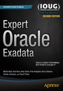
Figure 4-1 shows a conceptual view of the data contained in a storage index.
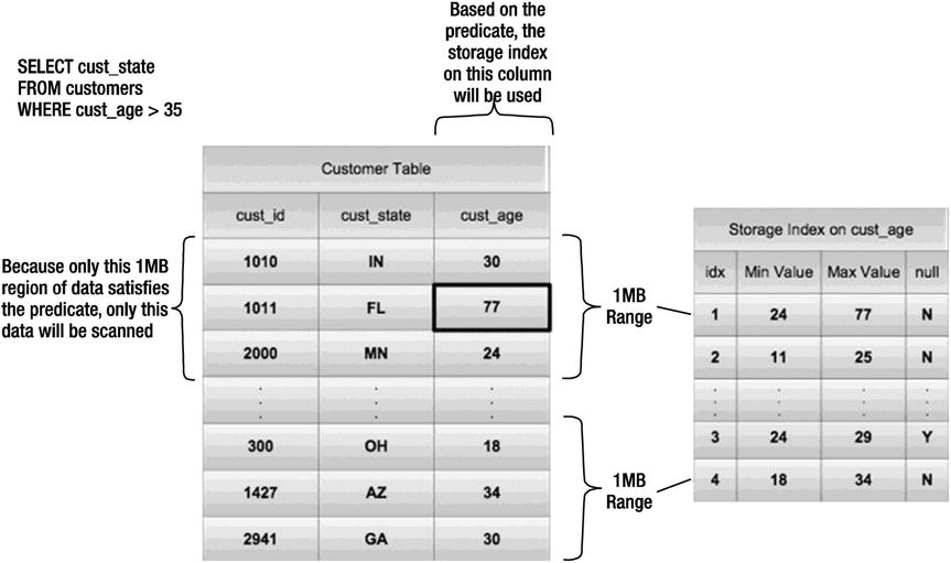
Figure 4-1. Conceptual diagram of a storage index
As you can see in the diagram, the first storage region in the customer table has a maximum value of 77, indicating that it’s possible for it to contain rows that will satisfy the query predicate (cust_age >35). The other storage regions in the diagram do not have maximum values that are high enough to contain any records that will satisfy the query predicate. Therefore, those storage regions will not be read from disk.
In addition to the minimum and maximum values, there is a flag to indicate whether any of the records in a storage region contain nulls. The fact that nulls are represented at all is somewhat surprising given that nulls are not stored in traditional Oracle indexes. This ability of storage indexes to track nulls may actually have repercussions for design and implementation decisions. There are systems that don’t use nulls at all. SAP, for example, uses a single space character instead of nulls. SAP does this simply to insure that records can be accessed via B-tree indexes (which do not store nulls). At any rate, storage indexes provide the equivalent of a bitmapped index on nulls, which makes finding nulls a very efficient process (assuming they represent a low percentage of the values).
Monitoring Storage Indexes
The ability to monitor storage indexes is very limited. The optimizer does not know whether a storage index will be used for a particular SQL statement. Nor do AWR or ASH capture any information about whether storage indexes were used by particular SQL statements. There is a single statistic that reports storage index usage at the database level and an undocumented tracing mechanism.
Database Statistics
There is only one database statistic directly related to storage indexes. The statistic, cell physical IO bytes saved by storage index, keeps track of the accumulated I/O that has been avoided by the use of storage indexes. This statistic is exposed in v$sesstat and v$sysstat and related views. It’s a strange statistic that calculates a precise value for something it didn’t do. Nevertheless, it is the only easily accessible indicator as to whether storage indexes have been used. Unfortunately, since the statistic is cumulative like all statistics in v$sesstat, it must be checked before and after a given SQL statement in order to determine whether storage indexes were used on that particular statement. Here is an example:
KSO@dbm2> select name, value
  2       from v$mystat s, v$statname n
  3       where s.statistic# = n.statistic#
  4       and name like '%storage index%';

NAME                                                                  VALUE
---------------------------------------------------------------- ----------
cell physical IO bytes saved by storage index                             0

KSO@dbm2> select avg(pk_col) from kso.skew2 where col1 is null;

AVG(PK_COL)
-----------
   32000001

KSO@dbm2> select name, value
  2  from v$mystat s, v$statname n
  3  where s.statistic# = n.statistic#
  4  and name like '%storage index%';

NAME                                                                  VALUE
---------------------------------------------------------------- ----------
cell physical IO bytes saved by storage index                    1842323456
As you can see, the first query asks v$mystat for a statistic that contains the term storage index. The value for this statistic will be 0 until a SQL statement that uses a storage index has been executed in the current session. In our example, the query used a storage index that eliminated about 1.8 gigabytes of disk I/O. This is the amount of additional I/O that would have been necessary without storage indexes. Note that v$mystat is a view that exposes cumulative statistics for your current session. As a result, if you run the statement a second time, the value should increase to twice the value it had after the first execution. Of course, disconnecting from the session (by exiting SQL*Plus, for example) resets most statistics exposed by v$mystat, including this one, to 0.
There is another way to monitor what is going on with storage indexes at the individual storage cell level. The cellsrv program has the ability to create trace files whenever storage indexes are accessed. This tracing can be enabled by setting the _CELL_STORAGE_INDEX_DIAG_MODE parameter to 2 either in the cellinit.ora file to make the setting consistent across restarts of the cell server, or by changing the parameter on runtime in a cell server using the following code:
CellCLI> alter cell events="immediate cellsrv.cellsrv_setparam('_cell_storage_index_diag_mode',2)"
CELLSRV parameter changed: _cell_storage_index_diag_mode=2.
Modification is in-memory only.
Add parameter setting to 'cellinit.ora' if the change needs to be persistent across cellsrv reboots.
Cell enkx4cel02 successfully altered"
During normal use, it is obvious this parameter should be set to 0 to prevent the storage cell from the overhead of writing trace files. To make sure this parameter is set to the correct value, it can be queried from storage cell using the following:
CellCLI> alter cell events="immediate cellsrv.cellsrv_getparam('_cell_storage_index_diag_mode')
Parameter _cell_storage_index_diag_mode has value 0
Cell enkx4cel01 successfully altered
Tracing can also be enabled on all storage servers for SQL using storage indexes by setting the hidden database parameter, _KCFIS_STORAGEIDX_DIAG_MODE to a value of 2. Since these tracing mechanisms are completely undocumented, it should not be used without approval from Oracle support. Better safe than sorry.
Because the cellsrv process is multithreaded, the tracing facility creates many trace files. The result is similar to tracing a select statement that is executed in parallel on a database server in that there are multiple trace files that need to be combined to show the whole picture. The naming convention for the trace files is svtrc_, followed by a process ID, followed by a thread identifier. The process ID matches the operating system process ID of the cellsrv process. Since cellsrv enables only 100 threads by default (_CELL_NUM_THREADS), the file names are reused rapidly as requests come into the storage cells. Because of this rapid reuse, it’s quite easy to wrap around the thread number portion of the file name. Such wrapping around does not wipe out the previous trace file, but rather appends new data to the existing file. Appending happens with trace files on Oracle database servers as well, but is much less common because the process ID portion of the default file name comes from the user’s shadow process. By using the process ID as the identifier for the trace file with the database server, basically each session gets its own number.
Starting from the 12c release of of the storage cell software, Oracle created the concept of offload servers for the cell storage server. A cell offload server is a distinct (threaded) process started by the main cell server to have the ability to run different versions of the storage server software at the same time. The trace files that contain the information generated using above mentioned methods are the trace files generated by the offload server, not the main cell server. This also changes the trace file name—the start of the trace file name starts with cellofltrc_, and the offload server has its own diagnostic destination.
There is another related cellsrv parameter, _CELL_SI_MAX_NUM_DIAG_MODE_DUMPS, that sets a maximum number of trace files that will be created before the tracing functionality is turned off. The parameter defaults to a value of 20. Presumably, the parameter is a safety mechanism to keep the disk from getting filled by trace files since a single query can create a large number of files.
Here is a snippet from a trace file generated on our test system:
Trace file /opt/oracle/cell/log/diag/asm/cell/SYS_121111_140712/trace/cellofltrc_16634_15.trc
ORACLE_HOME = /opt/oracle/cell/cellofl-12.1.1.1.1_LINUX.X64_140712
System name:    Linux
Node name:      enkx4cel01.enkitec.com
Release:        2.6.39-400.128.17.el5uek
Version:        #1 SMP Tue May 27 13:20:24 PDT 2014
Machine:        x86_64
CELL SW Version:        OSS_12.1.1.1.1_LINUX.X64_140712
CELLOFLSRV SW Version:  OSS_12.1.1.1.1_LINUX.X64_140712


*** 2015-01-25 05:42:43.299
UserThread: LWPID: 16684 userId: 15 kernelId: 15 pthreadID: 140085391522112
*** 2015-01-25 06:38:55.655
4220890033:2 SIerr=0 size=1048576
2015-01-25 06:38:55.655743 :000031DA: ocl_si_ridx_pin: Pin successful for rgn_hdl:0x6000116c1d28 rgn_index:10206 rgn_hdr:0x600085fd2de4 group_id:2 si_ridx:0x6000aa687930
4220890033:2 SIerr=0 size=1048576
2015-01-25 06:38:55.655774 :000031DB: ocl_si_ridx_pin: Pin successful for rgn_hdl:0x6000116c1d28 rgn_index:10207 rgn_hdr:0x600085fd2df4 group_id:2 si_ridx:0x6000aa687a18
4220890033:2 SIerr=0 size=1048576
2015-01-25 06:38:55.655801 :000031DC: ocl_si_ridx_pin: Pin successful for rgn_hdl:0x6000116c3048 rgn_index:10240 rgn_hdr:0x60008eff7004 group_id:2 si_ridx:0x6000aa687db8
4220890033:2 SIerr=0 size=1015808
2015-01-25 06:38:55.655828 :000031DD: ocl_si_ridx_pin: Pin successful for rgn_hdl:0x6000116c3048 rgn_index:10241 rgn_hdr:0x60008eff7014 group_id:2 si_ridx:0x6000aa687b00
Several things are worth pointing out in this trace file:
- The first several lines are the standard trace file header with file name and software version.
- The (default) storage index tracing does contain a lot less information than used to be shown in previous (11g) versions of the storage server software, before the existence of offload servers.
- Every storage index entry describes a region of mostly 1048576 bytes (size=1048576).
- For every storage index entry used, the entry is “pinned” to guarantee the entry not being removed of modified during usage (ocl_si_ridx_pin).
For the sake of completeness, a dump of a storage index has been performed on version 11.2.3.3.1 of the storage server. The reason for using version 11 is that starting from version 12, the storage server will skip dumping the actual storage index, as can be seen in the previous dump. The 11.2.3.3.1 dump shows an actual storage index for one storage region:
2015-01-31 05:58:14.530028*: RIDX(0x7f07556eb1c0) : st 2(RIDX_VALID) validBitMap 0 tabn 0 id {6507 1 964151215}
2015-01-31 05:58:14.530028*: RIDX: strt 32 end 2048 offset 86312501248 size 1032192 rgnIdx 82314 RgnOffset 16384 scn: 0x0000.00e9aa10 hist: 1
2015-01-31 05:58:14.530028*: RIDX validation history:
2015-01-31 05:58:14.530028*: 0:PartialRead 1:Undef 2:Undef 3:Undef 4:Undef 5:Undef 6:Undef 7:Undef 8:Undef 9:Undef
2015-01-31 05:58:14.530028*: Col id [1] numFilt 5 flg 2 (HASNONNULLVALUES):
2015-01-31 05:58:14.530028*: lo: c2 16 64 0 0 0 0 0
2015-01-31 05:58:14.530028*: hi: c2 19 8 0 0 0 0 0
2015-01-31 05:58:14.530028*: Col id [2] numFilt 4 flg 2 (HASNONNULLVALUES):
2015-01-31 05:58:14.530028*: lo: c5 15 4d c 22 26 0 0
2015-01-31 05:58:14.530028*: hi: c5 15 4d c 22 26 0 0
2015-01-31 05:58:14.530028*: Col id [7] numFilt 4 flg 2 (HASNONNULLVALUES):
2015-01-31 05:58:14.530028*: lo: c1 3 0 0 0 0 0 0
2015-01-31 05:58:14.530028*: hi: c1 3 0 0 0 0 0 0
The following items are worth pointing out:
- The storage index entry describes a region close to 1MB (size=1032192).
- It looks like this Storage Index entry occupies 2K of memory based on the strt and end field values.
- For each column evaluated, there is an id field that correlates to its position in the table.
- For each column evaluated, there is a flg field. It appears that it is the decimal representation of a bit mask. It also appears that the first bit indicates whether nulls are contained in the current column of the storage region. (That is, 1 and 3 both indicate that nulls are present.)
- For each column evaluated, there is a lo and a hi value (stored as hex).
- The lo and hi values are only eight bytes, indicating that the storage indexes will be ineffective on columns where the leading portion of the values are not distinct (empirical evidence bears this out, by the way).
While generating and reading trace files is very informative, it is not very easy to do and requires direct access to the storage servers. On top of that, the approach is completely undocumented. It is probably best used for investigations in nonproduction environments.
Monitoring Wrap-Up
Neither the database statistic nor the tracing is a particularly satisfying way of monitoring storage index usage. It would be nice to be able to track storage index usage at the statement level via a column in V$SQL, for example. In the meantime, the cell physical IO bytes saved by storage index statistic is the best option we have.
There is not much you can do to control storage index behavior. However, the developers have built in a few hidden parameters that provide some flexibility.
There are four database parameters that deal with storage indexes (that we’re aware of):
- _kcfis_storageidx_disabled (default is FALSE)
- _kcfis_storageidx_diag_mode (default is 0)
- _cell_storidx_mode (default is EVA)
- _cell_storidx_minmax_enabled (default is TRUE)
None of these parameters are documented, so you need to be careful with the methods we discuss in this section. Nevertheless, we will tell you a little bit about some of these parameters and what they can do.
The _kcfis_storageidx_disabled parameter allows storage indexes to be disabled. As with all hidden parameters, it’s best to check with Oracle support before setting it, but as hidden parameters go, this one is relatively innocuous. We have used it extensively in testing and have not experienced any negative consequences.
You can set the parameter at the session level with the alter session statement:
alter session set "_kcfis_storageidx_disabled"=true;
Note that although setting _kcfis_storageidx_disabled to TRUE disables storage indexes for reads, the setting does not disable the maintenance of existing storage indexes. That is to say that existing storage indexes will still be updated when values in a table are changed, even if this parameter is set to TRUE.
The second parameter, __KCFIS_STORAGEIDX_DIAG_MODE, looks eerily like the cellinit.ora parameter _CELL_STORAGE_INDEX_DIAG_MODE, which was discussed earlier. As you might expect, setting this parameter at the database layer causes trace files to be generated across all the affected storage cells. Setting it to a value of 2 enables tracing. Oddly, setting it to a value of 1 disables storage indexes. Unfortunately, the trace files are created on the storage cells, but this method of generating them is much less intrusive than restarting the cellsrv process on a storage server.
You can set the parameter at the session level with the alter session statement:
alter session set "_kcfis_storageidx_diag_mode"=2;
There may be other valid values for the parameter that enable different levels of tracing. Keep in mind that this will produce a large number of trace files on every storage cell that is involved in a query that uses storage indexes.
The _CELL_STORIDX_MODE parameter was added in the second point release of Oracle Database 11gR2 (11.2.0.2). While this parameter is undocumented, it appears that it controls where storage indexes will be applied. There are three valid values for this parameter (EVA,KDST,ALL). EVA and KDST are Oracle kernel function names.
You can set the parameter at the session level with the alter session statement:
alter session set "_cell_storidx_mode"=ALL;
The effects of this parameter have varied across releases. As of cellsrv version 11.2.2.3.0, EVA (the default) supports all the valid comparison operators. You should note that in older versions, the EVA setting did not support the IS NULL comparison operator. It’s also important to keep in mind that the database patching is tied to the storage software patching. Upgrading the version of cellsrv without patching the database software can result in unpredicatable behavior (disabling storage indexes, for example).
The _CELL_STORIDX_MINMAX_ENABLED parameter was added in the 12.1.0.2 release of Oracle Database. The default value is TRUE.
This parameter controls a new feature in cellsrv version 12.1.2.1.0 and later, for which the cell server keeps track of a running minimum and maximum of a column of a segment in addition to the ones done for the 1MB chunks. The parameter _CELL_STORIDX_MINMAX_ENABLED controls whether the database layer tries to use the segment’s column minimum and maximum value from the storage server or tries to calculate this value at the database layer. Using the storage layer computed minimum and maximum values for a column can speed up processing of a Smart Scan because it can omit scanning storage indexes altogether for the min() and max() functions in SQL. The usage of segment level minimum and maximum values in the cell server is not reflected in the row source operator. The statistic for storage index usage (cell physical IO bytes saved by storage index) is updated just as it would with regular storage index usage, which makes the actual usage of cell kept minimum and maximum column values invisible.
In addition to the database parameters, there are also a number of undocumented storage software parameters that are related to storage index behavior. These parameters can be modified by adding them to the cellinit.ora file for setting them for all (offload) servers and then restarting cellsrv, or set them in the offload server specific celloffloadinit.ora. Note that cellinit.ora will be discussed in more detail in Chapter 8. As discussed earlier in this chapter, some parameters can also be set online in the storage server using alter cell events="immediate cellsrv.cellsrv_setparam('parameter',value)". Here is a list of the cellinit.ora storage index parameters along with their default values:
- _cell_enable_storage_index_for_loads=TRUE
- _cell_enable_storage_index_for_writes=TRUE
- _cell_si_max_num_diag_mode_dumps=20
- _cell_storage_index_columns=0
- _cell_storage_index_diag_mode=0
- _cell_storage_index_partial_rd_sectors=512
- _cell_storage_index_partial_reads_threshold_percent=85
- _cell_storage_index_sizing_factor=2
- _cell_si_expensive_debug_tracing=FALSE
- _cell_si_lock_pool_num_locks=1024
- _si_write_diag_disable=FALSE
You have already seen the tracing parameters (_CELL_STORAGE_INDEX_DIAG_MODE and _CELL_SI_MAX_NUM_DIAG_MODE_DUMPS) in the section Monitoring Storage Indexes. These two parameters are the most useful in our opinion, although you should get the idea from the list that there is also some built-in ability to modify behaviors such as the amount of memory to allocate for storage indexes and the number of columns that can be indexed per table.
Behavior
There is not a lot you can do to control when storage indexes are used and when they are not. Other than the parameter for disabling them, there is little you can do. There is no specific hint to enable or disable their use. And unfortunately, the OPT_PARAM hint does not work with the _KCFIS_STORAGEIDX_DISABLED parameter, either. The fact that there is no way to force the use of a storage index makes it even more important to understand when this powerful optimization will and will not be used.
In order for a storage index to be used, a query must include or make use of all the following:
- Smart Scan: Storage indexes can only be used with statements that do Smart Scans. This comes with a whole set of requirements, as detailed in Chapter 2. The main requirements are that the optimizer must choose a full scan and that the I/O must be done via the direct path read mechanism.
- At Least One Predicate: In order for a statement to use a storage index, there must be a WHERE clause with at least one predicate.
- Simple Comparison Operators: Storage indexes can be used with the following set of operators:
=, <, >, BETWEEN, >=, <=, IN, IS NULL, IS NOT NULL
Mind the absense of “!=.”
If a query meets the requirements of having at least one predicate involving simple comparison operators and if that query’s execution makes use of Smart Scan, then the storage software can make use of storage indexes. They can be applied to any of the following aspects of the query:
- Multi-Column Predicates: Storage indexes can be used with multiple predicates on the same table.
- Joins: Storage indexes can be used on statements accessing multiple tables to minimize disk I/O before the join operations are carried out.
- Parallel Query: Storage indexes can be used by parallel query workers. In fact, since direct path reads are required to enable storage indexes, parallel queries are very useful for ensuring that storage indexes can be used.
- HCC: Storage indexes work with HCC compressed tables.
- Bind Variables: Storage indexes work with bind variables. The values of the bind variables appear to be passed to the storage cells with each execution.
- Partitions: Storage indexes work with partitioned objects. Individual statements can benefit from partition eliminate and storage indexes during the same execution.
- Subqueries: Storage indexes work with predicates that compare a column to a value returned by a subquery.
- Encryption: Storage indexes work on encrypted tables.
There are of course limitations. Following are some features and syntax that prevent the use of storage indexes:
- CLOBs: Storage indexes are not created on CLOBs.
- !=: Storage indexes do not work with predicates that use the != comparison operator.
- Wildcards: Storage indexes do not work on predicates that use the % wildcard.
A further limitation is that storage indexes may contain up to eight columns of a table. They are created and maintained for eight-columns per table; however, this does not mean that queries with more than eight predicates cannot make use of storage indexes. In such cases, the storage software can use the indexes that exist, but by default there will be a maximum of eight columns that can be indexed. The storage servers seem to maintain a mechanism to measure popularity of the columns in the storage index and can choose to include different fields of the table in the storage index when different fields are used in predicates over time. It does appear that the developers have parameterized the setting of the number of columns in the storage index. Hence, it may be possible to change this value with help from Oracle support, although we have never heard about it being changed. Finally, bear in mind that storage indexes are not persisted to disk. The storage cell must rebuild them whenever the cellsrv program is restarted. They are generally created during the first Smart Scan that references a given column after a storage server has been restarted. This means it is almost certain that there will be differences in the tables and fields that are captured by storage indexes that are created after startup, unless exactly the same SQL is executed in the same sequence as after the previous startup. They can also be created when a table is created via a CREATE TABLE AS SELECT statement or during other direct path loads. And, of course, the storage cell will update storage indexes in response to changes that applications make to the data in the tables.
Performance
Storage indexes provide some of the most dramatic performance benefits available on the Exadata platform. Depending on the clustering factor of a particular column (that is, how well the column’s data is sorted on disk), the results can be spectacular. Here is a typical example showing the performance of a query with and without the benefit of storage indexes:
KSO@dbm2> alter session set cell_offload_processing=false;

Session altered.

KSO@dbm2> alter session set "_kcfis_storageidx_disabled"=true;

Session altered.

KSO@dbm2> select count(*) from skew3;

  COUNT(*)
----------
 716798208

Elapsed: 00:00:22.82

KSO@dbm2> alter session set cell_offload_processing=true;

Session altered.

Elapsed: 00:00:00.00

KSO@dbm2> select count(*) from skew3;

  COUNT(*)
----------
 716798208

Elapsed: 00:00:05.77

KSO@dbm2> select count(*) from skew3 where pk_col = 7000;

  COUNT(*)
----------
        80

Elapsed: 00:00:02.32

KSO@dbm2> alter session set "_kcfis_storageidx_disabled"=false;

Session altered.

Elapsed: 00:00:00.00

KSO@dbm2> select count(*) from skew3 where pk_col = 7000;

  COUNT(*)
----------
         80

Elapsed: 00:00:00.14
At the start of this demonstration, all offloading was disabled via the database initialization parameter, CELL_OFFLOAD_PROCESSING. Storage indexes were also disabled via the hidden parameter _KCFIS_STORAGEIDX_DISABLED. A query without a WHERE clause was run and completed using direct path reads, but without offloading. That query took 22 seconds to do the full table scan and returned entire blocks to the database grid, just as it would on non-Exadata storage environments. Offloading was then re-enabled and the query was repeated. This time it completed in about five seconds. The improvement in elapsed time was primarily due to column projection since the storage layer only had to return a counter of rows instead of returning any of the column values.
A very selective WHERE clause was then added to the query; it reduced the time to about two seconds. This improvement was thanks to predicate filtering and the storage server Flash Cache starting to cache the data used in the scan. Remember that storage indexes were still turned off. A counter for only 80 rows had to be returned to the database machine, but the storage cells still had to read all the data to determine which rows to return. Finally, the storage indexes were re-enabled by setting _KCFIS_STORAGEIDX_DISABLED to FALSE, and the query with the WHERE clause was executed again. This time the elapsed time was only about 140 milliseconds. While this performance improvement seems extreme, it is relatively common when storage indexes are used.
Special Optimization for Nulls
Nulls are a special case for storage indexes. There is a separate flag in the storage index structure that is used to indicate whether a storage region contains nulls or not. This separate flag makes queries looking for nulls (or the absence of nulls) even more efficient than the normal minimum and maximum comparisons that are typically done. Here’s an example comparing typical performance with and without the special null optimization:
KSO@dbm2> set timing on
KSO@dbm2> select count(*) from skew3 where col1=1000;

  COUNT(*)
----------
          0

Elapsed: 00:00:01.96

KSO@dbm2> select name, value
  2  from v$mystat s, v$statname n
  3  where s.statistic# = n.statistic#
  4  and name like '%storage index%';

NAME                                                                          VALUE
---------------------------------------------------------------- --------------
cell physical IO bytes saved by storage index                             2879774720

Elapsed: 00:00:00.00

KSO@dbm2> select count(*) from skew3 where col1 is null;

  COUNT(*)
----------
        16

Elapsed: 00:00:00.13

KSO@dbm2> select name, value
  2  from v$mystat s, v$statname n
  3  where s.statistic# = n.statistic#
  4  and name like '%storage index%';

NAME                                                                           VALUE
---------------------------------------------------------------- ---------------
cell physical IO bytes saved by storage index                             32299237376

Elapsed: 00:00:00.00
In this example, you can see that retrieval of a few nulls was extremely fast. This is because there is no possibility that any storage region that doesn’t contain a null will have to be read, so no false positives requiring reading the actual data will slow down this query. With any other value (except the minimum or maximum value for a column), there will most likely be storage regions that can’t be eliminated, even though they don’t actually contain a value that matches the predicates. This is exactly the case in the previous example, where no records were returned for the first query even though it took two seconds to read all the data from disk. Notice also that the amount of I/O saved by the null query is a little more than 27 gigabytes (GB), while the amount saved by the first query was only about 2.5GB. That means that the first query found way fewer storage regions that it could eliminate.
Physical Distribution of Values
Storage indexes behave very differently from normal indexes. They maintain a fairly coarse picture of the values that are stored on disk. However, their mechanism can be very effective at eliminating large amounts of disk I/O in certain situations while still keeping the cost of maintaining them relatively low. It is important to keep in mind that the physical distribution of data on disk will have a large impact on how effective the storage indexes are. An illustration will make this clearer.
Suppose you have a table that has a column with unique values (that is, no value is repeated). If the data is stored on disk in such a manner that the rows are ordered by that column, there will be one and only one storage region for any given value of that column. Any query with an equality predicate on that column will have to read, at most, one storage region. Figure 4-2 shows a conceptual picture of a storage index for a sorted column.

Figure 4-2. A storage index on a sorted column
As you can see from Figure 4-2, if you wanted to retrieve the record where the value was 102, you would only have one storage region that could possibly contain that value.
Suppose now that the same data set is stored on disk in a random order. How many storage regions would you expect to have to read to locate a single row via an equality predicate? It depends on the number of rows that fit into a storage region, but the answer is certainly much larger than the one storage region that would be required with the sorted data set.
It’s just that simple. Storage indexes will be more effective on sorted data. From a performance perspective, the better sorted the data is on disk, the faster the average access time will be when using storage indexes. For a column that is completely sorted, the access time should be very fast and there should be little variation in the access time, regardless of what values are requested. For unsorted data, the access times will be faster toward the ends of the range of values (because there are not many storage regions that will have ranges of values containing the queried value). The average access times for values in the middle of the distribution will vary widely. Figure 4-3 is a chart comparing access times using storage indexes for sorted and unsorted data.
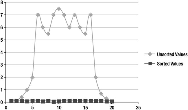
Figure 4-3. Storage index access times—sorted vs. unsorted
As you can see, sorted data will provide better and more consistent results. While we are on the subject, I should point out that there are many cases where several columns will benefit from this behavioral characteristic of storage indexes. It is common in data warehouse environments to have data that is partitioned on a date column, and there are often many other columns that track the partition key such as associated dates (order date, ship date, insert date, return date for example) or sequentially generated numbers like order numbers. Queries against these column are often problematic due the fact that partition eliminate cannot help them. Storage indexes will provide a similar benefit to partition elimination as long as care is taken to ensure that the data is pre-sorted prior to loading. This means sorting of table or partition data should be considered as part of moving or loading of data to increase efficiency of not only storage indexes, but Hybrid Columnar Compression, too. However, a given table or partition can only be sorted and stored on one column.
There’s no such thing as a free puppy. As with everything in life, there are a few issues with storage indexes that you should be aware of.
Incorrect Results
By far, the biggest issue with storage indexes has been that in early releases of the Exadata Storage Software, there were a handful of bugs regarding incorrect results. That is to say that in certain situations, usage of storage indexes could eliminate storage regions from consideration that actually contained records of interest. This incorrect elimination could occur due to timing issues with concurrent DML while a Smart Scan was being done using storage indexes. These bugs have been addressed in 11.2.0.2 and the patches on the storage servers of that time. At current times (Oracle 11.2.0.4/12.1.0.2), the chances of incorrect results are highly unlikely, which means not higher than would occur in other parts of the Oracle database. If you run into this issue or suspect you are running in this issue, disabling storage index usage via the hidden parameter, _KCFIS_STORAGEIDX_DISABLED by setting it to TRUE may be an option to diagnose differences in query results. If queries actually do produce different results with storage indexes, you can use this parameter to disable the usage of storage indexes either by setting it systemwide or by setting it for sessions until the proper patches are applied. This parameter can be set with an alter session command so that only problematic queries are affected. Of course, you should check with Oracle Support before enabling any hidden parameters. Also MOS note 1260804.1 (How to diagnose Smart Scan and wrong results) can be of help diagnosing potential Exadata/Smart-Scan-related issues, including storage indexes returning incorrect results.
Moving Target
Storage indexes can be a little frustrating because they do not always kick in when you expect them to. And because you cannot tell Oracle that you really want a storage index to exist and be used, there is little you can do other than try to understand why they are not there or used in certain circumstances so you can avoid those conditions in the future.
In early versions of the storage server software, one of the main reasons that storage indexes were disabled was due to implicit data type conversions. Over the years, Oracle has gotten better and better at doing “smart” data type conversions that do not have negative performance consequences. For example, if you write a SQL statement with a WHERE clause that compares a date field to a character string, Oracle will usually apply a to_date function to the character string instead of modifying the date column (which could have the unpleasant side effect of disabling an index). Unfortunately, when the Exadata storage software was relatively new, all the nuances had not been worked out, at least to the degree we’re used to from the database side. Dates have been particularly persnickety. Here is an example using cellsrv 11.2.1.2.6:
SYS@EXDB1> select count(*) from kso.skew3 where col3 = '20-OCT-05';

  COUNT(*)
----------
         0

Elapsed: 00:00:14.00
SYS@EXDB1> select name, value
  2  from v$mystat s, v$statname n
  3  where s.statistic# = n.statistic#
  4  and name like '%storage index%';

NAME                                                    VALUE
--------------------------------------------- ---------------
cell physical IO bytes saved by storage index               0

Elapsed: 00:00:00.01

SYS@EXDB1> select count(*) from kso.skew3 where col3 = '20-OCT-2005';

  COUNT(*)
----------
         0

Elapsed: 00:00:00.07

SYS@EXDB1> select name, value
  2  from v$mystat s, v$statname n
  3  where s.statistic# = n.statistic#
  4  and name like '%storage index%';

NAME                                                    VALUE
--------------------------------------------- ---------------
cell physical IO bytes saved by storage index     15954337792

Elapsed: 00:00:00.01
In this very simple example, there is a query with a predicate comparing a date column (col3) to a string containing a date. In one case, the string contained a four-digit year. In the other, only two digits were used. Only the query with the four-digit-year format used the storage index. Let’s look at the plans for the statements to see why the two queries were treated differently:
SYS@EXDB1> @fsx2
Enter value for sql_text: select count(*) from kso.skew3 where col3 = %
Enter value for sql_id:
Enter value for inst_id:

SQL_ID            AVG_ETIME  PX OFFLOAD IO_SAVED% SQL_TEXT
------------- ------------- --- ------- --------- ----------------------------------------
2s58n6d3mzkmn           .07   0 Yes        100.00 select count(*) from kso.skew3 where
                                                  col3 = '20-OCT-2005'

fuhmg9hqdbd84         14.00   0 Yes         99.99 select count(*) from kso.skew3 where
                                                  col3 = '20-OCT-05'

2 rows selected.

SYS@EXDB1> select * from table(dbms_xplan.display_cursor('&sql_id','&child_no','typical'));
Enter value for sql_id: fuhmg9hqdbd84
Enter value for child_no:

PLAN_TABLE_OUTPUT
--------------------------------------------------------------------------------------------
SQL_ID  fuhmg9hqdbd84, child number 0
-------------------------------------
select count(*) from kso.skew3 where col3 = '20-OCT-05'

Plan hash value: 2684249835

-------------------------------------------------------------------------
| Id|Operation                  |Name  | Rows|Bytes|Cost (%CPU)|Time    |
-------------------------------------------------------------------------
|  0|SELECT STATEMENT           |      |     |     |  535K(100)|        |
|  1| SORT AGGREGATE            |      |    1|   8 |           |        |
|* 2|  TABLE ACCESS STORAGE FULL|SKEW3 |  384|3072 |  535K  (2)|01:47:04|
-------------------------------------------------------------------------

Predicate Information (identified by operation id):
---------------------------------------------------

   2 - storage("COL3"='20-OCT-05')
       filter("COL3"='20-OCT-05')

20 rows selected.

SYS@EXDB1> /
Enter value for sql_id: 2s58n6d3mzkmn
Enter value for child_no:

PLAN_TABLE_OUTPUT
--------------------------------------------------------------------------------------------
SQL_ID  2s58n6d3mzkmn, child number 0
-------------------------------------
select count(*) from kso.skew3 where col3 = '20-OCT-2005'

Plan hash value: 2684249835

------------------------------------------------------------------------------------
| Id  | Operation                  | Name  | Rows  | Bytes | Cost (%CPU)| Time     |
------------------------------------------------------------------------------------
|   0 | SELECT STATEMENT           |       |       |       |   531K(100)|          |
|   1 |  SORT AGGREGATE            |       |     1 |     8 |            |          |
|*  2 |   TABLE ACCESS STORAGE FULL| SKEW3 |   384 |  3072 |   531K  (1)| 01:46:24 |
------------------------------------------------------------------------------------

Predicate Information (identified by operation id):
---------------------------------------------------

   2 - storage("COL3"=TO_DATE(' 2005-10-20 00:00:00', 'syyyy-mm-dd
              hh24:mi:ss'))
       filter("COL3"=TO_DATE(' 2005-10-20 00:00:00', 'syyyy-mm-dd
              hh24:mi:ss'))

22 rows selected.
It appears that the optimizer did not recognize the two-digit date as a date. At the very least, the optimizer failed to apply the to_date function to the literal, so the storage index was not used. Fortunately, most of these types of data conversion issues have been resolved with the later releases. Here is the same test using cellsrv 11.2.2.2.0:
SYS@SANDBOX> @si

NAME                                                                             VALUE
---------------------------------------------------------------------- ---------------
cell physical IO bytes saved by storage index                                        0

SYS@SANDBOX> select count(*) from kso.skew3 where col3 = '20-OCT-05';

  COUNT(*)
----------
         0

SYS@SANDBOX> @si

NAME                                                                             VALUE
---------------------------------------------------------------------- ---------------
cell physical IO bytes saved by storage index                              16024526848
As you can see, this conversion issue has been resolved. So, why bring it up? Well, the point is that the behavior of storage indexes has undergone numerous changes as the product has matured. As a result, we have built a set of test cases that we use to verify behavior after each patch in our lab. Our test cases primarily verify comparison operators (=,<,like, IS NULL, and so on) and a few other special cases such as LOBs, compression, and encryption. Of course, it is always a good practice to test application behavior after any patching, but if you have specific cases where storage indexes are critical to your application, you may want take special care to test those parts of you application.
Partition Size
Storage indexes depend on Smart Scans, which depend on direct path reads. As we discussed in Chapter 2, Oracle will generally use serial direct path reads for large objects. However, when an object is partitioned, Oracle may fail to recognize that the object is “large” because Oracle looks at the size of each individual segment. This may result in some partitions not being read via the Smart Scan mechanism and thus disabling any storage indexes for that partition. When historical partitions are compressed, the problem becomes even more noticeable, as the reduced size of the compressed partitions will be even less likely to trigger the serial direct path reads. This issue can be worked around by not relying on the serial direct path read algorithm and, instead, specifying a degree of parallelism for the object or using a hint to force the desired behavior.
Incompatible Coding Techniques
Finally, there are some coding techniques that can disable storage indexes. Here is an example showing the effect of the trunc function on date columns:
KSO@dbm2> select count(*) from skew3 where trunc(col3) = '20-OCT-2005';

  COUNT(*)
----------
         0
1 row selected.

Elapsed: 00:00:05.36

KSO@dbm2> @expl

PLAN_TABLE_OUTPUT
-----------------------------------------------------------------------------------------------------------------------------------------------------------
SQL_ID  2mkcfrs28z393, child number 0
-------------------------------------
select count(*) from skew3 where trunc(col3) = '20-OCT-2005'

Plan hash value: 2684249835

------------------------------------------------------------------------------------
| Id  | Operation                  | Name  | Rows  | Bytes | Cost (%CPU)| Time     |
------------------------------------------------------------------------------------
|   0 | SELECT STATEMENT           |       |       |       |   995K(100)|          |
|   1 |  SORT AGGREGATE            |       |     1 |     8 |            |          |
|*  2 |   TABLE ACCESS STORAGE FULL| SKEW3 |  7167K|    54M|   995K  (3)| 00:00:39 |
------------------------------------------------------------------------------------

Predicate Information (identified by operation id):
---------------------------------------------------

   2 - storage(TRUNC(INTERNAL_FUNCTION("COL3"))=TO_DATE(' 2005-10-20
              00:00:00', 'syyyy-mm-dd hh24:mi:ss'))
       filter(TRUNC(INTERNAL_FUNCTION("COL3"))=TO_DATE(' 2005-10-20
              00:00:00', 'syyyy-mm-dd hh24:mi:ss'))

22 rows selected.
In this example, a function was applied to a date column, which, as you might expect, disables the storage index. The fact that applying a function to a column disables the storage index is not too surprising, but application of the trunc function is a commonly seen coding technique. Many dates have a time component, and many queries want data for a specific day. It is well known that truncating a date in this manner will disable normal B-tree index usage. In the past, that generally did not matter. Queries in many data warehouse environments were designed to do full scans anyway, so there was really no need to worry about disabling an index. Storage indexes change the game from this perspective and may force us to rethink some of our approaches. We will discuss this issue in more detail in Chapter 16.
Summary
Storage indexes are an optimization technique that is available when the database is able to utilize Smart Table Scans. They can provide dramatic performance improvements, although the caching of Smart-Scanned data in the Flash Cache with recent cell server versions make Smart Scan performance come closer to storage index optimized performance. They are especially effective with queries that access data via an alternate key that tracks the primary partition key.
How the data is physically stored is an important consideration and has a dramatic impact on the effectiveness of storage indexes. Care should be taken when migrating data to the Exadata platform to ensure that the data is clustered on disk in a manner that will allow storage indexes to be used effectively. It should also be considered that storage indexes are limited to eight columns and are created dependent on predicates of SQL causing Smart Scans, fully automatic.