
![]()
Hybrid Columnar Compression
Hybrid Columnar Compression, or (E)HCC for short, was, and probably still is, one of the most misunderstood features in Exadata. This has not really changed since the first edition of this book, which is why we place such an emphasis on it. HCC started out as an Exadata-only feature, but its use is now available to a more general audience. Anyone who wants to use HCC at the time of this writing will have to either use Exadata or the Oracle ZFS Storage Appliance. The Pillar Axiom series of storage arrays also support working with HCC compressed data natively, without having to decompress it first. Oracle’s most recent storage offering, the FS1 array, also features HCC on its data sheet. Offloading scans of HCC data remains the domain of the Exadata storage cells though.
This chapter has been divided into three major areas:
- An introduction to how Oracle stores data physically on disk
- The concepts behind HCC and their implementation
- Common use cases and automating data lifecycle management
In the first part of this chapter, you will read more about the way the Oracle database stores information in what is referred to as the “Row Major” format. It explains the structure of the Oracle database block and two of the available compression methods: BASIC and ADVANCED.
Understanding the anatomy of the Oracle block is important before moving on to the next part of the chapter, which introduces the “Column Major” format unique to HCC. And in case you wondered about the “hybrid” in HCC, we will explain this as well. We will then discuss how the data is actually stored on disk, and when and where compression and decompression will occur. We will also explain the impact of HCC compressed data on Smart Scans as opposed to traditional ways of performing I/O.
The final part of this chapter is dedicated to the new Automatic Data Optimization option that helps automating and enforcing data lifecycle management.
As you probably already know, Oracle stores data in a block structure. These blocks are typically 8k nowadays. You define the default block size during the database creation. It is very difficult if not impossible to change the default block size after the database is created. There is good reason to stay with the 8k block size in a database as Oracle appears to perform most of its regression testing against that block size. And, if you really need to, you can still create tablespaces with different—usually bigger—block sizes.
Where does the database block fit into the bigger picture? The block is the smallest physical storage unit in Oracle. Multiple blocks form an extent, and multiple extents make up a segment. Segments are objects you work with in the database such as tables, partitions, and subpartitions.
Simplistically speaking, the block consists of a header, the table directory, a row directory, row data, and free space. The row header starts at the top of the block and works its way down, while the row data starts at the bottom and works its way up. Figure 3-1 shows the various components of a standard Oracle block in its detail.

Figure 3-1. The standard Oracle block format (row-major storage)
Rows are stored in no specific order, but columns are generally stored in the order in which they were defined in that table. For each row in a block there will be a row header, followed by the column data for each column. Figure 3-2 shows how the pieces of a row are stored in a standard Oracle block. Note that it is called a row piece because, occasionally, a row’s data may be stored in more than one chunk. In this case, there will be a pointer to the next row piece. Chapter 11 will introduce the implications of this in great detail.

Figure 3-2. The standard Oracle row format (row-major storage)
Note that the row header may contain a pointer to another row piece. More on this will follow a little later, but for now, just be aware that there is a mechanism to point to another location. Also note that each column is preceded by a separate field, indicating the length of the column. Nothing is actually stored in the column value field for NULL values. The presence of a null column is indicated by a value of 0 in the column length field. Trailing NULL columns do not even store the column length fields, as the presence of a new row header indicates that there are no more columns with values in the current row.
PCTFREE is a key value associated with blocks; it controls how much space is used in a block when inserting data before it is considered full. Its purpose is to reserve some free space in each block for (future) updates. This is necessary to prevent row migration (moving rows to new blocks) that would be caused by lack of space in the row’s original block when a row increases in size. When rows are expected to be updated with values requiring more space, more space in form of a higher PCTFREE setting can be reserved by the database administrator. When rows are not expected to increase in size because of updates, values as low as 0 may be specified by PCTFREE. With compressed blocks, it is common to use very low values of PCTFREE because the goal is to minimize space usage and rows are generally not expected to be updated. Figure 3-3 shows how free space is reserved based on the value of PCTFREE.
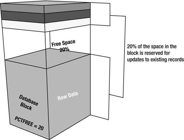
Figure 3-3. Block free space controlled by PCTFREE
Figure 3-3 shows a block that reserves 20 percent of its space for updates. A block with a PCTFREE setting of 0 percent would allow inserts to fill the block almost completely. When a record is updated and the new data will not fit in the available free space of the block where the record is stored, the database will move the row to a new block. This process is referred to as the said row migration. It does not completely remove the row from the original block but leaves a reference to the newly relocated row so that it can still be found by its original ROWID. The ROWID format defines how the database has to look up a row. It consists of the data object number, data file number, the data block, and finally the row in the block. The ROWID can be externalized by specifying the ROWID pseudo-column when querying a table. Oracle provides a package named DBMS_ROWID that allows you to parse the ROWID and extract the relevant bits of information you are after. The ROWID format will become important when you want to investigate the internals of a database block by dumping it into a trace file.
Note that the more generic term for storing rows in more than one piece is row chaining. Row migration is a special case of row chaining in which the entire row is relocated. Examples for row chaining and migration are presented in Chapter 11 of this book.
Disassembling the Oracle Block
So far you have only read about the concepts, but we intend to prove them as well, wherever possible. When you start looking at block dumps, then you can find all the cases of row chaining in the row headers. You can dump a block using the alter system dump datafile x block y syntax. Although the command is not documented officially, there are many sources that explain the technique. Here is an example of a small snippet from a block dump where the row is entirely contained in the same block. Most of the block dump information has been removed for clarity.
block_row_dump:
tab 0, row 0, @0x1f92
tl: 6 fb: --H-FL-- lb: 0x2  cc: 1
col  0: [ 2]  c1 02
tab 0, row 1, @0x1f8c
tl: 6 fb: --H-FL-- lb: 0x0  cc: 1
col  0: [ 2]  c1 03
The table definition has deliberately kept to the bare minimum, and there is just one column (named “ID”) of data type NUMBER in the table. The crucial information in this dump with regards to this discussion is the flag in the row header: According to David Litchfield’s article “The Oracle Database Block,” the flag byte (fb) in the row header can have the following bits set:
- K = Cluster Key
- C = Cluster table member
- H = Head piece of row
- D = Deleted row
- F = First data piece
- L = Last data piece
- P = First column continues from previous piece
- N = Last column continues in next piece
In the context of the block dump, the bits H, F, and L are set, translating to the head piece, first piece, and last piece. In other words, the column data that follows is sufficient to read the whole row. But how does Oracle know what to read in the block when it comes to row lookups? Oracle records in every block how many tables are to be found. Normally, you would only find one in there, but in some special cases such as BASIC/ADVANCED compressed blocks or clustered tables you can find two. The line starting “tab 0, row 0...” references the first table in the block, and row 0 is self-explanatory. The hexadecimal number following the @-sign is the offset within the block.
To better understand the importance of the offset, you need to look at the header structures preceding the row directory. The table-directory, which precedes the row directory in the block, lists the rows in the block and their location. Consulting the table directory together with the row directory allows Oracle to find the row in question and directly jump to the offset in the row directory shown above in the output from the block dump—one of the reasons why the lookup by ROWID is so efficient! The table directory (plus some detail from the data header) looks like this for the block dump shown above:
ntab=1
nrow=2
frre=-1
fsbo=0x16
fseo=0x1f8c
avsp=0x1f70
tosp=0x1f70
0xe:pti[0]      nrow=2  offs=0
0x12:pri[0]     offs=0x1f92
0x14:pri[1]     offs=0x1f8c
To locate the row, Oracle needs to find the offset to table 0 in the block and locate the row by means of the offset. In case of the first row, the offset is 0x1f92. This is found in the row data:
tab 0, row 0, @0x1f92
This explains why a table lookup by ROWID is so fast and efficient. Migrated rows, on the other hand, merely have the head piece set and none of the other flags. Here is an example from a different table:
block_row_dump:
tab 0, row 0, @0x1f77
tl: 9 fb: --H----- lb: 0x3  cc: 0
nrid:  0x00c813b6.0
tab 0, row 1, @0x1f6e
tl: 9 fb: --H----- lb: 0x3  cc: 0
nrid:  0x00c813b6.1
If you look carefully at the dump, you notice an additional piece of information. These rows have a NRID or next ROWID. This is the said pointer to the block where the row continues. A NRID pointer exists for all chained rows, including migrated rows. To decode the NRID, you can use the DBMS_UTILITY package. Careful though—the NRID is encoded in a hexadecimal format and first needs to be converted to a decimal value. Also, there is a limitation, even in 12c, that it does not seem to work with big file tablespaces. The NRID format finishes with a “.x” where x is the row number. To locate the block for NRID 0x00c813b6.0, you could use this script (the table resides on a smallfile tablespace):
SQL> !cat nrid.sql
select
     dbms_utility.data_block_address_file(to_number('&1','xxxxxxxxxxxx')) file_no,
     dbms_utility.data_block_address_block(to_number('&1','xxxxxxxxxxxx')) block_no
from dual;

SQL> @nrid 00c813b6

   FILE_NO   BLOCK_NO
---------- ----------
         7     529334
So the row continues in data file 7, block 529334.
A row can start in one block and continue in another bock (or even blocks), a phenomenon known as chained row. An example is shown here. The row begins in the block with DBA (Data Block Address) 0x014000f3:
tab 0, row 0, @0x30
tl: 8016 fb: --H-F--N lb: 0x0  cc: 1
nrid:  0x014000f4.0
col  0: [8004]
You can the start of the row (Head piece and First piece) and an indication that the row continues (Next) elsewhere. The NRID points to a DBA of 0x014000f4 and continues in row 0.
tab 0, row 0, @0x1f
tl: 8033 fb: ------PN lb: 0x0  cc: 1
nrid:  0x014000f5.0
Here, you see that the row has a Previous piece and a Next one to follow in DBA 0x014000f5, again row 0. This is a severe case of a chained row because it spans more than just two blocks. A few more row pieces later, we find the last remaining piece:
tab 0, row 0, @0x1d7c
tl: 516 fb: -----LP- lb: 0x0  cc: 1
The L in the flag byte indicates that this is the Last piece; the P flag indicates there are Previous row pieces. Coincidentally, this is how a HCC super-block, a so-called Compression Unit (CU), is constructed. In the previous example, a row was “spread” over a number of blocks, which is usually undesirable in row-major format. With HCC using the column-major format, however, you will see that this is a very clever design and not at all harmful for performance. You can read more about those Compression Units later, but first let’s focus on the available compression mechanics before the advent of HCC.
HCC is a relatively new compression technology in Oracle. Before its introduction, you had different compression mechanisms available at your disposal. The naming of the technologies has changed over time, and it is admittedly somewhat confusing. The syntax for using them also seems to change with every release. To keep a common denominator, the names BASIC, OLTP, and HCC will be used.
BASIC Compression
As the name suggests, BASIC compression is a standard feature in Oracle. To benefit from BASIC compression, you have to use the direct path method of injecting rows into the table. A direct path load basically bypasses the SQL engine and the transactional mechanism built into Oracle and inserts blocks above the segment’s high water mark or into an alternative “temporary” segment. More specifically, during the direct path insert, the buffer cache is not being utilized. After the direct path load operation finishes, it is mandatory to commit the transaction before anyone else can apply DML to the table. This is a concession to the faster loading process:
SQL> insert /*+ append */ into destination select * from dba_objects;

20543 rows created.

SQL> select * from destination;
select * from destination
              *
ERROR at line 1:
ORA-12838: cannot read/modify an object after modifying it in parallel
This is a major hindrance for using BASIC compression for anything but archival. Another “problem” is that updates to the data cause the updated row(s) to be stored uncompressed. The same is true for inserts not using the direct path loading mechanism.
Rows have always been stored in the format just shown in Oracle until HCC has been released—in so-called row-major format. The opposite of row-major format is the new HCC-specific column-major format you can read about later in this chapter. All BASIC compressed data will be stored self-contained within Oracle blocks. If you want to create a table with BASIC compression enabled, you can do so when you create the table or afterward:
SQL> create table T ... compress;

SQL> alter table T compress;
Note that changing a table from non-compressed to compress will not compress the data already stored in in. You first have to “move” the table, which causes the compaction of data. The command to move the table does not require the specification of a tablespace, allowing you to keep the table where it is. BASIC compression has been introduced in Oracle 9i. This form of compression is also known as Decision Support System (DSS) Compression. In fact, the term compression is slightly misleading. BASIC compression (and OLTP compression, for that matter) uses a de-duplication approach to reducing the amount of data to store. The details about this compression algorithm will be discussed in the next section.
OLTP Compression
OLTP compression has been one of the innovative features presented with Oracle 11g Release 1, but, unlike BASIC compression, its use requires you to have the license for the Advanced Compression Option. The Advanced Compression Option is not limited to database block compression, it can do more. An Oracle white paper describes all the use cases, and you will come across it again later in this chapter. Although the feature has been renamed to Advanced Row Compression in Oracle 12c we decided to go with its former name since we have grown so accustomed to it.
Recall from the previous section on BASIC compression that you need to use direct path operations in order to benefit from any compression. This requirement made it very difficult to use compression for tables and partitions that were actively being subjected to DML operations. If you did not use direct path operations on these, then you would increase concurrency at the cost of not compressing. If you sacrificed concurrency for storage footprint, you had to change your code and commit immediately after touching the segment. Neither of the two options are a solution, especially not the last one. OLTP compression removed the pain. Using OLTP compression, you do not need to use direct path operations for inserts, yet you benefit from compression. And unlike BASIC compression, which does not leave room in the block for future updates by default (PCTREE is 0), OLTP compression does.
Conceptually you start inserting into a new block. The rows are not compressed initially. Only when a threshold is reached will the block be compressed. This should free up some space in the block, and the block might end up available for DML again. After more rows are inserted, the threshold is hit again, data is compressed, and so forth until the block is fully utilized and compressed.
The syntax for using OLTP compression has changed; here are examples for 11g Release 1 and 2, and 12c Release 1:
SQL> -- 11.1 syntax
SQL> create table T ... compress for all operations;
SQL> -- 11.2 syntax
SQL> create table T ... compress for OLTP;
SQL> -- 12.1 syntax
SQL> create table T ... row store compress ADVANCED;
The parser in 12c Release 1 is backward compatible, but you should take the effort and update your scripts to the new syntax as the old DDL statements are deprecated.
OLTP compression is very important even if you are primarily going to compress using HCC, as it is the fallback compression method for any updated rows that previously were stored in a HCC compressed segment. An update on HCC compressed data cannot be done in-place. Instead, the row is migrated to an OLTP compressed block that might not even get compressed because it is mostly empty initially.
From a technical point of view, BASIC and OLTP compression are identical. Oracle uses de-duplication, in that it replaces occurrences of identical data with a symbol. The symbol must be looked up when reading the table; that is why, technically speaking, you find two tables in an OLTP compressed block. The first table contains the symbol table, while the second table contains the “real” data. The block dump—again reduced to the minimum necessary—shows the following:
bdba: 0x01437a2b
...
ntab=2
nrow=320
...
        r0_9ir2=0x0
        mec_kdbh9ir2=0x1c
                      76543210
        shcf_kdbh9ir2=----------
                  76543210
        flag_9ir2=--R---OC      Archive compression: N
                fcls_9ir2[0]={ }
                perm_9ir2[18]={ 8 16 0 17 15 14 10 13 11 1 5 6 2 12 3 4 9 7 }
0x28:pti[0]     nrow=53 offs=0
0x2c:pti[1]     nrow=267        offs=53
block_row_dump:
tab 0, row 0, @0x1dd6
tl: 7 fb: --H-FL-- lb: 0x0  cc: 15
col  0: *NULL*
col  1: [ 5]  56 41 4c 49 44
col  2: [ 1]  4e
col  3: *NULL*
col  4: [ 4]  4e 4f 4e 45
col  5: [ 1]  4e
col  6: [ 1]  4e
col  7: [ 1]  59
col  8: [ 3]  53 59 53
col  9: *NULL*
col 10: [ 7]  78 71 07 11 16 3c 0a
col 11: [19]  32 30 31 33 2d 30 37 2d 31 37 3a 32 31 3a 35 39 3a 30 39
col 12: [ 2]  c1 05
col 13: [ 7]  78 71 07 11 16 3c 0a
col 14: [ 5]  49 4e 44 45 58
bindmp: 00 55 0f 0e 20 1d 23
...
tab 1, row 0, @0x1dae
tl: 14 fb: --H-FL-- lb: 0x0  cc: 18
col  0: *NULL*
col  1: [ 5]  56 41 4c 49 44
col  2: [ 1]  4e
col  3: *NULL*
col  4: [ 4]  4e 4f 4e 45
col  5: [ 1]  4e
col  6: [ 1]  4e
col  7: [ 1]  59
col  8: [ 3]  53 59 53
col  9: *NULL*
col 10: [ 7]  78 71 07 11 16 3c 09
col 11: [19]  32 30 31 33 2d 30 37 2d 31 37 3a 32 31 3a 35 39 3a 30 38
col 12: [ 2]  c1 02
col 13: [ 7]  78 71 07 11 16 3c 09
col 14: [ 5]  54 41 42 4c 45
col 15: [ 2]  c1 03
col 16: [ 5]  49 43 4f 4c 24
col 17: [ 2]  c1 15
bindmp: 2c 00 04 03 1c cd 49 43 4f 4c 24 ca c1 15...
Things to note in the above output are highlighted in bold typeface. First of all, you see that there are two tables with 320 rows in total in the block. The ROWIDs with pti[0] and pti[1] explain where the number of rows per table and the table offset are for each of the two. Table 0 is the symbol table, and it is referenced by the bindmp in the “real” table, table 1. The algorithm on how to use the bindmp to locate symbols in the symbol table is out of the scope of this discussion. If you want to learn more about mapping symbol table to data table and how to read the row data as Oracle does, please refer to the article series “Compression in Oracle” by Jonathan Lewis.
Hybrid Columnar Compression
Finally, after that much introduction, you have reached the main section of this chapter—Hybrid Columnar Compression. As stated before, the use of HCC requires you to either use Exadata or the Oracle ZFS Storage Appliance or either the Pillar Axiom or Oracle FS1 storage array. Remember from the chapter on Smart Scans (Chapter 2) that a tablespace must be entirely contained on an Exadata storage server to be eligible for offload processing.
While you can manipulate HCC compressed data outside Exadata with the previously mentioned storage systems, you cannot get Smart Scans on these devices. So if you are not using any of these aforementioned storage devices, then you are out of luck. Although RMAN would restore HCC compressed data happily, accessing it while compressed does not work and you have to decompress before use (space permitting). Importing HCC compressed tables is possible if you specify the TABLE_COMPRESSION_CLAUSE of the TRANSFORM parameter so as to set the table compression to NOCOMPRESS for example. However this is a 12c feature.
[oracle@enkdb03 ~]$ impdp ... transform=table_compression_clause:nocompress
On the other hand, this might require a lot of space.
What Does the “Hybrid” in “Hybrid Columnar Compression” Mean?
Most relational database systems store data in a row-oriented format. The discussion of the Oracle block illustrates that concept: The Oracle database block contains row(s). Each row has multiple columns, and Oracle accesses these columns by reading the row, locating the column, reading the value (if it exits), and displaying the value to the end user. The basic unit the Oracle database engine operates on is the row. Row lookups by ROWID—or index-based lookups—are very efficient for most general-purpose and OLTP query engines. On the other hand, if you just want a single column of a table and perhaps to perform an aggregation on all the column’s values in that table, you incur significant overhead. The “wider” your table is (in other words, the more columns it has), the greater the overhead if you want to retrieve and work on just a single one.
Columnar database engines operate on columns rather than rows, reducing the overhead just mentioned. Unlike a standard Oracle block of 8kb, a columnar database will most likely employ a larger block size of multiples of those 8k we know from the Oracle engine. It might also store values for the column co-located, potentially with lots of optimizations already included in the way it stores the column. This is likely to make columnar access very fast. Instead of having to read the whole row to extract just the value of a single column, the engine can iterate over a large-ish block and retrieve many values in multi-block operations. Columnar databases, therefore, are more geared toward analytic or read-mostly workloads. Columnar databases cannot excel in row lookups by design. In order to read a complete row, multiple large-ish blocks of storage have to be read for each column in the table. Therefore, columnar databases are not very good for the equivalent of (full-row) ROWID lookups usually seen in OLTP workloads.
Oracle Hybrid Columnar Compression combines advantages of columnar data organization in that it stores columns separately within a new storage type, the so-called Compression Unit or CU. But unlike pure columnar databases, it does not neglect the “table access by index ROWID” path to retrieve information. The CU is written contiguously to disk in form of multiple standard Oracle blocks. Information pertaining to a given row is within the same CU, allowing Oracle to blindly issue one or two read requests matching the size of the CU and be sure that the row information has been retrieved. As you will see later in the chapter, Exadata accesses HCC compressed data in one of two modes: block oriented or via Smart Scan.
Making Use of Hybrid Columnar Compression
HCC compression requires you to use direct path operations (again!) just as with BASIC compression. This might sound like a step back from what was possible with OLTP-compression, but in our experience it is not. There are further things worth knowing about HCC that you will read about in the next few paragraphs outlining why HCC needs to be used with a properly designed data lifecycle management policy in mind. Conventional inserts and updates cause records to be stored outside the HCC specific CU while deletes simply cause the CU header information to be updated. In case of updates, rows will migrate to new blocks flagged for OLTP compression. Any of these new blocks marked for OLTP compression are not necessarily compressed straight away. If they are not filled up to the internal threshold, then nothing will happen initially, inflating the segment size proportionally to the number of rows updated.
With HCC, you can choose from four different compression types, as shown in Table 3-1. Note that the expected compression ratios are very rough estimates and that the actual compression ratio for your data can deviate significantly from these numbers.
Table 3-1. HCC Compression Types
|
Compression Type |
Description |
Expected Compression Ratio |
|---|---|---|
|
Query Low |
HCC Level 1 uses algorithm 1. As of Oracle 12.1, this is the LZO (Lempel–Ziv–Oberhumer) compression algorithm. This level provides the lowest compression ratios but requires the least CPU for compression and decompression operations. This algorithm is optimized for maximizing speed (specifically for row-level access). Decompression is very fast with this algorithm. |
4x |
|
Query High |
HCC Level 2 uses the ZLIB (gzip) compression algorithm as of Oracle 12.1. |
6x |
|
Archive Low |
HCC Level 3 uses the same compression algorithm as Query High but at a higher compression level. Depending on the data, however, the compression ratios may not exceed those of Query High by significant amounts. |
7x |
|
Archive High |
HCC Level 4 compression uses the Bzip2 compression algorithm as of 12.1. This is the highest level of compression available but is far and away the most CPU intensive. Compression times are often several times slower than for level 2 and 3. But again, depending on the data, the compression ratio may not be much higher than with Archive Low. This level is for situations where the regulator requires you to keep the data online while otherwise you would have archived it off to tertiary storage. Data compressed with this algorithm is truly cold and rarely touched. |
12x |
COMPRESSION ALGORITHMS
The implementation details of the various compression algorithms listed in Table 3-1 are current only at the time of this writing. Oracle reserves the right to make changes to the algorithm and refers to them in generic terms. The actual implementation is of little significance to the administrator since there is no control over them anyway. What remains a fact is that the higher the compression level, the more aggressive the algorithm. Aggressive in this context refers to how effective the data volume can be shrunk, and aggressiveness is directly proportional to CPU required. You can read more about the actual mechanics of compressing data later in the chapter.
The reference to the compression algorithms (LZO, GZIP, BZIP2) are all inferred from the function names in the Oracle code. The ORADEBUG utility helped printing short stack traces of the session compressing the data. As an example, here is the short stack for a create table statement for ARCHIVE HIGH compression:
BZ2_bzCompress()+144<-kgccbzip2pseudodo()+136<-kgccdo()+51<-kdzc_comp_buffer()+371<-kdzc_comp_colgrp()+595<-kdzc_comp_unit()+1598<-kdzc_comp_full_unit()+80<-kdzcompress()
Interestingly, but on the other hand not surprisingly, the code has changed from the first edition of the book. If you find references to functions beginning with kdz, there is a high probability they are used for HCC.
You can enable HCC when you create the table or partition, or afterward. Here are some code examples:
SQL> create table t_ql ... column store compress for query low;

SQL> create table t_ah ... column store compress for archive high;

SQL> alter table t1 modify partition p_jun_2013 column store compress for query high;
As with all previous examples, please note that changing a table or partition’s compression status using the alter table statement does not have any effect for data already stored in the segment. It applies for future (direct path) inserts only. To compress data already stored in the segment, you have to move the segment. The alter table . . . move statement does not require you to specify a destination tablespace. To query the dictionary about the current status of the segment compression, use COMPRESSION and COMPRESS_FOR columns found in DBA_TABLES, DBA_TAB_PARTITIONS, and DBA_TAB_SUBPARTITIONS, for example:
SQL> select table_name,compression,compress_for
  2  from user_tables;

TABLE_NAME                     COMPRESS COMPRESS_FOR
------------------------------ -------- ------------
T1                             DISABLED
T1_QL                          ENABLED  QUERY LOW
T1_QH                          ENABLED  QUERY HIGH
T1_AL                          ENABLED  ARCHIVE LOW
T1_AH                          ENABLED  ARCHIVE HIGH
But again, these do not reflect the actual size of the segment, or if the segment is actually compressed with that particular compression type. The impact of compression on table sizes is demonstrated using the tables above: T1 is uncompressed and serves as a baseline while the others are compressed with the different algorithms available in Oracle 12.1:
SQL> select s.segment_name, s.bytes/power(1024,2) mb, s.blocks,
  2  t.compression, t.compress_for, num_rows
  3  from user_segments s, user_tables t
  4  where s.segment_name = t.table_name
  5  and s.segment_name like 'T1%'
  6  order by mb;

SEGMENT_NAME                 MB     BLOCKS COMPRESS COMPRESS_FOR                    NUM_ROWS
-------------------- ---------- ---------- -------- ------------------------------ ---------
T1                         3840     491520 DISABLED                                 33554432
T1_QL                       936     119808 ENABLED  QUERY LOW                       33554432
T1_QH                       408      52224 ENABLED  QUERY HIGH                      33554432
T1_AL                       408      52224 ENABLED  ARCHIVE LOW                     33554432
T1_AH                       304      38912 ENABLED  ARCHIVE HIGH                    33554432
The compressed tables have been created using a CTAS statement on the same tablespace as the baseline table with exactly the same number of rows. Again, the compression ratios are for illustration only. Your data compression ratios are most likely different.
To find out more about the compression algorithm employed for a given row, you can use the built-in package DBMS_COMPRESSION. It features the GET_COMPRESSION_TYPE function that takes the owner, table name, and ROWID as arguments.
SQL> select id, rowid,
  2  dbms_compression.get_compression_type(user, 'T1_QL', rowid) compType
  3  from t1_ql where rownum < 3;

        ID ROWID                COMPTYPE
---------- ------------------ ----------
         1 AAAPAgAAKAAJogDAAA          8
         2 AAAPAgAAKAAJogDAAB          8
The meaning of these values is explained in the PL/SQL Packages and Types reference for the DBMS_COMPRESSION package. The compression type “8” indicates the use of the Query Low compression algorithm. If you now think you could run a running count(*) against the query to get the compression type of each block, you are mistaken—this takes far too long to be practical, even for “small” tables.
HCC Internals
The fact that data stored in the HCC format is stored in a new format—column major—has already been touched in the introduction to HCC compression. You could also read something about the way the HCC compressed data is stored internally. In this section, you can read more about the actual HCC mechanics.
First of all, the compressed data is stored in an Oracle meta-block, called a Compression Unit. This is the first and probably most visible of the innovative HCC features. It does not mean Oracle blocks as we know them are not used, just slightly differently.
Before going into more detail, I would like to present you with a symbolic block dump of a CU from Oracle 11.2.0.4, edited for brevity.
Block header dump:  0x014000f3
 Object id on Block? Y
 seg/obj: 0x420f  csc: 0x00.1bec83  itc: 3  flg: E  typ: 1 - DATA
...
bdba: 0x014000f3
data_block_dump,data header at 0x7f190a39b07c
=============================================
...
ntab=1
nrow=1
frre=-1
...
tosp=0x14
        r0_9ir2=0x0
        mec_kdbh9ir2=0x0
                      76543210
        shcf_kdbh9ir2=----------
                  76543210
        flag_9ir2=--R-----      Archive compression: Y
                fcls_9ir2[0]={ }
0x16:pti[0]     nrow=1  offs=0
0x1a:pri[0]     offs=0x30
block_row_dump:
tab 0, row 0, @0x30
tl: 8016 fb: --H-F--N lb: 0x0  cc: 1
nrid:  0x014000f4.0
col  0: [8004]
Compression level: 01 (Query Low)
 Length of CU row: 8004
kdzhrh: ------PC CBLK: 4 Start Slot: 00
 NUMP: 04
 PNUM: 00 POFF: 7954 PRID: 0x014000f4.0
 PNUM: 01 POFF: 15970 PRID: 0x014000f5.0
 PNUM: 02 POFF: 23986 PRID: 0x014000f6.0
 PNUM: 03 POFF: 32002 PRID: 0x014000f7.0
CU header:
CU version: 0   CU magic number: 0x4b445a30
CU checksum: 0xf47f1618
CU total length: 32502
CU flags: NC-U-CRD-OP
ncols: 6
nrows: 2459
algo: 0
CU decomp length: 32148   len/value length: 324421
row pieces per row: 1
num deleted rows: 0
START_CU:
 00 00 1f 44 0f 04 00 00 00 04 00 00 1f 12 01 40 00 f4 00 00 00 00 3e 62 01
 ...
This is not the entire CU, just the Head piece. The block dump for a CU looks like a block dump for a compressed Oracle block. Technically speaking, a CU is a chained row across a number of standard Oracle blocks written to disk contiguously. Every block stores one table and that table has just one row (ntab=1 and nrow=1). Even stranger, that one row just has a single column (cc: 1), even though the table DDL shows many more. The CU header identifies the block to be the CU’s head piece (Head, First, Next flags are set). The header describes the compressed data in the CU, such as the total length, number of columns, number of rows, the decompressed length, and the number of deleted rows. The actual data starts within the START_CU tag. A lot further down you will see an END_CPU and BINDMP. The Head piece of the CU also stores information about where the actual columns are located. A bitmap is encoded within the first block’s START_CU piece, indicating rows that have been deleted and pointers to where columns start. The row starting with NUMP lists the number of blocks in the CU. This CU uses Query Low as the compression algorithm, and it consists of four pieces located in blocks 0x014000f4, ...f5, ...f6, and ...f7 (= contiguously written to disk).
Conceptually, you can think about a CU as a logical concept similar to the one in Figure 3-4.

Figure 3-4. Schematic display of a Compression Unit
Each block is chained to the next one using the NRID notation and the “next” bit set in the row header. This is the second block of the CU. Note how the DBA is the next block adjacent to the Head piece.
block_row_dump:
tab 0, row 0, @0x1f
tl: 8033 fb: ------PN lb: 0x0  cc: 1
nrid:  0x014000f5.0
col  0: [8021]
Compression level: 01 (Query Low)
Also note how each block describes the data stored in it. In this case, it is Query Low. A self-describing block allows the user to change the compression algorithm ad libitum and still gives Oracle enough information on how to decompress the block. This is why DBMS_COMPRESSION.GET_COMPRESION_TYPE is so useful. What you can also derive from Figure 3-4 is that the rows are no longer stored together in the same way as before in row-major format. Instead, all the data is organized by column within the CU. The bitmap in the first block of the CU, contained between START_CU and END_CU tells Oracle where to find the column and the row within it. The way the CU is laid out is not what you would find in a pure columnar database, but rather a cross (“hybrid”) between the two. Remember that sorting is done only within a single CU, except for Query Low where sorting is not applied at load time to speed the process up. The next CU will start over with more data from column 1 again. The advantage of this format is that it allows a row to be read in its entirety by reading just a single CU. A pure columnar database would have to read multiple blocks, one for each column in the row. This is why Oracle can safely claim that index-based lookups to CUs are possible without the same overhead as for a pure columnar database. The disadvantage is that reading an individual record will require reading a multi-block CU instead of a single block. Of course, full table scans will not suffer because all the blocks will be read anyway. On the contrary, the full scan is most likely to benefit from the columnar storage format if your query references only the columns it actually needs. This way the code can loop through each CU in an efficient code-path referencing only columns required.
You will read more about the trade-offs a little later, but you should already be thinking that having to read the whole CU instead of just a block can be disadvantageous for tables that need to support lots of single row access. And remember that the CU is also compressed, which requires CPU cycles when decompressing it.
The sorting by columns is actually done to improve the effectiveness of the compression algorithms, not to get performance benefits of column-oriented storage. This is another contribution to the “hybrid” in HCC.
What Happens When You Create a HCC Compressed Table?
Tracing and instrumentation for HCC is embedded in the ADVCMP component. Using the new Universal Tracing Facility (UTS) for tracing Oracle, you can actually see what is happening when you are compressing a table. The syntax to enable UTS tracing for HCC is documented in ORADEBUG. Invoking ORADEBUG allows you to view what can be traced:
SQL> oradebug doc component ADVCMP

Components in library ADVCMP:
--------------------------------------------------------------------------
ADVCMP_MAIN           Archive Compression (kdz)
ADVCMP_COMP           Archive Compression: Compression (kdzc, kdzh, kdza)
ADVCMP_DECOMP         Archive Compression: Decompression (kdzd, kdzs)
ADVCMP_DECOMP_HPK     Archive Compression: HPK (kdzk)
ADVCMP_DECOMP_PCODE   Archive Compression: Pcode (kdp)
Although this component is documented even in 11g Release 2, the examples in this chapter are from 12.1.0.2. Interestingly, the ORADEBUG doc component command without arguments shows you code locations! From the previous code, you can derive that the KDZ* routines in Oracle seem to relate to HCC. This helps when viewing the trace file. Consider the following statement to enable tracing the compression (Warning: this can generate many gigabytes worth of trace data—do not ever run this in production, only in a dedicated lab environment. You risk filling up /u01 and causing huge problems otherwise):
SQL> alter session set events 'trace[ADVCMP_MAIN.*] disk=high';
If you are curious about the UTS syntax, just run oradebug doc event as described by co-author Tanel Poder on his blog. With the trace enabled, you can start compressing. Either use alter table ... move or create table ... column store compress for ... syntax to begin the operation and trace.
alter session set tracefile_identifier = 't2ql';
alter session set events 'trace[ADVCMP_MAIN.*] disk=high';

create table t2_ql
column store compress for query low
as select * from t2;

alter session set events 'trace[ADVCMP_MAIN.*] off';
![]() Note Be warned that the trace is very, very verbose, and it easily generates many GB worth of trace data, filling up your database software mount point and thus causing all databases to grind to a halt! Again, never run such a trace outside a dedicated lab environment.
Note Be warned that the trace is very, very verbose, and it easily generates many GB worth of trace data, filling up your database software mount point and thus causing all databases to grind to a halt! Again, never run such a trace outside a dedicated lab environment.
Before Oracle actually starts compressing, it analyzes the incoming data to work out the best way to compress the column. The trace will emit lines like these:
kdzcinit(): ctx: 0x7f9f4b7a1868  actx: (nil)  zca: (nil)  ulevel: 1  ncols: 8 totalcols: 8
kdzainit(): ctx: 7f9f4b7a2d48 ulevel 1 amt 1048576 row 4096 min 5
kdzalcd(): objn: 61487 ulevel: 1
kdzalcd(): topalgo: -1 err: 100
kdza_init_eq(): objn: 61487  ulevel: 1  enqueue state:0
kdzhDecideAlignment(): pnum: 0 min_target_size: 32000 max_target_size: 32000
  alignment_target_size: 128000 ksepec: 0 postallocmode: 0 hcc_flags: 0
kdzh_datasize(): freesz: 0 blkdtsz: 8168 flag: 1 initrans: 3 dbidl: 8050 dbhsz: 22
  dbhszz: 14 drhsz: 9 maxmult: 140737069841520
kdzh_datasize(): pnum: 0 ds: 8016 bs: 8192 ov: 20 alloc_num: 7 min_targetsz:
  32000 max_targetsz: 32000 maxunitsz: 40000 delvec_size: 7954
kdzhbirc(): pnum: 0 buffer 1 rows soff: 0
...
It appears as if the calls to KDZA* initialize the data analyzer for object 61487 (Table T2_QL). ULEVEL in the trace possibly relates to the compression algorithm 1 (Query Low, as you will see in the block dump). The output related to kdzh_datasize() looks related to the CU header and compression information. The next lines are concerned with filling a buffer and needed to get an idea about the data to be compressed. Once that first buffer has been filled, the analyzer creates a new CU. For higher compression levels, Oracle will try to pre-sort the data before compressing it. This may not make sense in all cases—if the analyzer detects such a case, it will skip the sorting for that column. Oracle can also perform column permutation if it adds a benefit to the overall compression.
The result of this operation is presented in the analyzer context:
Compression Analyzer Context Dump Begin
---------------------------------------
ctx: 0x7f9f4b7a2d48  objn: 61487
Number of columns: 8
ulevel: 1
ilevel: 4645
Top algorithm: 0
Sort column: None
Total Output Size: 109435
Total Input Size: 396668
Grouping: Column-major, columns separate

Column Permutation Information
------------------------------
Columns not permuted
Total Number of rows/values  : 4096

Column Information
------------------
Col     Algo    InBytes/Row      OutBytes/Row    Ratio   Type    Name     Type Name
---     ----    -----------      ------------    -----   ----    ----     ---------
0       1025            4.0              3.01      1.3   2       NULL     NUMBER
1       257            11.0              4.11      2.7   1       NULL     CHAR
2       1025            4.0              3.01      1.3   2       NULL     NUMBER
3       1025            3.0              0.05     60.5   2       NULL     NUMBER
4       1025            5.0              4.08      1.2   2       NULL     NUMBER
5       1025            4.9              4.01      1.2   2       NULL     NUMBER
6       257             4.0              3.07      1.3   2       NULL     NUMBER
7       257            61.0              5.41     11.3   1       NULL     CHAR

Total                                    96.8         26.75       3.6

Column Metrics Information
--------------------------
Col     Unique  Repeat   AvgRun  DUnique DRepeat AvgDRun
---     ------  ------   ------  ------- ------- -------
0         4096       0      1.0        0       0     0.0
1         4096       0      1.0        0       0     0.0
2         4096       0      1.0        0       0     0.0
3           47      46     95.3        0       0     0.0
4         4082      14      1.0        0       0     0.0
5         4061      35      1.0        0       0     0.0
6         3646     408      1.0        0       0     0.0
7         3841     241      1.0        0       0     0.0

Compression Analyzer Context Dump End
-------------------------------------
The result of the analysis is then stored in the dictionary for reuse.
![]() Note This step is not needed when the analysis has already been performed, such as when inserting into a HCC compressed segment.
Note This step is not needed when the analysis has already been performed, such as when inserting into a HCC compressed segment.
Unfortunately, there does not seem to be an easy way to extract the analyzer information once it has been stored. Before writing the CU, you can see lots of interesting information about it in kdzhailseb() before the CUs are dumped for the table. The functions referenced in the trace file are also easily visible in the ORADEBUG short stack. The traces also helped confirm the various CU sizes Oracle tries to create, as found in kdzhDecideAlignment(). Table 3-2 lists the result of different create table statement for all four compression algorithms.
Table 3-2. Target CU Sizes and Their Alignment Target for Oracle 12.1.0.2
|
Compression Type |
min_target_size |
max_target_size |
|---|---|---|
|
Query Low |
32000 |
32000 |
|
Query High |
32000 |
64768 |
|
Archive Low |
32000 |
261376 |
|
Archive High |
261376 |
261376 |
Remember that the same algorithm (GZIP when this text was written) is used for Query High and Archive Low. Another observation we made is that the actual CU size can vary, except for Archive High where it appears fixed.
HCC Performance
There are three areas of concern when discussing performance related to table compression. The first is load performance. It addresses the question how long it takes to load the data. Since compression always happens on the compute nodes and during direct path operations, it is essential to measure the impact of compression on loads. The second area of concern, query performance, is the impact of decompression and other side effects on queries against the compressed data. The third area of concern, DML performance, is the impact compression algorithms have on other DML activities such as updates and deletes.
As you might expect, load time tends to increase with the amount of compression applied. As the saying goes, “There is no such thing as a free lunch.” Compression is computationally expensive—there is no doubt about that. The more aggressive the compression algorithm, the more CPU cycles you are going to use. The algorithms Oracle currently implements range from LZO to GZIP and BZIP2, with LZO yielding the lowest compression ratio but shortest compression time. BZIP2 can potentially give you the best compression but at the cost of huge CPU usage. There is an argument that states that data compressed with ARCHIVE HIGH is better decompressed to ARCHIVE LOW before querying it repeatedly. Compression ratios are hugely dependent on data-a series of the character “c”, repeated a billion times can be represented with very little that is already compressed such as a JPEG image cannot be compressed further.
With this introduction, it is time to look at an example. The data in the table T3 is reasonably random. To increase the data volume, it has been copied over itself a number of times (insert into t3 select * from t3 for a total size of 11.523 GB). The table has then been subjected to compression using BASIC, OLTP, and all HCC compression algorithms. The outcome is reported in Table 3-3.
Table 3-3. The Effect of Compression on the Example. Table-Load Has Been Performed Serially
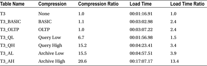
As you can see, Query High and Archive Low yield almost identical compression ratios for this particular data set. Loading the data took roughly 30 seconds more. Loading data with compression enabled definitely has an impact—the duration to create the table is somewhere between 2.5 and 4 times longer than without compression. What is interesting is that BASIC and OLTP compression almost make no difference at all in storage space used. Not every data set is equally well compressible. Timings here are taken from an X2 system; current Exadata systems have faster and more efficient CPUs.
The compression ratios increase by a few magnitudes as soon as HCC is enabled. The load times increase in line with the storage savings except for Archive High, which we will get back to later. Loading data serially, however, is rather pedestrian in Exadata, and significant performance gains can be made by parallelizing the load operation.
![]() Note You can read more about parallel operations in Chapter 6.
Note You can read more about parallel operations in Chapter 6.
Be warned that even though Exadata is a very powerful platform, you should not overload your system with parallel queries and parallel DML! And also note you do not have to insert into HCC compressed segments. Depending on your strategy you can introduce compression at later stages.
Load time is only the first performance metric of interest. Once the data is loaded, it needs to be accessible in reasonable time as well! Most systems load data once and read it many times more often. Query performance is a mixed bag when it comes to compression. Depending on the type of query, compression can either speed it up or slow it down. Decompression can add overhead in the way of additional CPU usage, especially if it has to be performed on the compute node. The offset of using more CPU to decompress the data is on disk access. Compressed data means fewer blocks need to be physically read from disk. If the query favors the column-major format of the HCC compressed rows, additional gains are possible. These combined usually outweigh the extra cost of decompressing.
There are essentially two access patterns with HCC compressed data: Smart Scan or traditional block I/O. The importance of these lies in the way that HCC data is decompressed. For non-Smart Scans, the decompression will have to be performed on the compute node. An interesting question in this context is how long it takes to retrieve a row by its ROWID. It seems logical that the larger the CU, the longer it takes to decompress it. You may have asked yourself the question in previous sections of this chapter where the difference was between Query High and Archive Low, apart obviously from the CU size. The gist of it is that Archive High gives you slightly better compression and offloaded full table scans. ROWID access, which often is not a Smart Scan, with Archive Low is inherently a little worse due to the larger CU size. As with so many architectural decisions, it comes down again to “knowing your data.”
Another important aspect is related to Lifecycle Management. Imagine a situation where the table partition in its native form is eligible for Smart Scans. Reports and any data access that relies on offloaded scans will perform at the expected speed. It is well possible that introducing compression to that partition over its lifetime will reduce the size to an extent where the segment is no longer eligible for Smart Scans. This may have a performance impact, but not necessarily so. We have seen many cases where the storage savings, in addition to the column-major format, more than outweighed the missing Smart Scans.
Returning to another set of demonstration tables that have been subject to compression, we would like to demonstrate the different types of I/O and their impact on query performance. The demonstration tables used in this section contain 128 million rows and have the following sizes:
SQL> select owner,segment_name,segment_type,bytes/power(1024,2) m, blocks
  2  from dba_segments
  3  where segment_name like 'T3%' and owner = 'MARTIN'
  4  order by m;

OWNER                SEGMENT_NAME                   SEGMENT_TYPE                M     BLOCKS
-------------------- ------------------------------ ------------------ ---------- ----------
MARTIN               T3_AH                          TABLE                    2240     286720
MARTIN               T3_QH                          TABLE                    3136     401408
MARTIN               T3_AL                          TABLE                    3136     401408
MARTIN               T3_QL                          TABLE                    6912     884736
MARTIN               T3_BASIC                       TABLE                   71488    9150464
MARTIN               T3_OLTP                        TABLE                   80064   10248192
MARTIN               T3                             TABLE                80100.75   10252896

8 rows selected.
In the first step, statistics are calculated on all of them using a call to DBMS_STATS as shown:
SQL> exec dbms_stats.gather_table_stats(ownname => user, tabname => 'T3', -
  2  method_opt=>'for all columns size 1', degree=>4)
The times per table are listed in Table 3-4.
Table 3-4. The Effect of Compression on the Gathering Statistics

Gathering statistics is certainly something that is more CPU intensive. The above examples were run with a very moderate Degree Of Parallelism (DOP) of 4. Increasing the DOP to 32 is suited to put quite a strain on the machine:
top - 02:41:02 up 95 days,  8:48,  5 users,  load average: 7.97, 3.34, 2.10
Tasks: 1357 total,  20 running, 1336 sleeping,   0 stopped,   1 zombie
Cpu(s): 85.8%us,  5.2%sy,  0.0%ni,  8.4%id,  0.0%wa,  0.0%hi,  0.6%si,  0.0%st
Mem:  98807256k total, 97729000k used,  1078256k free,   758456k buffers
Swap: 25165820k total,  5640088k used, 19525732k free, 13032976k cached

  PID USER      PR  NI  VIRT  RES  SHR S %CPU %MEM    TIME+  COMMAND
21209 oracle    20   0 8520m  19m  10m S 79.6  0.0   0:29.42 ora_p00k_db12c1
21239 oracle    20   0 8520m  19m  10m R 77.3  0.0   0:29.35 ora_p00r_db12c1
21247 oracle    20   0 8520m  20m  10m S 76.0  0.0   0:29.56 ora_p00v_db12c1
21110 oracle    20   0 8539m  35m  13m S 74.0  0.0  47:07.75 ora_p002_db12c1
21241 oracle    20   0 8520m  19m  10m R 73.7  0.0   0:28.33 ora_p00s_db12c1
21203 oracle    20   0 8520m  20m  10m S 73.4  0.0   0:29.35 ora_p00j_db12c1
21185 oracle    20   0 8520m  20m  10m R 71.7  0.0   0:28.86 ora_p00g_db12c1
21245 oracle    20   0 8520m  18m  10m R 71.1  0.0   0:28.66 ora_p00u_db12c1
21167 oracle    20   0 8532m  28m  11m R 69.4  0.0   3:46.38 ora_p00e_db12c1
21225 oracle    20   0 8520m  18m  10m R 69.4  0.0   0:28.43 ora_p00o_db12c1
21243 oracle    20   0 8520m  20m  10m S 69.1  0.0   0:29.29 ora_p00t_db12c1
21217 oracle    20   0 8520m  19m  10m S 68.8  0.0   0:29.68 ora_p00m_db12c1
As you can see, the compression slowed down the processing enough to outweigh the gains from the reduced number of data blocks that need to be read. This is due to the CPU intensive nature of the work being done.
Next up is another example that uses a very I/O intensive query. This test uses a query without a where clause that spends most of the time retrieving data from the storage layer via Smart Scans. First is the query against the baseline table—with a size of 80 GB. To negate the effect the automatic caching of data in Flash Cache has, this feature has been disabled on all tables. In addition, storage indexes have been disabled to ensure comparable results between the executions.
SQL> select  /*+ parallel(16) monitor gather_plan_statistics */
  2  /* hcctest_io_001 */
  3  sum(id) from t3;

   SUM(ID)
----------
1.0240E+15

Elapsed: 00:00:07.33
In Table 3-5, we compare this time to all the other tables.
Table 3-5. The Effect of Compression on Full-Table Scans

Automatic caching of data on Cell Flash Cache can contribute significantly to performance. Due to the fact that T3 was used as the basis for the creation of all other tables, large portions of it were found on flash cache. The initial execution time was 00:00:07.33. Cell Flash Cache as well as storage indexes were disabled when executing the queries whose runtime was recorded in Table 3-5. But since automatic caching of data is so beneficial for overall query performance, you should not disable Cell Flash Cache for a table. Leaving it at the default is usually sufficient from cell version 11.2.3.3.0 onward.
Executing these queries does not require a lot of CPU usage on the compute nodes. Since these operations were offloaded, only the cells were busy. The immense reduction in execution time is mostly due to the smaller size to be scanned. Although the Smart Scan is performed on the cells, they cannot skip reading data since storage indexes were disabled. The system had to go through roughly 80GB in the baseline and a mere 3 GB for Query High. Here is an example for the CPU usage during one of the queries:
top - 03:47:25 up 95 days,  9:54,  4 users,  load average: 2.23, 1.78, 1.84
Tasks: 1349 total,   5 running, 1343 sleeping,   0 stopped,   1 zombie
Cpu(s):  3.1%us,  1.3%sy,  0.0%ni, 95.5%id,  0.1%wa,  0.0%hi,  0.1%si,  0.0%st
Mem:  98807256k total, 95911576k used,  2895680k free,   356604k buffers
Swap: 25165820k total,  5731988k used, 19433832k free, 11756500k cached

  PID USER      PR  NI  VIRT  RES  SHR S %CPU %MEM    TIME+  COMMAND
21116 oracle    20   0 8551m  39m  13m R 55.6  0.0  15:14.08 ora_p005_db12c1
21153 oracle    20   0 8540m  28m  11m S 48.2  0.0   4:58.39 ora_p00c_db12c1
21108 oracle    20   0 8553m  45m  14m S 44.5  0.0  49:14.08 ora_p001_db12c1
21112 oracle    20   0 8548m  43m  13m S 44.5  0.0  47:26.76 ora_p003_db12c1
21136 oracle    20   0 8528m  28m  11m S 42.6  0.0   4:59.52 ora_p00a_db12c1
21110 oracle    20   0 8539m  35m  14m S 40.8  0.0  48:24.29 ora_p002_db12c1
21106 oracle    20   0 8539m  36m  14m S 38.9  0.0  49:21.38 ora_p000_db12c1
21122 oracle    20   0 8568m  39m  13m S 37.1  0.0  15:01.77 ora_p007_db12c1
21149 oracle    20   0 8536m  29m  11m R 37.1  0.0   4:58.12 ora_p00b_db12c1
21175 oracle    20   0 8528m  29m  11m S 37.1  0.0   5:01.79 ora_p00f_db12c1
21118 oracle    20   0 8544m  45m  13m R 35.2  0.0  14:57.77 ora_p006_db12c1
21161 oracle    20   0 8544m  30m  11m S 35.2  0.0   5:01.12 ora_p00d_db12c1
21114 oracle    20   0 8547m  42m  13m S 33.4  0.0  15:09.21 ora_p004_db12c1
21126 oracle    20   0 8544m  30m  11m S 33.4  0.0   4:55.96 ora_p008_db12c1
21130 oracle    20   0 8536m  28m  11m R 29.7  0.0   5:00.08 ora_p009_db12c1
21167 oracle    20   0 8528m  28m  11m S 27.8  0.0   5:04.26 ora_p00e_db12c1
22936 root      20   0 11880 2012  748 S 13.0  0.0   0:39.81 top
Generally speaking, records that will be updated should not be compressed. When you update a record in an HCC table, the record will be migrated to a new block that is flagged as an OLTP compressed block. Of course, a pointer will be left behind so that you can still get to the record via its old ROWID, but the record will be assigned a new ROWID as well. Since updated records are downgraded to OLTP compression, you need to understand how that compression mechanism works on updates. Figure 3-5 demonstrates how non-direct path loads into an OLTP block are processed.

Figure 3-5. The OLTP compression process for non-direct path loads
The progression of states moves from left to right. Rows are initially loaded in an uncompressed state. As the block fills to the point where no more rows can be inserted, the row data in the block is compressed. The block is then made available again and is capable of accepting more uncompressed rows. This means that in an OLTP compressed table, blocks can be in various states of compression. All rows can be compressed, some rows can be compressed, or no rows can be compressed. This is exactly how records in HCC blocks behave when they are updated. A couple of examples will demonstrate this behavior. The first example will show how the size of a table can balloon with updates. Before the update, the segment was 408 MB in size. The uncompressed table is listed here for comparison:
SQL> select segment_name,trunc(bytes/power(1024,2)) m
  2  from user_segments where segment_name in ('T1', 'T1_QH'),

SEGMENT_NAME                            M
------------------------------ ----------
T1                                   3840
T1_QH                                 408
Next, the entire compressed table is updated. After the update completes, you should check its size:
SQL> update t1_qh set id = id + 1;

33554432 rows updated.

SQL> select segment_name,trunc(bytes/power(1024,2)) m
  2  from user_segments where segment_name in ('T1','T1_QH')
  3  order by segment_name;

SEGMENT_NAME                                         M
-------------------------------------- ---------------
T1                                            3,841.00
T1_QH                                         5,123.00

2 rows selected.
At this point, you will notice that the updated blocks are of type 64-OLTP, compressed as a result of an update from a HCC compressed table. A call to DBMS_COMPRESSION.GET_COMPRESSION_TYPE confirms this:
SQL> select decode (dbms_compression.get_compression_type(user,'T1_QH',rowid),
  2     1,  'COMP_NOCOMPRESS',
  3     2,  'COMP_FOR_OLTP',
  4     4,  'COMP_FOR_QUERY_HIGH',
  5     8,  'COMP_FOR_QUERY_LOW',
  6     16, 'COMP_FOR_ARCHIVE_HIGH',
  7     32, 'COMP_FOR_ARCHIVE_LOW',
  8     64, 'COMP_BLOCK',
  9     'OTHER') type
 10  from T1_QH
 11* where rownum < 11
SQL> /

TYPE
---------------------
COMP_BLOCK
COMP_BLOCK
COMP_BLOCK
COMP_BLOCK
COMP_BLOCK
COMP_BLOCK
COMP_BLOCK
COMP_BLOCK
COMP_BLOCK
COMP_BLOCK

10 rows selected.
The above is an example for 11.2.0.4. The constraints in DBMS_COMPRESSION have been renamed in Oracle 12c—the “FOR” has been removed and COMP_FOR_OLTP is now known as COMP_ADVANCED. As soon as you re-compress the table, the size returns back to normal.
SQL> select segment_name,trunc(bytes/power(1024,2)) m
  2  from user_segments where segment_name in ('T1','T1_QH')
  3  order by segment_name;

SEGMENT_NAME                                         M
---------------------------------------- -------------
T1                                            3,841.00
T1_QH                                           546.00

2 rows selected.
The second example demonstrates what happens when you update a row. Unlike in previous versions of the software, the updated row is not migrated, as you will see. It is deleted from the CU, but there is no pointer left behind where the row migrated. This helps avoiding following the chained row visible in the “table fetch continued row” statistic.
Here is the table size with all rows compressed. The table needs to be on a SMALLFILE tablespace if you want to follow the example. The table does not need to contain useful information, it is merely big.
SQL> create table UPDTEST_QL column store compress for query low
  2  tablespace users as select * from UPDTEST_BASE;

Table created.

SQL> select segment_name, bytes/power(1024,2) m, compress_for
  2  from user_segments s left outer join user_tables t
  3  on (s.segment_name = t.table_name)
  4  where s.segment_name like 'UPDTEST%'
  5  /

SEGMENT_NAME                            M COMPRESS_FOR
------------------------------ ---------- ------------------------------
UPDTEST_QL                             18 QUERY LOW
UPDTEST_BASE                         1344
For the example, you need to get the first ID from the table and some other meta information:
SQL> select dbms_compression.get_compression_type(user,'UPDTEST_QL',rowid) as ctype,
  2  rowid, old_rowid(rowid) DBA, id from UPDTEST_QL where id between 1 and 10
  3  /

     CTYPE ROWID              DBA                          ID
---------- ------------------ -------------------- ----------
         8 AAAG6TAAFAALORzAAA 5.2942067.0                   1
         8 AAAG6TAAFAALORzAAB 5.2942067.1                   2
         8 AAAG6TAAFAALORzAAC 5.2942067.2                   3
         8 AAAG6TAAFAALORzAAD 5.2942067.3                   4
         8 AAAG6TAAFAALORzAAE 5.2942067.4                   5
         8 AAAG6TAAFAALORzAAF 5.2942067.5                   6
         8 AAAG6TAAFAALORzAAG 5.2942067.6                   7
         8 AAAG6TAAFAALORzAAH 5.2942067.7                   8
         8 AAAG6TAAFAALORzAAI 5.2942067.8                   9
         8 AAAG6TAAFAALORzAAJ 5.2942067.9                  10
The function old_rowid() is available from the Enkitec blog and the online code repository in file create_old_rowid.sql. It decodes the ROWID to get the Data Block Address or the location on disk. In the above example, ID 1 is in file 5, block 2942067, and slot 0. A compression type of 8 indicates Query Low. Let’s begin the modification:
SQL> update UPDTEST_QL set spcol = 'I AM UPDATED' where id between 1 and 10;

10 rows updated.

SQL> commit;

Commit complete.

SQL> select dbms_compression.get_compression_type(user,'UPDTEST_QL',rowid) as ctype,
  2  rowid, old_rowid(rowid) DBA, id from updtest_ql where id between 1 and 10;

     CTYPE ROWID              DBA                          ID
---------- ------------------ -------------------- ----------
        64 AAAG6TAAFAAK4jhAAA 5.2853089.0                   1
        64 AAAG6TAAFAAK4jhAAB 5.2853089.1                   2
        64 AAAG6TAAFAAK4jhAAC 5.2853089.2                   3
        64 AAAG6TAAFAAK4jhAAD 5.2853089.3                   4
        64 AAAG6TAAFAAK4jhAAE 5.2853089.4                   5
        64 AAAG6TAAFAAK4jhAAF 5.2853089.5                   6
        64 AAAG6TAAFAAK4jhAAG 5.2853089.6                   7
         1 AAAG6TAAFAAK4jkAAA 5.2853092.0                   8
         1 AAAG6TAAFAAK4jkAAB 5.2853092.1                   9
         1 AAAG6TAAFAAK4jkAAC 5.2853092.2                  10

10 rows selected
As you can see, the compression type of some of the updated rows has changed to 64, which is defined as COMP_BLOCK in DBMS_COMPRESSION. This particular type is indicated in cases where an updated block is moved out of its original CU and into an OLTP compressed block. Up to Oracle 11.2.0.2, you would see a compression type of 2 or COMP_ADVANCED/COMP_FOR_OLTP. How can you tell the block has moved? Compare the new Data Block Address with the original one: Instead of file 5 block 2942067 slot 0, the block containing ID 1 is now on file 5 block 2853089 slot 0.
The question now is what happened to the data if we queried the table with the original ROWID for ID 1:
SQL> select id,spcol from updtest_ql where rowid = 'AAAG6TAAFAALORzAAA';

no rows selected
This behavior is different from when we initially described the effect of an update. You can find the original reference at Kerry Osborne’s blog:
http://kerryosborne.oracle-guy.com/2011/01/ehcc-mechanics-proof-that-whole-cus-are-not-decompressed/
The old ROWID is not accessible anymore. What about the new one? You would really hope that worked:
SQL> select id,spcol from updtest_ql where rowid = 'AAAG6TAAFAAK4jhAAA';

        ID SPCOL
---------- ----------------------------------------
         1 I AM UPDATED
During the research for this updated edition, it was not possible to create a test case where a row has been truly migrated. In other words, it was not possible to retrieve an updated row using its old ROWID. This sounds odd at first but, on the other hand, simplifies processing. If Oracle left a pointer for the new row in place, it would have to perform another lookup on the new block, slowing down processing. If we dump the new block on file 5 block 2853089, you can see that it is indeed an OLTP compressed block. Note that the rows in the next block from the above listing are not compressed. A compression type of 1 translates to uncompressed.
SQL> alter system dump datafile 5 block 2853089;

System altered.

SQL> @trace
SQL> select value from v$diag_info where name like 'Default%';

VALUE
-------------------------------------------------------------------
/u01/app/oracle/diag/rdbms/dbm01/dbm011/trace/dbm011_ora_53134.trc

Block header dump:  0x016b88e1
 Object id on Block? Y
 seg/obj: 0x6e93  csc: 0x00.607114  itc: 2  flg: E  typ: 1 - DATA
     brn: 0  bdba: 0x16b8881 ver: 0x01 opc: 0
     inc: 0  exflg: 0

 Itl           Xid                  Uba         Flag  Lck        Scn/Fsc
0x01   0x002c.00d.00000007  0x0020d085.0017.02  --U-    7  fsc 0x0000.00607122
0x02   0x0000.000.00000000  0x00000000.0000.00  ----    0  fsc 0x0000.00000000
bdba: 0x016b88e1
data_block_dump,data header at 0x7f5c8fb6d464
===============
tsiz: 0x1f98
hsiz: 0x34
pbl: 0x7f5c8fb6d464
     76543210
flag=-0----X-
ntab=2
nrow=11
frre=-1
fsbo=0x34
fseo=0x372
avsp=0x33e
tosp=0x33e
        r0_9ir2=0x1
        mec_kdbh9ir2=0x0
                      76543210
        shcf_kdbh9ir2=----------
                  76543210
        flag_9ir2=--R-LN-C      Archive compression: N
                fcls_9ir2[0]={ }
0x16:pti[0]     nrow=4  offs=0
0x1a:pti[1]     nrow=7  offs=4
0x1e:pri[0]     offs=0x1f7e
...
block_row_dump:
tab 0, row 0, @0x1f7e
tl: 11 fb: --H-FL-- lb: 0x0  cc: 1
col  0: [ 8]  54 48 45 20 52 45 53 54
bindmp: 00 06 d0 54 48 45 20 52 45 53 54
...
tab 1, row 0, @0x1b6f
tl: 1019 fb: --H-FL-- lb: 0x1  cc: 6
col  0: [ 2]  c1 02
col  1: [999]
 31 20 20 20 20 20 20 20 20 20 20 20 20 20 20 20 20 20 20 20 20 20 20 20 20
 20 20 20 20 20 20 20 20 20 20 20 20 20 20 20 20 20 20 20 20 20 20 20 20 20
...
col  2: [ 7]  78 71 0b 16 01 01 01
col  3: [ 7]  78 71 0b 16 12 1a 39
col  4: [ 8]  54 48 45 20 52 45 53 54
col  5: [12]  49 20 41 4d 20 55 50 44 41 54 45 44
bindmp: 2c 01 06 ca c1 02 fa 03 e7 31 20 20 20...
You will recognize the typical BASIC/OLTP compression meta-information in that block-a symbol table and the data table, as well as the flags in the header and a bindmp column that allows Oracle to read the data. Also notice that the data_object_id is included in the block in hex format (seg/obj: 0x6e93). The table has six columns. The de-duplicated values are displayed, also in hex format. Just to verify that we have the right block, we can translate the data_object_id and the value of the first column as follows:
SQL> !cat obj_by_hex.sql
col object_name for a30
select owner, object_name, object_type
from dba_objects
where data_object_id = to_number(replace('&hex_value','0x',''),'XXXXXX'),

SQL> @obj_by_hex.sql
Enter value for hex_value: 0x6e93

OWNER                OBJECT_NAME                    OBJECT_TYPE
-------------------- ------------------------------ -----------------------
MARTIN               UPDTEST_QL                     TABLE

Elapsed: 00:00:00.02
To show you that the update did not decompress the whole CU, you can see a block dump from the original block where IDs 1 to 10 were stored:
data_block_dump,data header at 0x7f5c8fb6d47c
===============
tsiz: 0x1f80
hsiz: 0x1c
pbl: 0x7f5c8fb6d47c
     76543210
flag=-0------
ntab=1
nrow=1
frre=-1
fsbo=0x1c
fseo=0x30
avsp=0x14
tosp=0x14
        r0_9ir2=0x0
        mec_kdbh9ir2=0x0
                      76543210
        shcf_kdbh9ir2=----------
                  76543210
        flag_9ir2=--R-----      Archive compression: Y
                fcls_9ir2[0]={ }
0x16:pti[0]     nrow=1  offs=0
0x1a:pri[0]     offs=0x30
block_row_dump:
tab 0, row 0, @0x30
tl: 8016 fb: --H-F--N lb: 0x0  cc: 1
nrid:  0x016ce474.0
col  0: [8004]
Compression level: 01 (Query Low)
Length of CU row: 8004
kdzhrh: ------PC- CBLK: 2 Start Slot: 00
 NUMP: 02
 PNUM: 00 POFF: 7974 PRID: 0x016ce474.0
 PNUM: 01 POFF: 15990 PRID: 0x016ce475.0
*---------
CU header:
CU version: 0   CU magic number: 0x4b445a30
CU checksum: 0x504338c9
CU total length: 16727
CU flags: NC-U-CRD-OP
ncols: 6
nrows: 1016
algo: 0
CU decomp length: 16554   len/value length: 1049401
row pieces per row: 1
num deleted rows: 10
deleted rows: 0, 1, 2, 3, 4, 5, 6, 7, 8, 9,
START_CU:
...
Notice that this block shows that it is compressed at level 1 (QUERY LOW). Also notice that ten records have been deleted from this block (moved would be a more accurate term, as those are the record that were updated earlier). The line that says deleted rows: actually shows a list of the rows that have been erased.
Expected Compression Ratios
HCC can provide very impressive compression ratios. The marketing material has claimed 10× compression ratios and, believe it or not, this is actually a very achievable number for many datasets. Of course, the amount of compression depends heavily on the data and which of the four algorithms is applied. The best way to determine what kind of compression can be achieved on your dataset is to test it. Oracle also provides a utility (often referred to as the Compression Advisor) to compress a sample of data from a table in order to calculate an estimated compression ratio. This utility can even be used on non-Exadata platforms from 9i Release 2 onward. The package is included with the standard distribution for 11.2 and newer. Users of earlier versions need to download the package from Oracle’s web site. This section will provide some insight into the Compression Advisor as it is provided with Oracle 12.1.
Compression Advisor
If you do not have access to an Exadata but still want to test the effectiveness of HCC, you can use the Compression Advisor functionality that is provided in the DBMS_COMPRESSION package. The GET_COMPRESSION_RATIO procedure actually enables you to compress a sample of rows from a specified table. This is not an estimate of how much compression might happen; the sample rows are inserted into a temporary table. Then a compressed version of that temporary table is created. The ratio returned is a comparison between the sizes of the compressed version and the uncompressed version.
The Compression Advisor may also be useful on Exadata platforms. Of course, you could just compress a table with the various levels to see how well it compresses. However, if the tables are very large, this may not be practical. In this case, you may be tempted to create a temporary table by selecting the records where rownum < X and do your compression test on that subset of rows. And that is basically what the Advisor does, although it is a little smarter about the set of records it chooses. Here is an example of its use in 12c:
SQL> ! cat get_comp_ratio_12c.sql
set sqlblanklines on
set feedback off
accept owner -
 prompt 'Enter Value for owner: ' -
 default 'MARTIN'
accept table_name -
 prompt 'Enter Value for table_name: ' -
 default 'T1'
accept comp_type -
 prompt 'Enter Value for compression_type (QH): ' -
 default 'QH'

DECLARE
   l_blkcnt_cmp     BINARY_INTEGER;
   l_blkcnt_uncmp   BINARY_INTEGER;
   l_row_cmp        BINARY_INTEGER;
   l_row_uncmp      BINARY_INTEGER;
   l_cmp_ratio      NUMBER;
   l_comptype_str   VARCHAR2 (200);
   l_comptype       NUMBER;
BEGIN

case '&&comp_type'
            when 'BASIC'        then l_comptype := DBMS_COMPRESSION.COMP_BASIC;
            when 'ADVANCED'     then l_comptype := DBMS_COMPRESSION.COMP_ADVANCED;
            when 'QL'           then l_comptype := DBMS_COMPRESSION.COMP_QUERY_LOW;
            when 'QH'           then l_comptype := DBMS_COMPRESSION.COMP_QUERY_HIGH;
            when 'AL'           then l_comptype := DBMS_COMPRESSION.COMP_ARCHIVE_LOW;
            when 'AH'           then l_comptype := DBMS_COMPRESSION.COMP_ARCHIVE_HIGH;
          END CASE;

   DBMS_COMPRESSION.get_compression_ratio (
      scratchtbsname    => 'USERS',             -- where will the temp table be created
      ownname           => '&owner',
      objname           => '&table_name',
      subobjname        => NULL,
      comptype          => l_comptype,
      blkcnt_cmp        => l_blkcnt_cmp,
      blkcnt_uncmp      => l_blkcnt_uncmp,
      row_cmp           => l_row_cmp,
      row_uncmp         => l_row_uncmp,
      cmp_ratio         => l_cmp_ratio,
      comptype_str      => l_comptype_str
   );

  dbms_output.put_line(' '),
    DBMS_OUTPUT.put_line ('Estimated Compression Ratio using '||l_comptype_str||': '||
     round(l_cmp_ratio,3));
  dbms_output.put_line(' '),

END;
/
undef owner
undef table_name
undef comp_type
set feedback on
And some examples of the output:
SQL> @scripts/get_comp_ratio_12c.sql
Enter Value for owner: MARTIN
Enter Value for table_name: T2
Enter Value for compression_type (QH): ADVANCED

Estimated Compression Ratio using "Compress Advanced": 1.1

SQL> @scripts/get_comp_ratio_12c.sql
Enter Value for owner: MARTIN
Enter Value for table_name: T2
Enter Value for compression_type (QH): QL

Compression Advisor self-check validation successful. select count(*) on both Uncompressed and EHCC Compressed format = 1000001 rows

Estimated Compression Ratio using "Compress Query Low": 74.8
Notice that the procedure can print out a validation message telling you how many records were used for the comparison. This number can be modified as part of the call to the procedure if so desired. The get_comp_ratio_12c.sql script prompts for a table and a Compression Type and then executes the DBMS_COMPRESSION.GET_COMPRESSION_RATIO procedure.
Real-World Examples
As Yogi Bear once said, you can learn a lot just by watching. Marketing slides and book author claims are one thing, but real data is often more useful. Just to give you an idea of what kind of compression is reasonable to expect, here are a few comparisons of data from different industries. The data should provide you with an idea of the potential compression ratios that can be achieved by HCC.
Custom Application Data
This dataset came from a custom application that tracks the movement of assets. The table is very narrow, consisting of only 12 columns. The table has close to one billion rows, but many of the columns have a very low number of distinct values (NDV). That means that the same values are repeated many times. This table is a prime candidate for compression. Here are the basic table statistics and the compression ratios achieved:
==========================================================================================
Table Statistics
==========================================================================================
TABLE_NAME                    : CP_DAILY
LAST_ANALYZED                 : 29-DEC-2010 23:55:16
DEGREE                        : 1
PARTITIONED                   : YES
NUM_ROWS                      : 925241124
CHAIN_CNT                     : 0
BLOCKS                        : 15036681
EMPTY_BLOCKS                  : 0
AVG_SPACE                     : 0
AVG_ROW_LEN                   : 114
MONITORING                    : YES
SAMPLE_SIZE                   : 925241124
TOTALSIZE_MEGS                : 118019
===========================================================================================
Column Statistics
===========================================================================================
Name                     Analyzed    Null?     NDV           Density  # Nulls     # Buckets
===========================================================================================
PK_ACTIVITY_DTL_ID      12/29/2010  NOT NULL  925241124     .000000  0           1
FK_ACTIVITY_ID          12/29/2010  NOT NULL  43388928      .000000  0           1
FK_DENOMINATION_ID      12/29/2010            38            .000000  88797049    38
AMOUNT                  12/29/2010            1273984       .000001  0           1
FK_BRANCH_ID            12/29/2010  NOT NULL  131           .000000  0           128
LOGIN_ID                12/29/2010  NOT NULL  30            .033333  0           1
DATETIME_STAMP          12/29/2010  NOT NULL  710272        .000001  0           1
LAST_MODIFY_LOGIN_ID    12/29/2010  NOT NULL  30            .033333  0           1
MODIFY_DATETIME_STAMP   12/29/2010  NOT NULL  460224        .000002  0           1
ACTIVE_FLAG             12/29/2010  NOT NULL  2             .000000  0           2
FK_BAG_ID               12/29/2010            2895360       .000000  836693535   1
CREDIT_DATE             12/29/2010            549           .001821  836693535   1
===========================================================================================

SYS@POC1> @table_size2
Enter value for owner:
Enter value for table_name: CP_DAILY_INV_ACTIVITY_DTL

OWNER                SEGMENT_NAME                   TOTALSIZE_MEGS COMPRESS_FOR
-------------------- ------------------------------ -------------- ------------
KSO                  CP_DAILY_INV_ACTIVITY_DTL           118,018.8
                                                    --------------
sum                                                      118,018.8

SYS@POC1> @comp_ratio
Enter value for original_size: 118018.8
Enter value for owner: KSO
Enter value for table_name: CP_DAILY%
Enter value for type:

OWNER      SEGMENT_NAME         TYPE               TOTALSIZE_MEGS COMPRESSION_RATIO
---------- -------------------- ------------------ -------------- -----------------
KSO        CP_DAILY_HCC1        TABLE                     7,488.1              15.8
KSO        CP_DAILY_HCC3        TABLE                     2,442.3              48.3
KSO        CP_DAILY_HCC2        TABLE                     2,184.7              54.0
KSO        CP_DAILY_HCC4        TABLE                     1,807.8              65.3
                                                   --------------
sum                                                      13,922.8
As expected, this table is extremely compressible. Simple queries against these tables also run much faster against the compressed tables, as you can see in this listing:
SQL> select sum(amount) from kso.CP_DAILY_HCC3 where credit_date = '01-oct-2010';

 SUM(AMOUNT)
------------
4002779614.9

1 row selected.

Elapsed: 00:00:02.37
SQL> select sum(amount) from kso.CP_DAILY where credit_date = '01-oct-2010';

 SUM(AMOUNT)
------------
4002779614.9

1 row selected.

Elapsed: 00:00:42.58
This simple query ran roughly 19 times faster using the ARCHIVE LOW compressed table than when it was run against the uncompressed table.
Telecom Call Detail Data
This table contains call detail records for a telecom company. There are approximately 1.5 billion records in the table. Many of the columns in this table are unique or nearly so. In addition, many of the columns contain large numbers of nulls. Nulls are not compressible since they are not stored in the normal Oracle block format. This is not a table we would expect to be highly compressible. Here are the basic table statistics and the compression ratios:
==========================================================================================
Table Statistics
==========================================================================================
TABLE_NAME                    : SEE
LAST_ANALYZED                 : 29-SEP-2010 00:02:15
DEGREE                        : 8
PARTITIONED                   : YES
NUM_ROWS                      : 1474776874
CHAIN_CNT                     : 0
BLOCKS                        : 57532731
EMPTY_BLOCKS                  : 0
AVG_SPACE                     : 0
AVG_ROW_LEN                   : 282
MONITORING                    : YES
SAMPLE_SIZE                   : 1474776874
TOTALSIZE_MEGS                : 455821
===========================================================================================

SQL> @comp_ratio
Enter value for original_size: 455821
Enter value for owner: KSO
Enter value for table_name: SEE_HCC%
Enter value for type:

OWNER      SEGMENT_NAME         TYPE               TOTALSIZE_MEGS COMPRESSION_RATIO
---------- -------------------- ------------------ -------------- -----------------
KSO        SEE_HCC1             TABLE                   168,690.1               2.7
KSO        SEE_HCC2             TABLE                    96,142.1               4.7
KSO        SEE_HCC3             TABLE                    87,450.8               5.2
KSO        SEE_HCC4             TABLE                    72,319.1               6.3
                                                   --------------
sum                                                     424,602.1
Financial Data
The next table is made up of financial data—revenue accrual data from an order entry system to be exact. Here are the basic table statistics:
=====================================================================================
Table Statistics
=====================================================================================
TABLE_NAME                    : REV_ACCRUAL
LAST_ANALYZED                 : 07-JAN-2011 00:42:47
DEGREE                        : 1
PARTITIONED                   : YES
NUM_ROWS                      : 114736686
CHAIN_CNT                     : 0
BLOCKS                        : 15225910
EMPTY_BLOCKS                  : 0
AVG_SPACE                     : 0
AVG_ROW_LEN                   : 917
MONITORING                    : YES
SAMPLE_SIZE                   : 114736686
TOTALSIZE_MEGS                : 120019
=====================================================================================
So the number of rows is not that great, only about 115 million, but the table is wide. It has 161 columns and the average row length is 917 bytes. It is a bit of a mixed bag with regards to compressibility though. Many of the columns contain a high percentage of nulls. On the other hand, many of the columns have a very low number of distinct values. This table may be a candidate for reordering the data on disk as a strategy to improve the compression ratio. At any rate, here are the compression rates achieved on this table at the various HCC levels:
SQL> @comp_ratio
Enter value for original_size: 120019
Enter value for owner: KSO
Enter value for table_name: REV_ACCRUAL_HCC%
Enter value for type:

OWNER      SEGMENT_NAME         TYPE               TOTALSIZE_MEGS COMPRESSION_RATIO
---------- -------------------- ------------------ -------------- -----------------
KSO        REV_ACCRUAL_HCC1     TABLE                    31,972.6               3.8
KSO        REV_ACCRUAL_HCC2     TABLE                    17,082.9               7.0
KSO        REV_ACCRUAL_HCC3     TABLE                    14,304.3               8.4
KSO        REV_ACCRUAL_HCC4     TABLE                    12,541.6               9.6
                                                   --------------
sum                                                      75,901.4
Retail Sales Data
The final table is made up of sales figures from a retailer. The table contains about six billion records and occupies well over half a Terabyte. There are very few columns, and the data is highly repetitive. In fact, there are no unique fields in this table. This is a very good candidate for compression. Here are the basic table statistics:
==========================================================================================
Table Statistics
==========================================================================================
TABLE_NAME                    : SALES
LAST_ANALYZED                 : 23-DEC-2010 03:13:44
DEGREE                        : 1
PARTITIONED                   : NO
NUM_ROWS                      : 5853784365
CHAIN_CNT                     : 0
BLOCKS                        : 79183862
EMPTY_BLOCKS                  : 0
AVG_SPACE                     : 0
AVG_ROW_LEN                   : 93
MONITORING                    : YES
SAMPLE_SIZE                   : 5853784365
TOTALSIZE_MEGS                : 618667
==========================================================================================
Column Statistics
==========================================================================================
Name            Analyzed    Null?     NDV           Density  # Nulls   # Buckets   Sample
==========================================================================================
TRANS_ID        12/23/2010            389808128     .000000  0         1        5853784365
TRANS_LINE_NO   12/23/2010            126           .007937  0         1        5853784365
UNIT_ID         12/23/2010            128600        .000008  0         1        5853784365
DAY             12/23/2010            3             .333333  0         1        5853784365
TRANS_SEQ       12/23/2010            22932         .000044  0         1        5853784365
BEGIN_DATE      12/23/2010            4             .250000  0         1        5853784365
END_DATE        12/23/2010            4             .250000  0         1        5853784365
UNIT_TYPE       12/23/2010            1            1.000000  0         1        5853784365
SKU_TYPE        12/23/2010            54884         .000018  0         1        5853784365
QTY             12/23/2010            104           .009615  0         1        5853784365
PRICE           12/23/2010            622           .001608  0         1        5853784365
==========================================================================================
Here are the compression ratios achieved for this table. As expected, they are very good:
SQL> @comp_ratio
Enter value for original_size: 618667
Enter value for owner: KSO
Enter value for table_name: SALES_HCC%
Enter value for type:

OWNER      SEGMENT_NAME         TYPE               TOTALSIZE_MEGS COMPRESSION_RATIO
---------- -------------------- ------------------ -------------- -----------------
KSO        SALES_HCC1           TABLE                    41,654.6              14.9
KSO        SALES_HCC2           TABLE                    26,542.0              23.3
KSO        SALES_HCC3           TABLE                    26,538.5              23.3
KSO        SALES_HCC4           TABLE                    19,633.0              31.5
                                                   --------------
sum                                                     114,368.1
Summary of the Real-World Examples
The examples in this section came from real applications. They show a fairly extreme variation in data compressibility. This is to be expected, as the success of compression algorithms is very dependent on the data being compressed. Table 3-6 presents the data from all four examples.
Table 3-6. Real-World Examples Compared
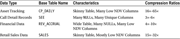
Hopefully, this data gives you some feel for the range of compression ratios that you can expect from HCC and the types of datasets that will benefit most. Of course, the best way to predict how compressible a particular table may be is to actually test it. This fact cannot be overemphasized.
There are a few challenges with using HCC. Many of them have to do with the fact that HCC is not available on most non-Exadata platforms. This fact makes for interesting scenarios for recovery and high-availability solutions. The other major challenge is that HCC does not play well with data that is being actively updated. In particular, systems characterized by lots of single-row updates, which we often describe as OLTP workloads, will probably not work well with HCC, even in 12c, which introduced row level locking.
Moving Data to a Non-Exadata Platform
Probably the largest hurdle with using HCC has been moving the data to non-Exadata platforms. For example, while RMAN and Data Guard both support the HCC block format and will happily restore data to a non-Exadata environment, a database running on such an environment will not be able to do anything with the data until it is decompressed. The only exception to this rule is the use of Oracle’s ZFS Storage Appliance, the FS1 storage system, or a Pillar Axiom array. Having to decompress data first can mean a lengthy delay before being able to access the data in a case where a failover to a standby on a non-Exadata platform occurs. The same issue holds true for doing an RMAN restore to a non-Exadata platform. The restore will work but the data in HCC formatted blocks will not be accessible until the data has been moved into a non-HCC format. This can be done with the ALTER TABLE MOVE NOCOMPRESS command, by the way.
![]() Note The ability to decompress HCC data on non-Exadata platforms only became available in Oracle database version 11.2.0.2. Attempting this on version 11.2.0.1 would result in an error.
Note The ability to decompress HCC data on non-Exadata platforms only became available in Oracle database version 11.2.0.2. Attempting this on version 11.2.0.1 would result in an error.
In addition to the lengthy delay associated with decompressing data before being able to access it, there is also the issue of space. If HCC is providing a 10× compression factor, for example, you will need to have 10 times the space you are currently using available on the target environment to handle the increased size of the data. For these reasons, Data Guard is rarely set up with a standby on a non-Exadata platform.
Before Oracle 12c, it was problematic to import HCC compressed data into a non-Exadata database. One long requested feature has been added to impdp, allowing the DBA to specify the compression level on the fly, as in this example:
[oracle@nonExadata ~]$ impdp user/password@nonExadata/testpdb1
> directory=data_pump_dir dumpfile=hcc_dump.dmp
> transform=table_compression_clause:nocompress
Before importing the previously HCC compressed table, you need to ensure that you have enough storage space for the import to succeed. Failing to provide the transformation clause when importing to a non-Exadata system will cause the import to abort with the following error message:
Processing object type TABLE_EXPORT/TABLE/TABLE
ORA-39083: Object type TABLE:"MARTIN"."UPDTEST_QL" failed to create with error:
ORA-64307:  Exadata Hybrid Columnar Compression is not supported for tablespaces on
  this storage type
Disabling Serial Direct Path Reads
As you saw in Chapter 2, serial Direct Path Reads allow non-parallelized scan operations to use the direct path read mechanism, which is a prerequisite for enabling the Smart Scan features of Exadata. Serial Direct Path Reads are enabled based on a calculation that depends on the size of the object being scanned relative to the available buffer cache. In simplistic terms, only large objects will be considered for Serial Direct Path Reads. HCC’s effectiveness can actually work against it here. Since the compression reduces the size of the objects so drastically, it can cause statements that would normally benefit from a Smart Scan to use the standard read mechanism, disabling many of Exadata’s optimizations. This is generally not a huge problem because the number of blocks is considerably reduced by HCC.
The database is making the decision to use a Direct Path Read (leading to a Smart Scan) at runtime. This can become interesting when an object is compressed and partitioned. The algorithm to use a Smart Scan or not is based on the size of the object being scanned; in the case of a partitioned object, this means the size of the partition. So in cases where partitioning is used with HCC, we often see some partitions using Smart Scans and some unable to use Smart Scans. Keep in mind that not using Smart Scans also means decompression cannot be done at the storage layer, as this capability is enabled only when performing Smart Scans.
Locking Issues
The documentation used to read that updating a single row of a table compressed with HCC locks the entire CU containing the row. This can cause extreme contention issues for OLTP-type systems. Not that you would want to compress active data with HCC anyway, for reasons already laid out earlier in this chapter.
Locking the entire CU for us is the main reason that HCC is not recommended for tables (or partitions) where the data will be updated. This has changed with Oracle 12c.. If you like, you can set some space in the CU header aside for tracking DML. To enable this feature, you have to specify the new syntax for HCC, as in this example:
CREATE TABLE t1_ql_rll
enable row movement
column store compress for query low row level locking
AS
select * from t1_ql;

Table created.
Table T1_QL_RLL has been created with one million random rows using Query Low as the compression mechanism. Row level locking really works best (if you can say so) with Query Compression. Its effects are somewhat unpredictable in Archive Compression mode. But then that makes perfect sense. Archived data should not be updated in the first place, should it? Comparing the two tables yields an interesting result:
SQL> select table_name,compression,compress_for,last_analyzed
  2  from tabs where table_name like 'T1_QL%';

TABLE_NAME           COMPRESS COMPRESS_FOR                   LAST_ANAL
-------------------- -------- ------------------------------ ---------
T1_QL                ENABLED  QUERY LOW                      22-AUG-14
T1_QL_RLL            ENABLED  QUERY LOW ROW LEVEL LOCKING    22-AUG-14
First of all, you can see that row level locking has been requested and applied to the table. When you compare the table sizes, then you will notice that the extra space in the CU header, which is required to keep track of the DML operations, takes a little toll:
SQL> select segment_name,bytes/power(1024,2) m, blocks
  2  from user_segments
  3  where segment_name like 'T1_QL%';

SEGMENT_NAME                  M     BLOCKS
-------------------- ---------- ----------
T1_QL                       176      22528
T1_QL_RLL                   192      24576
In this small example with a measly one million rows, the size difference is a few MB. The information about locked rows is not hidden in the first few bytes of the CU. As one might expect, it is clearly visible in the CU header. Dumping a block with a random CU header gives it away:
data_block_dump,data header at 0x7efefa13407c
===============
tsiz: 0x1f80
hsiz: 0x1c
pbl: 0x7efefa13407c
     76543210
flag=-0------
ntab=1
nrow=1
frre=-1
fsbo=0x1c
fseo=0x5e8
avsp=0x5cc
tosp=0x5cc
        r0_9ir2=0x0
        mec_kdbh9ir2=0x0
                      76543210
        shcf_kdbh9ir2=----------
                  76543210
        flag_9ir2=--R-----      Archive compression: Y
                fcls_9ir2[0]={ }
0x16:pti[0]     nrow=1  offs=0
0x1a:pri[0]     offs=0x5e8
block_row_dump:
tab 0, row 0, @0x5e8
tl: 6552 fb: --H-F--N lb: 0x0  cc: 1
nrid:  0x0140219c.0
col  0: [6540]
Compression level: 01 (Query Low)
 Length of CU row: 6540
kdzhrh: ------PCL CBLK: 2 Start Slot: 00
 NUMP: 02
 PNUM: 00 POFF: 5617 PRID: 0x0140219c.0
 PNUM: 01 POFF: 13633 PRID: 0x0140219d.0
num lock bits: 7
locked rows:
*---------
CU header:
CU version: 0   CU magic number: 0x4b445a30
CU checksum: 0x22424f63
CU total length: 17189
CU flags: NC-U-CRD-OP
ncols: 6
nrows: 1015
algo: 0
CU decomp length: 17016   len/value length: 1049278
row pieces per row: 1
num deleted rows: 0
START_CU:
 00 00 19 8c 4f 02 00 00 00 02 00 00 15 f1 01 40 21 9c 00 00 00 00 35 41 01
In this particular CU, you can see 7 lock bits for locking rows. The next line actually shows you the locked rows (if any). Now let’s try and update some rows in a compression unit and dump the block. But before that can be done, block numbers for the rows to be updated have to be found. Using the following query, they can be identified in block 192700 for IDs 1 to 78:
SQL> select min(id),max(id),blockn from (
  2    select id,DBMS_ROWID.ROWID_RELATIVE_FNO(rowid),
  3     DBMS_ROWID.ROWID_BLOCK_NUMBER(rowid) as blockn
  4     from martin.t1_ql_rll where id < 2500
  5  ) group by blockn order by blockn;

   MIN(ID)    MAX(ID)     BLOCKN
---------- ---------- ----------
         1         78     192700
        79        708       8603
       169        258       8689
       259        348      26064
       349        438     173609
       439        528     173715
       529        570     173860
       571        618     196434
       709       2499       8641
       841       1464       8646
      1465       2220      26012
In the next step, a transaction is started with an update against IDs 1 through 10:
SQL> update t1_ql_rll set spcol = 'me me me' where id between 1 and 10;

10 rows updated.
And now for the big moment—the block dump for this block shows this:
Block header dump:  0x01c04d40
 Object id on Block? Y
 seg/obj: 0x56ef  csc: 0x00.2385ed  itc: 3  flg: E  typ: 1 - DATA
     brn: 0  bdba: 0x1c04a03 ver: 0x01 opc: 0
     inc: 0  exflg: 0

 Itl           Xid                  Uba         Flag  Lck        Scn/Fsc
0x01   0xffff.000.00000000  0x00000000.0000.00  C---    0  scn 0x0000.002385ed
0x02   0x000a.00c.0000127a  0x000009f3.033b.0a  ----   10  fsc 0x0000.00000000
0x03   0x0000.000.00000000  0x00000000.0000.00  ----    0  fsc 0x0000.00000000
bdba: 0x01c04d40
data_block_dump,data header at 0x7f2fa276307c
[...]
tab 0, row 1, @0x2ea
tl: 3465 fb: --H-F--N lb: 0x0  cc: 1
nrid:  0x01c04d41.0
col  0: [3453]
Compression level: 01 (Query Low)
 Length of CU row: 3453
kdzhrh: ------PCL CBLK: 4 Start Slot: 00
 NUMP: 04
 PNUM: 00 POFF: 2020 PRID: 0x01c04d41.0
 PNUM: 01 POFF: 10036 PRID: 0x01c04d42.0
 PNUM: 02 POFF: 18052 PRID: 0x01c04d43.0
 PNUM: 03 POFF: 26068 PRID: 0x01c04d44.0
num lock bits: 6
locked rows: 1040(2), 1041(2), 1042(2), 1043(2), 1044(2), 1045(2), 1046(2), 1047(2), 1048(2), 1049(2),
*---------
CU header:
The header information reflects the updated blocks. What does this imply for concurrency? In the following example—without row level locking—the well-known behavior where the whole CU is locked can be observed:
Session1> update t1_ql set spcol = 'UPDATED' where id between 1 and 10;

10 rows updated.

Elapsed: 00:00:00.06

Session2> update t1_ql set spcol='UPDATED TOO' where id between 100 and 110;

-- session waits
As you would expect, session 2 has to wait until session 1 commits. No surprises, this is the expected behavior:
SQL> select sid,serial#,sql_id,seq#,event from v$session where username = 'MARTIN';

       SID    SERIAL# SQL_ID              SEQ# EVENT
---------- ---------- ------------- ---------- --------------------------------------------
       328       1679 fvcbzbm0gak1x         91 SQL*Net message to client
      1109      13459 39pvvwpfpfcum         52 enq: TX - row lock contention
If you repeat the test with the table that has row level locking enabled, you will see the two updates just pass as with a regular table:
Session1> update t1_ql_rll set spcol = 'UPDATED' where id between 1 and 10;

10 rows updated.

Elapsed: 00:00:00.04

Session2> update t1_ql_rll set spcol='UPDATED TOO' where id between 100 and 110;

11 rows updated.

Elapsed: 00:00:00.03
No waits, no locks in this case. Now before you start redefining all your tables, please consider the principles around HCC and active data. Just because there is support for row level locking, other DML operations are still better not issued against HCC compressed data.
Single Row Access
HCC is built and best suited for full-table scans. Decompression is a CPU-intensive task. Smart Scans can distribute the decompression work to the CPUs on the storage cells. This makes the CPU-intensive task much more palatable. However, Smart Scans only occur when Full Scans are performed. This means that other access mechanisms, index access for example, must use the DB server CPUs to perform decompression. In extreme cases, this can put an enormous CPU load on database servers, for example in high volume OLTP-type systems. In addition, since data for a single row is spread across multiple blocks in a CU, retrieving a complete row causes the entire CU to be read. This can have a detrimental effect on the overall database efficiency for systems that tend to access data using indexes, even if the access is read-only.
Common Usage Scenarios
HCC provides such high levels of compression that it has been used as an alternative to traditional Information Lifecycle Model (ILM) strategies, which generally involve moving older historical data off the database entirely. These ILM strategies usually entail some type of date range partitioning and a purge or archiving process. This is done to free storage and, in some cases, to improve performance. Often the data must be retained in some backup format so that it can be accessed if required at some later date. With HCC, it is possible in many cases to retain data almost indefinitely by compressing the oldest partitions. This approach has many advantages over the traditional approach of moving the data.
First and foremost, the data remains available via the standard application interfaces. No additional work will need to be done to restore a backup of old data before it can be accessed. This advantage alone is often enough to justify this approach. This approach typically entails leaving active partitions uncompressed while compressing old partitions more aggressively. Here’s a short example of creating a partitioned table with mixed compression modes using the 11.2 syntax:
SQL>   CREATE TABLE "KSO"."CLASS_SALES_P"
  2     (    "TRANS_ID" VARCHAR2(30),
  3          "UNIT_ID" NUMBER(30,0),
  4          "DAY" NUMBER(30,0),
  5          "TRANS_SEQ" VARCHAR2(30),
  6          "END_DATE" DATE,
  7          "BEGIN_DATE" DATE,
  8          "UNIT_TYPE" VARCHAR2(30),
  9          "CUST_TYPE" VARCHAR2(1),
 10          "LOAD_DATE" DATE,
 11          "CURRENCY_TYPE" CHAR(1)
 12     ) PCTFREE 10 PCTUSED 40 INITRANS 1 MAXTRANS 255  NOLOGGING
 13    STORAGE(
 14    BUFFER_POOL DEFAULT FLASH_CACHE DEFAULT CELL_FLASH_CACHE DEFAULT)
 15    TABLESPACE "CLASS_DATA"
 16    PARTITION BY RANGE ("BEGIN_DATE")
 17   (PARTITION "P1"  VALUES LESS THAN (TO_DATE
 18      (' 2008-09-06 00:00:00', 'SYYYY-MM-DD HH24:MI:SS', 'NLS_CALENDAR=GREGORIAN'))
 19  SEGMENT CREATION IMMEDIATE
 20    PCTFREE 10 PCTUSED 40 INITRANS 1 MAXTRANS 255 NOCOMPRESS NOLOGGING
 21    STORAGE(INITIAL 8388608 NEXT 1048576 MINEXTENTS 1 MAXEXTENTS 2147483645
 22    PCTINCREASE 0 FREELISTS 1 FREELIST GROUPS 1 BUFFER_POOL DEFAULT
 23    FLASH_CACHE DEFAULT CELL_FLASH_CACHE DEFAULT)
 24    TABLESPACE "CLASS_DATA" ,
 25   PARTITION "P2"  VALUES LESS THAN (TO_DATE
 26     (' 2008-09-07 00:00:00', 'SYYYY-MM-DD HH24:MI:SS', 'NLS_CALENDAR=GREGORIAN'))
 27  SEGMENT CREATION IMMEDIATE
 28    PCTFREE 0 PCTUSED 40 INITRANS 1 MAXTRANS 255 COMPRESS FOR QUERY HIGH NOLOGGING
 29    STORAGE(INITIAL 8388608 NEXT 1048576 MINEXTENTS 1 MAXEXTENTS 2147483645
 30    PCTINCREASE 0 FREELISTS 1 FREELIST GROUPS 1 BUFFER_POOL DEFAULT
 31    FLASH_CACHE DEFAULT CELL_FLASH_CACHE DEFAULT)
 32    TABLESPACE "CLASS_DATA" ,
 33   PARTITION "P3"  VALUES LESS THAN (TO_DATE
 34     (' 2008-09-08 00:00:00', 'SYYYY-MM-DD HH24:MI:SS', 'NLS_CALENDAR=GREGORIAN'))
 35  SEGMENT CREATION IMMEDIATE
 36    PCTFREE 0 PCTUSED 40 INITRANS 1 MAXTRANS 255 COMPRESS FOR ARCHIVE LOW NOLOGGING
 37    STORAGE(INITIAL 8388608 NEXT 1048576 MINEXTENTS 1 MAXEXTENTS 2147483645
 38    PCTINCREASE 0 FREELISTS 1 FREELIST GROUPS 1 BUFFER_POOL DEFAULT
 39    FLASH_CACHE DEFAULT CELL_FLASH_CACHE DEFAULT)
 40    TABLESPACE "CLASS_DATA" ) ;

Table created.
Oracle 12c introduces a new feature (as a cost option) to automate the data lifecycle management process, which is introduced in the next section.
Oracle Data Optimization (ADO) is a new feature introduced in version 12.1.0.1. It is available for Exadata, but is not limited to it. ADO helps the administrator implement, and more importantly, enforce Information Lifecycle Management if the Advanced Compression Option is available.
What Is Data Lifecycle Management?
Data lifecycle management is an important aspect of managing data and storage effectively. In many companies you will find different tiers of storage for non-Exadata deployments. Most commonly, you find Flash memory as tier 0 or 1, depending on where you start counting. The highest-level storage tier gives the user the best possible performance while, at the same time, is not available in abundance. Most tier 0 storage is too expensive to use throughout the board. And it is not even needed: a Data Warehouse deployed entirely on Flash memory makes little sense thanks to the data access patterns we observe.
Many warehouses are (incrementally) loaded during the day. Oracle architects and application designers alike have found partitioning the tables in an Oracle Data Warehouse by range, based on a date-key, very efficient. Numerous blog posts and presentations exist demonstrating how to scale effectively with that approach. Fellow Oak-Table member Tim Gorman’s paper “Scaling to Infinity: Data Warehouse on Oracle” gives a very good overview of how the partitioning option can be used to scale Oracle performance for Very Large Databases (VLDBs). So, where it is possible to partition the table into range-based segments, data lifecycle management is the natural next step to implement. It is nothing new. In fact, administrators have frequently implemented it to save costs a long time before Exadata saw the light of day.
While data is “hot,” or, in other words, freshly loaded, you can expect most activity. The load itself will require sufficient bandwidth to move the data from the staging layer into the query layer where it can be accessed by end users. You need to cater not only for the load but anything Oracle will perform in order to make the data available. Creating or maintaining indexes are the most visible operations during the load, but you can equally find redo and undo generation among the tasks Oracle performs, including writing to the archived logs if the database is in archivelog mode and enforces logging. Most systems are not quiesced during the load so you need to think about query performance as well; reading from storage you are processing your ETL is most likely to happen concurrently. In summary, I/O requirements are very demanding for current data.
Once the data becomes colder over time, access to it is not as thunderous and demanding. Most query activity focuses on current data. Many architects, therefore, decide to move data, which is not as frequently queried or modified to lower tiers of storage.
Continuing with the tier-0 example (Flash memory), many users move to hard-disk-based storage. These hard disks do not offer the same high-end performance characteristics as flash memory, but they are a lot cheaper in exchange.
Finally, over time, colder data can be moved to even lower tiers of storage. This allows the administrators and architects to retain larger amounts of data at lower cost than would have been possible by keeping everything on higher tier SAN storage.
Compression
So far, we have primarily focused on how to reduce cost with longer- or long-term archiving. The topic of compression has not been touched yet, but since this book is about Exadata, it inevitably has to be mentioned.
On the Exadata platform, you do not use these storage tiers as you would on traditional hardware. The Exadata administrator does not need to worry about the exact right combination of Flash Memory/SAN based tier 2 and 3 storage/network-based solutions. Storage is provided with the system. If you want to keep everything on the storage servers, while at the same time data volumes are growing, you should seriously consider HCC. You read in the previous sections that HCC can give you very good compression ratios and, therefore, savings in your storage footprint. In addition to these, you can use Smart-Scans on HCC compressed data, enhancing throughput significantly compared to non-Exadata platforms. Accessing HCC compressed data via Infiniband should be more efficient than accessing data based on a Direct NFS (dNFS) filer, for example.
Automatic Data Optimization vs. Manual Lifecycle Management
Before Oracle 12c, it was the DBA’s task to perform housekeeping. In many cases, housekeeping included implementing an ILM policy. With properly implemented change management, this used to work well. In situations where change management was not as rigorously implemented, however, it could become difficult to maintain the ILM policy.
Oracle 12c relieves the DBA from many of these tasks by allowing the application of the ILM policy to happen automatically. As you can see in the next sections, you can add a declarative policy to a segment and leave the implementation to Oracle. This feature requires the Advanced Compression License.
ADO is largely based on usage tracking. A so-called heat map tracks access and data modification at the row and segment level. Not only is the heat map the basis for ADO, it can also be queried using data dictionary views and manipulated via a set of PL/SQL Application Programming Interfaces (APIs).
The administrator—broadly speaking—is given two options that thankfully are not mutually exclusive. The first option is to compress; the other option is to use the tiering clause. The first step, though, is to enable the heat map. However, be careful: Enabling the heat map tracking already requires you to have a license for the Advanced Compression Option.
SQL> alter system set heat_map = on sid='*' scope=both;

System altered.
Oracle offers a number of views you can use to find out more about the heat map tracking in your database:
SQL> SELECT table_name
  2  FROM dict
  3  WHERE table_name LIKE 'V%HEAT%MAP%'
  4  OR table_name LIKE 'DBA%HEAT%MAP%';

TABLE_NAME
------------------------------
DBA_HEATMAP_TOP_OBJECTS
DBA_HEATMAP_TOP_TABLESPACES
DBA_HEAT_MAP_SEG_HISTOGRAM
DBA_HEAT_MAP_SEGMENT
V$HEAT_MAP_SEGMENT
V$HEAT_MAP_SEGMENT is the dictionary view that provides real-time access to the heat map, but does not feature a “owner” column such as DBA_HEATMAP_TOP_OBJECTS. You can easily join against DBA_OBJECTS on the OBJECT_ID and DATA_OBJECT_ID.
Example Use Cases for ADO
To better illustrate the concepts and implementation of ADO, the following demonstration will be used. A simple table named ADODEMO will serve for this purpose. A number of Information Lifecycle Management policies will be attached to it and their effect shown. Let’s begin with the table definition:
CREATE TABLE adodemo (
 id, t_pad, date_created, state
)
enable row movement
partition by range (date_created)
INTERVAL(NUMTOYMINTERVAL(1, 'MONTH'))
(
 partition p_manual values less than (to_date('01.01.2005','dd.mm.yyyy'))
)
AS -- thank you Jonathan Lewis!
WITH v1 AS  (
  SELECT rownum n FROM dual CONNECT BY level <= 10000
)
SELECT
  rownum id,
  rpad(rownum,1999) t_pad,
  TRUNC(sysdate) - 180 + dbms_random.value(0,180) date_created,
  CASE
    WHEN mod(rownum,100000) = 0
    THEN CAST('RARE' AS VARCHAR2(12))
    WHEN mod(rownum,10000) = 0
    THEN CAST('FAIRLY RARE' AS VARCHAR2(12))
    WHEN mod(rownum,1000) = 0
    THEN CAST('NOT RARE' AS VARCHAR2(12))
    WHEN mod(rownum,100) = 0
    THEN CAST('COMMON' AS   VARCHAR2(12))
    ELSE CAST('THE REST' AS VARCHAR2(12))
  END state
FROM v1,
  v1
WHERE rownum <= 1e7;
The table has ten million rows but is rather narrow. The ADODEMO table is primarily interesting from a partitioning aspect. You read in the previous section how important partitioning was for a suitable implementation of HCC. Notice that the table does not have compression enabled at all initially. This is intentional: With ADO, you do not need to specify the compression yourself—leave that to Oracle. In our 12.1.0.2.0 test bed, the table had these physical properties:
SQL> select table_name,partition_name,num_rows,last_analyzed
  2  from dba_tab_partitions where table_owner = 'MARTIN' and table_name = 'ADODEMO';

TABLE_NAME                     PARTITION_NAME         NUM_ROWS LAST_ANAL
------------------------------ -------------------- ---------- ---------
ADODEMO                        P_MANUAL
ADODEMO                        SYS_P796                1721062 09-OCT-14
ADODEMO                        SYS_P797                1111364 09-OCT-14
ADODEMO                        SYS_P798                1724376 09-OCT-14
ADODEMO                        SYS_P799                1664931 09-OCT-14
ADODEMO                        SYS_P800                1720722 09-OCT-14
ADODEMO                        SYS_P801                 389333 09-OCT-14
ADODEMO                        SYS_P802                1668212 09-OCT-14

8 rows selected.
Thanks to the interval partitioning on MONTH, you do not need to concern yourself with the partitioning definition in too much detail. A single default partition is enough; Oracle will create new partitions when needed.
Enable ILM for Storage Tiering
You already read that Oracle allows you to automate the movement of “cold” data from tier-1 storage to lower tiers automatically based on so-called ILM policies. These policies can be assigned to a table at creation time or alternatively retrofitted. It is possible to define the policies on the row or segment.
First of all, a target to move the data to is required. In the example, it is a tablespace named ILM_COMPRESS. The source tablespace name is MARTIN_BIGFILE. Currently, every segment of table ADODEMO is found on that tablespace as a query against DBA_TAB_PARTITIONS reveals:
TABLESPACE_NAME                PARTITION_NAME
------------------------------ --------------
MARTIN_BIGFILE                 P_MANUAL
MARTIN_BIGFILE                 SYS_P796
MARTIN_BIGFILE                 SYS_P797
MARTIN_BIGFILE                 SYS_P798
MARTIN_BIGFILE                 SYS_P799
MARTIN_BIGFILE                 SYS_P800
MARTIN_BIGFILE                 SYS_P801
MARTIN_BIGFILE                 SYS_P802
Now you can add the ILM policy to the oldest partition.
SQL> alter table ADODEMO modify partition SYS_P797
  2  ilm add policy tier to ILM_COMPRESS;

Table altered.

SQL> select policy_name,object_name,subobject_name,enabled from user_ilmobjects;

POLICY_NAME                    OBJECT_NAME                    SUBOBJECT_NAME                 ENA
------------------------------ ------------------------------ ------------------------------ ---
P1                             ADODEMO                        SYS_P797                       YES

1 row selected.
You just saw one of the dictionary views related to Information Lifecycle Management in action: USER_ILMOBJECTS. This view lists all the objects to which an ILM policy has been attached. Before anything can happen to the example table, certain conditions need to be met. You can find the ILM parameters as currently defined in the view DBA_ILMPARAMETERS:
SQL> select * from DBA_ILMPARAMETERS;

NAME                      VALUE
-------------------- ----------
ENABLED                       1
RETENTION TIME               30
JOB LIMIT                     2
EXECUTION MODE                2
EXECUTION INTERVAL           15
TBS PERCENT USED             85
TBS PERCENT FREE             25
POLICY TIME                   0

8 rows selected.
With regards to storage tiering, only one parameter is of interest initially. TBS PERCENT USED is the threshold indicating when a “data move” policy should be implemented. Translated into English it means that a data move may occur when the tablespace on which the segment resides reaches more than 85% usage. Continuing the above example, the tablespace is over that threshold, which should trigger the data move.
Tablespace                      Size (MB)  Free (MB)     % Free     % Used
------------------------------ ---------- ---------- ---------- ----------
MARTIN_BIGFILE                     209920  6403.4375          3         97
The evaluation of ILM policies is performed as part of the maintenance job window overnight. For most systems, that should be 10 p.m., unless the scheduler windows have been changed. If you are in a hurry, you can speed the process on your development environment up by invoking the EXECUTE_ILM procedure in the DBMS_ILM package. One of its parameters is an out variable named task_id. It returns the automatically created name of the task associated with the execution of ILM policies.
You can use the command print task_id in your SQL*Plus session to get the actual value of the task. By invoking DBMS_ILM.EXECUTE_ILM, you execute ILM policies in the current schema. The outcome of the policy evaluation is in another new dictionary view, named USER_ILMEVALUATIONDETAILS:
SQL> select selected_for_execution, job_name, policy_name
  2  from user_ilmevaluationdetails
  3   where task_id = :task_id
  4  /

SELECTED_FOR_EXECUTION         JOB_NAME                       POLICY_NAME
------------------------------ ------------------------------ ---------------
SELECTED FOR EXECUTION         ILMJOB408                      P1
In this case, the policy has been selected for execution. To know more about the outcome of the data move, you can check USER_ILMRESULTS:
SQL> select job_state,start_time,completion_time from USER_ILMRESULTS
  2  where task_id = :task_id and job_name = 'ILMJOB408';

JOB_STATE                START_TIME                     COMPLETION_TIME
------------------------ ------------------------------ ------------------------------
COMPLETED SUCCESSFULLY   08-OCT-14 10.00.42.603455 PM   08-OCT-14 10.00.55.250004 PM
The job’s execution is also recorded in the scheduler views, such as DBA_SCHEDULER_JOB_RUN_DETAILS. Under the covers, Oracle executes a PL/SQL block, which is recorded in SYS.ILM_RESULTS$ if you are interested at having a look. The actual code executed by the database is stored in the PAYLOAD column. The dictionary view already suggested that the job’s execution succeeded, but you can see the effect yourself. Going back to USER_TAB_PARTITIONS, you see that the tablespace name for the partition changed:
SQL> select partition_name,tablespace:name from user_tab_partitions
  2  where table_name = 'ADODEMO' and partition_name = 'SYS_P797';

PARTITION_NAME                 TABLESPACE_NAME
------------------------------ ---------------
SYS_P797                       ILM_COMPRESS

1 row selected.
As another expected side effect, you get some more free space in the original tablespace as well. The storage tiering option is quite useful in Exadata, especially if you are using the ZFS Storage Appliance or a Pillar Axiom/FS1 array as a target for the data move. Keep in mind that neither of these allows you to Smart Scan the data on it. On the other hand, data that is moved to such a tablespace may be cold and not accessed frequently anyway.
Another option that has already been alluded to allows you to compress data as it gets cold. The heat map is instrumental to this functionality. Without it, Oracle could not possibly keep track of data access and manipulation. And because Oracle kernel developers have a heart for DBAs, they even added some statistics to signal its usage to the performance architect:
SQL> select name from v$statname where lower(name) like '%heat%';

NAME
----------------------------------------------------------------
Heatmap SegLevel - Write
Heatmap SegLevel - Full Table Scan
Heatmap SegLevel - IndexLookup
Heatmap SegLevel - TableLookup
Heatmap SegLevel - Flush
Heatmap SegLevel - Segments flushed
Heatmap BlkLevel Tracked
Heatmap BlkLevel Not Tracked - Memory
Heatmap BlkLevel Not Updated - Repeat
Heatmap BlkLevel Flushed
Heatmap BlkLevel Flushed to SYSAUX
Heatmap BlkLevel Flushed to BF
Heatmap BlkLevel Ranges Flushed
Heatmap BlkLevel Ranges Skipped
Heatmap BlkLevel Flush Task Create
Heatmap Blklevel Flush Task Count

16 rows selected.
When you use co-author Tanel Poder’s snapper to capture the change performance counters over time, you might actually start seeing some of these! To simulate access to the data-table ADODEMO, a small procedure has been written:
create or replace procedure ADODEMOPROC as
  v_id number;
  v_date date;
begin
  v_date :=  to_date('01-AUG-2014') + dbms_random.value(1,10);
  select count(id) into v_id from martin.adodemo where date_created = trunc(v_date);
end;
/
The intention is to use that query in a number of scheduler jobs to simulate user activity. This activity is needed for the next example to work as expected. Since the above query performed a full scan initially, an index was added on the DATE_CREATED column. The scheduler jobs are created by calling DBMS_SCHEDULER directly:
SQL> begin
  2    for i in 1..5 loop
  3      dbms_scheduler.create_job(
  4        job_name => 'ADODEMOJOB_' || i,
  5        job_type => 'STORED_PROCEDURE',
  6        job_action => 'ADODEMOPROC',
  7        start_date => systimestamp,
  8        repeat_interval => 'freq=secondly;interval=10',
  9        enabled => true);
 10    end loop;
 11  end;
 12  /

PL/SQL procedure successfully completed.
The ILM policy is the missing piece in the demonstration. As you can see in this example, the policy can be assigned to the table as a whole, and it will be inherited by the subpartitions:
SQL> alter table adodemo
  2  ilm add policy column store compress for query low
  3  segment after 30 days of no access;

Table altered.

SQL> select policy_name, subobject_name, object_type, inherited_from, enabled
  2  from user_ilmobjects where object_name = 'ADODEMO';

POLICY_NAM SUBOBJECT_NAME                 OBJECT_TYPE        INHERITED_FROM       ENA
---------- ------------------------------ ------------------ -------------------- ---
P1         SYS_P797                       TABLE PARTITION    POLICY NOT INHERITED NO
P3         P_MANUAL                       TABLE PARTITION    TABLE                YES
P3         SYS_P796                       TABLE PARTITION    TABLE                NO
P3         SYS_P797                       TABLE PARTITION    TABLE                YES
P3         SYS_P798                       TABLE PARTITION    TABLE                YES
P3         SYS_P799                       TABLE PARTITION    TABLE                YES
P3         SYS_P800                       TABLE PARTITION    TABLE                YES
P3         SYS_P801                       TABLE PARTITION    TABLE                YES
P3         SYS_P802                       TABLE PARTITION    TABLE                YES
P3                                        TABLE              POLICY NOT INHERITED YES

10 rows selected.
Policy P1 is the data-move policy implemented and executed in the previous section. Policy names are not user-definable. In other words, Oracle assigns them. Policy P3 is the new policy just added with the above command. As described in the previous paragraph, you can see the partitions have inherited the policy that has been assigned to the table. The scope of the policy is the data segment, or the partition in the case of a heap table. Just as with the storage tiering policy the new policy is evaluated with the opening of the maintenance window.
The outcome of the evaluation is again recorded in USER_ILMEVALUATIONDETAILS. It is possible that your segment is selected for execution, as shown here:
SQL> select policy_name POLICY, object_name "TABLE", subobject_name "PARTITION",
  2   selected_for_execution, job_name
  3  from user_ilmevaluationdetails;

POLICY     TABLE      PARTITION       SELECTED_FOR_EXECUTION                     JOB_NAME
---------- ---------- --------------- ------------------------------------------ ----------
P3         ADODEMO    SYS_P796        SELECTED FOR EXECUTION                     ILMJOB428
P1         ADODEMO    SYS_P797        PRECONDITION NOT SATISFIED
P3         ADODEMO    SYS_P797        PRECONDITION NOT SATISFIED
P3         ADODEMO    SYS_P798        PRECONDITION NOT SATISFIED
...
You can verify the job’s completion in USER_ILMRESULTS. The payload in SYS.ILM_RESULTS$ reveals another PL/SQL block compressing the partition. Once the job has completed successfully, you should be able to see the result in the dictionary:
SQL> select partition_name, table_name, compression, compress_for
  2    from user_tab_partitions
  3   where table_name = 'ADODEMO'
  4    and partition_name = 'SYS_P796';

PARTITION_NAME       TABLE_NAME                     COMPRESS COMPRESS_FOR
-------------------- ------------------------------ -------- ------------------------------
SYS_P796             ADODEMO                        ENABLED  QUERY LOW
This is a short introduction to what you can do with the ADO option. There are many more options available such as using custom functions for tiering. Like so many great Oracle features, the use of Automatic Data Optimization requires you to have an additional cost license (Advanced Compression).
Summary
Introduced in Oracle 11g Release 2, HCC provides exceptional compression capabilities that are far beyond anything available in prior releases. This is thanks in large part to the adoption of industry-standard compression algorithms and an increase in the size of the compression unit from a single database block (typically 8K) to a larger unit of 32K or 64K. Despite the enhancements with row level locking in 12c, the feature is only appropriate for data that is no longer being modified, because of locking issues and the fact that updated rows are moved into a much less compressed format (OLTP compression format). For this reason, HCC should only be used with data that is no longer being modified (or only occasionally modified). Since compression can be defined at the partition level, it is common to see tables that have a mixture of compressed and uncompressed partitions. This technique can, in many cases, replace ILM approaches that require moving data to alternate storage media and then purging it from the database. With Oracle 12c, the data lifecycle management process can be automated.