![]()
Compute Node Layout
The term node is a fairly generic one that has many different meanings in the IT industry. For example, network engineers call any addressable device attached to their network a node. Unix administrators commonly use the term interchangeably with host or server. Oracle DBAs often refer to a database server that is a member of an RAC cluster as a node. Oracle’s documentation uses the term compute node when referring to the database server tier of the platform. In this chapter, we will discuss the various ways in which you can configure your Exadata compute nodes, whether they are members of an RAC cluster (nodes) or nonclustered (database servers).
It’s a common misconception that an Exadata rack must be configured as a single Oracle RAC cluster. This couldn’t be further from the truth. In its simplest form, the Exadata database tier can be described as a collection of independent database servers hardwired into the same storage and the same management networks. Each of these servers can be configured to run stand-alone databases completely independent of the others. However, this is not commonly done for two reasons—scalability and high availability. Oracle RAC has historically been used to provide node redundancy in the event of node or instance failure, but Oracle marketing has made it clear all along that the ability to scale-out has been an equally important goal. Traditionally, if we needed to increase database performance and capacity, we did so by upgrading server hardware. This method became so commonplace that the industry coined the phrase hardware refresh to describe it. This term can mean anything from adding CPUs, memory, or I/O bandwidth to a complete replacement of the server itself. Increasing performance and capacity in this way is referred to as scale-up. With Exadata’s ability to provide extreme I/O performance to the database server, bus speed is now the limiting factor for scale-up. So, what happens when you reach the limits of single-server capacity? The obvious answer is to add more servers. To continue to scale your application, you must scale-out, using Oracle RAC. Nonetheless, understanding that the database servers are not tied together in some proprietary fashion clarifies the highly configurable nature of Exadata.
In Chapter 14, we discussed various strategies for configuring Exadata’s storage subsystems to service specific database servers. In this chapter, we will take a look at ways the database tier may be configured to create clustered and nonclustered database environments that are well suited to meet the needs of your business.
Provisioning Considerations
Exadata is an extremely configurable platform. Determining the best configuration for your business will involve reviewing the performance and uptime demands of your applications as well as ensuring adequate separation for development, test, and production systems. Here are a few of the key considerations for determining the most suitable compute node layout to support your database environments:
- CPU Resources: When determining the optimal node layout for your databases, keep in mind that Exadata handles the I/O workload very differently from traditional database platforms. On non-Exadata platforms, the database server is responsible for retrieving all data blocks from storage to satisfy I/O requests from the applications. Exadata offloads a lot of this work to the storage cells. This can significantly reduce the CPU requirements of your database servers. Figuring out how much less CPU your databases will require is a difficult task because it depends, in part, on how much your database is utilizing parallel query and HCC compression, as well as how suitable your application SQL is to offloading. Some of the Smart Scan optimizations, such as decryption, predicate filtering, and HCC decompression, will reduce CPU requirements regardless of the type of application. (We covered these topics in detail in Chapters 2–6.)
- Systems requiring thousands of dedicated server connections can overwhelm the resources of a single machine. Spreading these connections across multiple compute nodes reduces the burden on the system’s process scheduler and allows the CPU to spend its time more effectively servicing client requests. Load-balancing connections across multiple compute nodes also improves the database’s capacity for handling concurrent connection requests.
- Memory Resources: Systems that require thousands of dedicated server connections can also put a burden on memory resources. Each dedicated server connection requires a slice of memory, whether or not the connection is actively being used. Spreading these connections across multiple RAC nodes allows the database to handle more concurrent connections than a single compute node can manage.
- I/O Performance and Capacity: Each compute node and storage cell is equipped with one 40Gbps QDR, dual-port InfiniBand card through which, in practicality, each compute node can transmit/receive a maximum of 3.2 gigabytes per second (6.4 gigabytes per second for X4-2 and X5-2 compute nodes). If this is sufficient bandwidth, the decision of moving to a multi-node RAC configuration may be more of an HA consideration. If you have I/O-hungry applications that require more throughput than one compute node can provide, RAC may be used to provide high availability as well as additional I/O capacity.
- Patching and Testing: Another key consideration in designing a stable database environment is providing a separate area where patches and new features can be tested before rolling them into production. For non-Exadata platforms, patching and upgrading generally involves O/S patches and Oracle RDBMS patches. Exadata is a highly complex database platform, consisting of several additional hardware and software layers that must be patched periodically, such as Cell Servers, ILOM firmware, InfiniBand switch firmware, InfiniBand network card firmware, and OFED drivers. As such, it is absolutely crucial that a test environment be isolated from critical systems to be used for testing patches.
Non-RAC Configuration
Compute nodes may be configured in a number of ways. If your application does not need the high availability or scale-out features of Oracle RAC, then Exadata provides an excellent platform for delivering high performance for stand-alone database servers. You can manage I/O service levels between independent databases (be it single instance or Oracle RAC) by configuring IORM (See Chapter 7 for more information about IORM). In a non-RAC configuration, the Oracle Grid Infrastructure is still configured for a cluster, but the Oracle database homes are linked for single-instance databases only. Because the Exadata storage servers provide shared storage for all of the compute nodes, a clustered set of ASM disk groups can be used to provide storage to all of the compute nodes. This configuration gives database administrators the flexibility of a cluster while still maintaining licensing requirements for single-instance databases.
It may seem counterintuitive to use a cluster for single-instance databases, but users running this configuration gain many benefits of running across shared storage while cutting down on the drawbacks of segmenting resources to an extreme. Even though your database servers may run stand-alone databases, they can still share Exadata storage (cell disks). This allows each database to make use of the full I/O bandwidth of the Exadata storage subsystem. Database placement is determined by strain placed on the compute node, not the ASM disk group that belongs to that compute node. Because ASM disk groups are shared, databases can be moved within the cluster with minimal effort. Also, migration to a full-fledged RAC configuration is very simple from this configuration—just relink the database homes and convert the database to support RAC.
For example, let’s say you have three databases on your server called SALES, HR, and PAYROLL. All three databases can share the same disk groups for storage. To do this, all three databases would have instance parameters as follows:
db_create_file_dest='+DATA'
db_recovery_file_dest='+RECO'
local_listener='<connect string of local host listener>'
remote_listener='<SCAN_HOSTNAME:1521>'
In Figure 15-1, we see all eight compute nodes in an Exadata full rack configuration running stand-alone databases. You will notice that storage is allocated exactly the same as in a clustered configuration. All nodes use the +DATA and +RECO disk groups, which are serviced by the clustered ASM instances. Each ASM instance shares the same set of ASM disk groups, which consist of grid disks from all storage cells. Because the ASM disk groups are shared across all of the compute nodes, the loss of a single node does not mean that the databases it serves must stay down. If adequate resources are available on the surviving compute nodes, single-instance databases can easily be migrated to those nodes to restore service. Clients connecting over the SCAN interface need no reconfiguration to connect.

Figure 15-1. Example of a non-RAC Exadata configuration
If separate disk groups were created for each compute node, administrators would have to choose database placement based on both compute node resources and the disk space available to that cluster. Because reconfiguration of storage on Exadata is not a quick process, splitting disk groups between nodes forces much more early planning. Also, individual storage servers would be forced to manage Flash Cache and resource management plans across multiple clusters, leading to extra overhead needed to manage resources. Finally, the number of grid disks created in a configuration utilizing separate disk groups makes the cluster much more difficult to manage—a full rack utilizing separate +DATA and +RECO ASM disk groups would require 2,688 grid disks. The configuration described above creates no additional grid disks apart from the standard 476.
Now that we’ve discussed how to run Exadata in a non-RAC configuration, let’s take a look at how a single rack can be carved into multiple clusters. But before we do that, we’ll take a brief detour and establish what high availability and scalability are.
High availability (HA) is a fairly well-understood concept, but it often gets confused with fault tolerance. In a truly fault-tolerant system, every component is redundant. If one component fails, another component takes over without any interruption to service. High availability also involves component redundancy, but failures may cause a brief interruption to service while the system reconfigures to use the redundant component. Work in progress during the interruption must be resubmitted or continued on the redundant component. The time it takes to detect a failure, reconfigure, and resume work varies greatly in HA systems. For example, active/passive Unix clusters have been used extensively to provide graceful failover in the event of a server crash. Now, you might chuckle to yourself when you see the words graceful failover and crash used in the same sentence (unless you work in the airline industry), so let me explain. Graceful failover, in the context of active/passive clusters, means that when a system failure occurs or a critical component fails, the resources that make up the application, database, and infrastructure are shut down on the primary system and brought back online on the redundant system automatically with as little downtime as possible. The alternative, and somewhat less graceful, type of failover would involve a phone call to your support staff at 3:30 in the morning. In active/passive clusters, the database and possibly other applications only run on one node at a time. Failover using this configuration can take several minutes to complete, depending on what resources and applications must be migrated. Oracle RAC uses an active/active cluster architecture. Failover on an RAC system commonly takes less than a minute to complete. True fault tolerance is generally very difficult and much more expensive to implement than high availability. The type of system and impact (or cost) of a failure usually dictates which is more appropriate. Critical systems on an airplane, space station, or a life-support system easily justify a fault-tolerant architecture. By contrast, a web application servicing the company’s retail storefront usually cannot justify the cost and complexity of a fully fault-tolerant architecture. Exadata is a high-availability architecture providing fully redundant hardware components. When Oracle RAC is used, this redundancy and fast failover is extended to the database tier.
When CPU, memory, or I/O resource limits for a single server are reached, additional servers must be added to increase capacity. The term scalability is often used synonymously with performance. That is, increasing capacity equals increasing performance. But the correlation between capacity and performance is not a direct one. Take, for example, a single-threaded, CPU-intensive program that takes 15 minutes to complete on a two-CPU server. Assuming the server isn’t CPU-bound, installing two more CPUs is not going to make the process run any faster. If it can only run on one CPU at a time, it will only execute as fast as one CPU can process it. Performance will only improve if adding more CPUs allows a process to have more uninterrupted time on the processor. Neither will it run any faster if we run it on a four-node cluster. However, scaling out to four servers could mean that we can run four copies of our program concurrently and get roughly four times the amount of work done in the same 15 minutes. To sum it up, scaling out adds capacity to your system. Whether or not it improves performance depends on how scalable your application is and how heavily loaded your current system is. Keep in mind that Oracle RAC scales extremely well for well-written applications. Conversely, poorly written applications tend to scale poorly.
Exadata can be configured as multiple RAC clusters to provide isolation between environments. This allows the clusters to be managed, patched, and administered independently. At the database tier, this is done in the same way you would cluster any ordinary set of servers using Oracle Clusterware. To configure storage cells to service-specific compute nodes, the cellip.ora file on each compute node lists the storage cells it will use. For example, the following cellip.ora file lists seven of the fourteen storage cells by their network address (remember that beginning with X4-2, compute nodes support active/active InfiniBand connections):
[db01:oracle:EXDB1] /home/oracle
> cat /etc/oracle/cell/network-config/cellip.ora
cell="192.168.10.17;192.168.10.18"
cell="192.168.10.19;192.168.10.20"
cell="192.168.10.21;192.168.10.22"
cell="192.168.10.23;192.168.10.24"
cell="192.168.10.25;192.168.10.26"
cell="192.168.10.27;192.168.10.28"
cell="192.168.10.29;192.168.10.30"
When ASM starts up, it searches the storage cells on each of these IP addresses for grid disks it can use for configuring ASM disk groups. Alternatively, cell security can be used to lock down access so that only certain storage cells are available for compute nodes to use. The cellip.ora file and cell security are covered in detail in Chapter 14.
To illustrate what a multi-RAC Exadata configuration might look like, let’s consider an Exadata X5-2 full rack configuration partitioned into three Oracle RAC clusters. A full rack gives us eight compute nodes and fourteen storage cells to work with. Consider an Exadata full rack configured as follows:
- One Production RAC cluster with four compute nodes and seven storage cells
- One Test RAC cluster with two compute nodes and three storage cells
- One Development RAC cluster with two compute nodes and four storage cells
Table 15-1 shows the resource allocation of these RAC clusters, each with its own storage grid. As you read this table, keep in mind that hardware is a moving target. These figures are from an Exadata X5-2. In this example, we used the high-capacity, 4TB disk drives.
Table 15-1. Cluster Resources

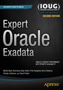
These RAC environments can be patched and upgraded completely independently of one another. The only hardware resource they share is the InfiniBand fabric. If you are considering a multi-RAC configuration like this, keep in mind that patches to the InfiniBand switches will affect all storage cells and compute nodes. Figure 15-2 illustrates what this cluster configuration would look like.
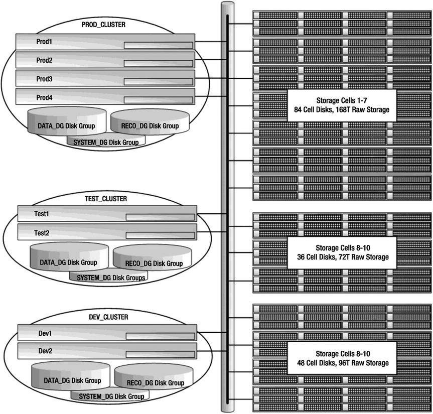
Figure 15-2. An Exadata full rack configured for three RAC clusters
The two configuration strategies we’ve discussed so far are fairly extreme examples. The non-RAC database configuration illustrated how Exadata can be configured without Real Application Clusters, creating a true consolidation platform. The second example, Split-RAC Clusters, showed how Clusterware can be used to create multiple, isolated RAC clusters. Neither of these configurations is typically found in the real world, but they illustrate the configuration capabilities of Exadata. Now let’s take a look at a configuration we commonly see in the field. Figure 15-3 shows a typical system with two Exadata half racks. It consists of a production cluster (PROD_CLUSTER) hosting a two-node production database and a two-node UAT database. The production and UAT databases share the same ASM disk groups (made up of all grid disks across all storage cells). I/O resources are regulated and prioritized using Exadata I/O Resource Manager (IORM), discussed in Chapter 7. The production database uses Active Data Guard to maintain a physical standby for disaster recovery and reporting purposes. The UAT database is not considered business-critical, so it is not protected with Data Guard. On the standby cluster (STBY_CLUSTER), the STBY database uses four of the seven storage cells for its ASM storage. On the development cluster (DEV_CLUSTER), the Dev database uses the remaining three cells for its ASM storage. The development cluster is used for ongoing product development and provides a test bed for installing Exadata patches, database upgrades, and new features.
Figure 15-3. A typical configuration
Exadata’s ability to scale out doesn’t end when the rack is full. When one Exadata rack doesn’t quite get the job done for you, additional racks may be added to the cluster, creating a large-scale database grid. Up to 18 racks may be cabled together to create a massive database grid, consisting of 144 database servers and over 12 petabytes of raw disk storage. Actually, Exadata will scale beyond 18 racks, but additional InfiniBand switches must be purchased to do it. Exadata utilizes a spine switch to link cabinets together (compute and storage servers connect directly to the leaf switches). The spine switch was included with all half rack and full rack X2-2 and X3-2 configurations. Beginning with the X4-2 model, the spine switch is an additional purchase. Unless a spine switch is purchased, quarter rack configurations can only be linked with one other Exadata rack. In a full rack configuration, the ports of a leaf switch are used as follows:
- Eight links to the database servers
- Fourteen links to the storage cells
- Seven links to the redundant leaf switch
- Seven ports open
Figure 15-4 shows an Exadata full rack configuration that is not linked to any other Exadata rack. It’s interesting that Oracle chose to connect the two leaf switches together using the seven spare cables. Perhaps it’s because these cables are preconfigured in the factory—patching them into the leaf switches simply keeps them out of the way and makes it easier to reconfigure later. The leaf switches certainly do not need to be linked together.

Figure 15-4. An Exadata full rack InfiniBand network
The spine switch is just like the other two InfiniBand switches that service the cluster and storage network, with one exception. The spine switch serves as the subnet manager master for the InfiniBand fabric. Redundancy is provided by connecting each leaf switch to every spine switch in the configuration (from two to eighteen spine switches).
To cable two Exadata racks together, the seven inter-switch cables, seen in Figure 15-4, are redistributed so that four of them link the leaf switch with its internal spine switch, and four of them link the leaf switch to the spine switch in the adjacent rack. Figure 15-5 shows the network configuration for two Exadata racks networked together. When eight Exadata racks are linked together, the seven inter-switch cables seen in Figure 15-4 are redistributed so that each leaf-to-spine-switch link uses one cable (eight cables per leaf switch). When you’re linking from three to seven Exadata racks together, the seven inter-switch cables are redistributed as evenly as possible across all leaf-to-spine-switch links. Leaf switches are not linked to other leaf switches, and spine switches are not linked to other spine switches. No changes are ever needed for the leaf switch links to the compute nodes and storage cells. This network topology is typically referred to as fat tree topology.

Figure 15-5. A switch configuration for two Exadata racks, with one database grid
Summary
Exadata is a highly complex, highly configurable database platform. In Chapter 14, we talked about all the various ways disk drives and storage cells can be provisioned separately or in concert to deliver well-balanced, high-performance I/O to your Oracle databases. In this chapter, we turned our attention to provisioning capabilities and strategies at the database tier. Exadata is rarely used to host stand-alone database servers. In most cases, it is far better suited for Oracle RAC clusters. Understanding that every compute node and storage cell is a fully independent component is important, so we spent a considerable amount of time showing how to provision eight stand-alone compute nodes on an Exadata full rack configuration. From there, we moved on to an Oracle RAC provisioning strategy that provided separation between three computing environments. And, finally, we touched on how Exadata racks may be networked together to build massive database grids. Understanding the concepts explored in Chapters 14 and 15 of this book will help you make the right choices when the time comes to architect a provisioning strategy for your Exadata database environment.