Offloading is the key differentiator of the Exadata platform and has sparked excitement with us since we laid hands on our first Exadata system. Offloading is what makes Exadata different from every other platform that Oracle runs on. The term offloading refers to the concept of moving processing from the database layer to the storage layer. It is also the key paradigm shift provided by the Exadata platform. But it is more than just moving work in terms of CPU usage. The primary benefit of offloading is the reduction in the volume of data that must be returned to the database server—one of the major bottlenecks of most large databases.

The terms offloading and Smart Scan are used somewhat interchangeably. Offloading is a better description in our opinion, as it refers to the fact that part of the traditional SQL processing done by the database can be “offloaded” from the database layer to the storage layer. It is a rather generic term, though, and is used to refer to many optimizations that are not even related to SQL processing, including improving backup and restore operations, file initialization, and more.

Smart Scan

, on the other hand, is a more focused term in that it refers only to Exadata’s optimization of SQL statements. These optimizations come into play for scan operations—typically full segment scans. A more specific definition of a Smart Scan would be any section of the Oracle kernel code that is covered by the Smart Scan wait events. It is important to make the distinction that part of the kernel code is executed on the storage cells. There are a few wait events that include the term Smart Scan in their names: Cell Smart Table Scan, Cell Smart Index Scan, and, more recently, Cell External Table Smart Scan. (The latter requires additional technology outside the Exadata rack and will not be covered here.) You can read more about these wait events in detail in Chapter 10. While it is true that the term Smart Scan has a bit of a marketing flavor, it does have specific context when referring to the code covered by these wait events. At any rate, while the terms are somewhat interchangeable, keep in mind that offloading can refer to more than just speeding up SQL statement execution.

This chapter focuses on Smart Scan optimizations. We will discuss the various optimizations that can come into play with Smart Scans, the mechanics of how they work, and the requirements that must be met for them to occur. We will also give you a sneak peek at some techniques that can be used to help you determine whether Smart Scans have occurred for a given SQL statement or not. For those interested in digging deeper, Chapters 10, 11, and 12 provide a lot more background on Exadata-specific wait events, session counters, and performance investigation. The other offloading optimizations will only be mentioned briefly, as they are covered elsewhere in the book.

Why Offloading Is Important

We cannot emphasize enough how important the concept of offloading is. The idea—and actual implementation—of moving database processing to the storage tier is a giant leap forward. The concept has been around for some time. In fact, rumor has it that Oracle approached at least one of the large SAN manufacturers several years ago with the idea. The manufacturer was apparently not interested at the time, and Oracle decided to pursue the idea on its own. Oracle subsequently partnered with HP to build the original Exadata V1, which incorporated the offloading concept. Fast-forward a couple of years, and you have Oracle’s acquisition of Sun Microsystems. This acquisition put the company in a position to offer an integrated stack of hardware and software and gave it complete control over which features to incorporate into the product.

Offloading is important because one of the major bottlenecks on large databases is the time it takes to transfer the large volumes of data necessary to satisfy data-warehouse (DWH)-type queries between the disk systems and the database servers (that is, because of bandwidth). These DWH-queries are sometimes referred to as Decision Support System (DSS) queries. You can find both terms in this book—they essentially mean the same thing. This bottleneck is partly a hardware architecture issue, but the bigger issue is the sheer volume of data that is moved by traditional Oracle databases. The Oracle database is very fast and very clever about how it processes data, but for queries that access a large amount of data, getting the data to the database can still take a long time. So, as any good performance analyst would do, Oracle focused on reducing the time spent on the thing that accounted for the majority of the elapsed time. During the analysis, the Oracle team realized that every query that required disk access was very inefficient in terms of how much data had to be returned to and processed by the database servers. Oracle has made a living by developing the best cache-management software available, but, for very large data sets, it is just not practical to keep everything in memory on the database servers. Even though modern Intel servers can accommodate multiple TB of memory, the growth of data volume has long since out-paced DRAM capacity. This does not mean that technology does not advance. Modern processors—such as the Ivy-Bridge E7-v2 Xeons found in the Exadata x4-8— support up to 6TB DRAM each for a total of 12TB DRAM in a two-node cluster. This is quite impressive!

Imagine the fastest query you can think of: a single column from a single row from a single table where you actually know where the row is stored. In row-major format, the quickest way to access an individual row is by the means of using the so-called ROWID. Externalized as a pseudo-column, a ROWID indicates the data object number, the data file number, the data block, and the row in the block. On a traditional Oracle database, at least one block of data has to be read into memory (typically 8K) to get the one column. Assume for a moment that your table stores an average of 50 rows per block. After reading that particular block from disk, you just transferred 49 extra rows to the database server that are simply overhead for this query. Multiply that by a billion and you start to get an idea of the magnitude of the problem in a large data warehouse. Eliminating the time spent on transferring completely unnecessary data between the storage and the database tier is the main problem that Exadata was designed to solve.

Offloading is the approach that was used to solve the problem of excessive time spent moving irrelevant data between the tiers. Offloading has three design goals, although the primary goal far outweighs the others in importance:

• Reduce the volume of data transferred from disk systems to the database servers
• Reduce CPU usage on database servers
• Reduce/eliminate disk access times at the storage layer

Reducing the volume was the main focus and primary goal. The majority of the optimizations introduced by offloading contribute to this goal. Reducing CPU load is important as well, but it is not the primary benefit provided by Exadata and, therefore, takes a back seat to reducing the volume of data transferred. (As you will see, however, decompression is a notable exception to that generalization, as it is usually performed on the storage servers.) Several optimizations to reduce disk access time were also introduced. While some of the results can be quite stunning, we do not consider them to be the bread-and-butter optimizations of Exadata.

Exadata is an integrated hardware/software product that depends on both components to provide substantial performance improvement over non-Exadata platforms. However, the performance benefits of the software component dwarf the benefits provided by the hardware. Here is an example:

SQL> alter session set cell_offload_processing=false;

Session altered.

Elapsed: 00:00:00.00

SQL> select /*+ gather_plan_statistics monitor statement001 */
  2  count(*) from sales where amount_sold = 1;

  COUNT(*)
----------
   3006406

Elapsed: 00:00:33.15

SQL> alter session set cell_offload_processing=true;

Session altered.

SQL> select /*+ gather_plan_statistics monitor statement002 */
  2  count(*) from sales where amount_sold = 1;

  COUNT(*)
----------
   3006406

Elapsed: 00:00:04.68

This example shows the performance of a scan against a single, partitioned table. The SALES table has been created using Dominic Giles’s shwizard, which is part of his popular Swingbench benchmark suite. In this particular case, the table has 294,575,180 rows stored in 68 partitions.

The query was first executed with offloading disabled, effectively using all the hardware benefits of Exadata and none of the software benefits. You will notice that even on Exadata hardware like this very powerful X4-2 half rack, this query took a bit more than half a minute. This is despite the fact that data is striped and mirrored across 7 cells, or in other words 7 * 12 disks, and likewise 7 * 3.2TB raw capacity for Smart Flash Cache.

After subsequent executions of the above script, more and more data was transparently cached in Smart Flash Cache, turbo-boosting the read performance to levels we did not dream of in earlier versions of the Exadata software. During the 33-second scan of the table, literally all data came from Flash Cache:

STAT    cell flash cache read hits           31,769
STAT    physical read IO requests            31,776
STAT    physical read bytes          15,669,272,576

In the first edition of this book, we used a similar example query to demonstrate the difference between offloading enabled and switched off, and the difference was larger—partially due to the fact that Smart Scans at the time did not benefit from Smart Flash Cache by default. The automatic caching of large I/O requests in Flash Cache is covered in detail in Chapter 5.

After re-enabling Offloading, the query completed in substantially less time. Obviously the hardware in play was the same in both executions. The point is that it is the software’s ability via Offloading that made the difference.

What Offloading Includes

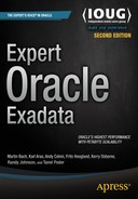
There are many optimizations that can be summarized under the offloading banner. This chapter focuses on SQL statement optimizations that are implemented via Smart Scans. The major Smart Scan optimizations are column projection, predicate filtering, and storage indexes (there are of course more!). The primary goal of most of the Smart Scan optimizations is to reduce the amount of data that needs to be transmitted back to the database servers during scan execution. However, some of the optimizations also attempt to offload CPU-intensive operations—decompression, for example. We will not cover optimizations that are not related to SQL statement processing in this chapter, such as Smart File Creation and RMAN-related optimizations. Those topics will be covered in more detail elsewhere in the book. To give you a better overview of the things to come, Figure 2-1 shows the cumulative features you can see when Smart-Scanning a segment.

These features do not necessarily apply for every single query, and not necessarily in that order. Therefore, the amount of “data returned” is a moving target. As you can read in Chapter 10, the instrumentation of Smart Scans is not perfect and leaves some detail to be desired. The next sections will discuss the various optimizations found in Figure 2-1.

One very important change that is not listed in Figure 2-1 took place with Exadata 11.2.3.3.0. This change is termed Automatic Flash Caching for Table Scan Workloads and has a dramatic effect on query performance. Previously, Smart Scans would not make use of the Exadata Smart Flash Cache unless a segment was specifically marked to make use of it by changing the cell_flash_cache attribute set to KEEP to the storage clause of the segment. This served two main purposes: First, the amount of Flash Cache was not abundant in earlier Exadata generations and, secondly, the available space was better used for OLTP-style workloads where small, single block I/O dominates. In more recent Exadata generations, there is a lot more Flash Cache available; the capacity doubles with every new generation. Currently, the X5-2 high-capacity storage server feature 4 x 1.6TB F160 Flash cards attached via NVMe to the PCIe bus. The X5-2 high-performance storage server is the first one to only have PCIe Flash cards and no spinning disk.

In the following sections, we have occasionally used performance information to prove a point. Please do not let that confuse you. Chapters 10–12 will explain these in much more detail than we can provide here. When discussing offloading, the authors sometimes face the dreaded chicken-and-egg problem. On the other hand, it is not possible to write a 100-page chapter to include all the content that might be relevant, either. Please feel free to flip between this chapter and the performance chapters just mentioned, or simply take the performance counters as additional and, hopefully, useful insights.

Column Projection

The term column projection refers to Exadata’s ability to limit the volume of data transferred between the storage tier and the database tier by only returning columns of interest. That is, those in the select list are necessary for join operations on the database tier. If your query requests five columns from a 100-column table, Exadata can eliminate most of the data that would be returned to the database servers by non-Exadata storage. This feature is a much bigger deal than you might expect, and it can have a very significant impact on response times. Here is an example:

SQL> alter session set "_serial_direct_read" = always;

Session altered.

Elapsed: 00:00:00.00
SQL> alter session set cell_offload_processing = false;

Session altered.

Elapsed: 00:00:00.00
SQL> select count(distinct seller) from sales;

COUNT(DISTINCTSELLER)
---------------------
                 1000

Elapsed: 00:00:53.55
SQL> alter session set cell_offload_processing = true;

Session altered.

Elapsed: 00:00:00.01
SQL> select count(distinct seller) from sales;

COUNT(DISTINCTSELLER)
---------------------
                 1000

Elapsed: 00:00:28.84

This example deserves some discussion. To force direct path reads—a prerequisite for Smart Scans—the session parameter _SERIAL_DIRECT_READ is set to ALWAYS (more on that later). Next, Smart Scans are explicitly disabled by setting CELL_OFFLOAD_PROCESSING to FALSE. You can see that the test query does not have a WHERE clause. This, too, is done deliberately. It means that predicate filtering and storage indexes cannot be used to cut down the volume of data that must be transferred from the storage tier because those two optimizations can only be done when there is a WHERE clause. That leaves column projection as the only optimization in play. Are you surprised that column projection alone could cut a query’s response time in half? We were the first time we saw it, but it makes sense if you think about it. And, in this particular case, the table only has 12 columns!

SQL> @desc sh.sales
           Name                            Null?        Type
           ------------------------------- --------     --------------
    1      PROD_ID                         NOT NULL     NUMBER
    2      CUST_ID                         NOT NULL     NUMBER
    3      TIME_ID                         NOT NULL     DATE
    4      CHANNEL_ID                      NOT NULL     NUMBER
    5      PROMO_ID                        NOT NULL     NUMBER
    6      QUANTITY_SOLD                   NOT NULL     NUMBER(10,2)
    7      SELLER                          NOT NULL     NUMBER(6)
    8      FULFILLMENT_CENTER              NOT NULL     NUMBER(6)
    9      COURIER_ORG                     NOT NULL     NUMBER(6)
   10      TAX_COUNTRY                     NOT NULL     VARCHAR2(3)
   11      TAX_REGION                                   VARCHAR2(3)
   12      AMOUNT_SOLD                     NOT NULL     NUMBER(10,2)

You should be aware that columns in the select list are not the only columns that must be returned to the database server. This is a very common misconception. Join columns in the WHERE clause must also be returned. As a matter of fact, in early versions of Exadata, the column projection feature was not as effective as it could have been and actually returned all the columns included in the WHERE clause, which, in many cases, included some unnecessary columns.

The DBMS_XPLAN package can display information about column projection, although by default it does not. The projection data is stored in the PROJECTION column in the V$SQL_PLAN view as well. Here is an example:

SQL> select /*+ gather_plan_statistics */
  2   count(s.prod_id), avg(amount_sold)
  3  from sales_nonpart s, products p
  4  where p.prod_id = s.prod_id
  5  and s.time_id = DATE '2013-12-01'
  6  and s.tax_country = 'DE';

COUNT(S.PROD_ID) AVG(AMOUNT_SOLD)
---------------- ----------------
             124       51.5241935

Elapsed: 00:00:00.09
SQL> select * from table(dbms_xplan.display_cursor(null,null,'+projection'));

PLAN_TABLE_OUTPUT
-------------------------------------
SQL_ID  69y720khfvjq4, child number 1
-------------------------------------
select /*+ gather_plan_statistics */  count(s.prod_id),
avg(amount_sold) from sales_nonpart s, products p where p.prod_id =
s.prod_id and s.time_id = DATE '2013-12-01' and s.tax_country = 'DE'

Plan hash value: 754104813

--------------------------------------------------------------------------------------------
| Id  | Operation                   | Name         | Rows  | Bytes | Cost (%CPU)| Time     |
--------------------------------------------------------------------------------------------
|   0 | SELECT STATEMENT            |              |       |       |  198K (100)|          |
|   1 |  SORT AGGREGATE             |              |     1 |    22 |            |          |
|*  2 |   HASH JOIN                 |              |   149 |  3278 |   198K  (2)| 00:00:08 |
|   3 |    TABLE ACCESS STORAGE FULL| PRODUCTS     |    72 |   288 |     3   (0)| 00:00:01 |
|*  4 |    TABLE ACCESS STORAGE FULL| SALES_NONPART|   229 |  4122 |   198K  (2)| 00:00:08 |
--------------------------------------------------------------------------------------------

Predicate Information (identified by operation id):
---------------------------------------------------

   2 - access("P"."PROD_ID"="S"."PROD_ID")
   4 - storage(("S"."TIME_ID"=TO_DATE(' 2013-12-01 00:00:00', 'syyyy-mm-dd
              hh24:mi:ss') AND "S"."TAX_COUNTRY"='DE'))
       filter(("S"."TIME_ID"=TO_DATE(' 2013-12-01 00:00:00', 'syyyy-mm-dd
              hh24:mi:ss') AND "S"."TAX_COUNTRY"='DE'))

Column Projection Information (identified by operation id):
-----------------------------------------------------------

   1 - (#keys=0) COUNT(*)[22], SUM("AMOUNT_SOLD")[22]
   2 - (#keys=1; rowset=200) "AMOUNT_SOLD"[NUMBER,22]
   3 - (rowset=200) "P"."PROD_ID"[NUMBER,22]
   4 - (rowset=200) "S"."PROD_ID"[NUMBER,22], "AMOUNT_SOLD"[NUMBER,22]

Note
-----
   - statistics feedback used for this statement

39 rows selected.

SQL> select projection from v$sql_plan
  2  where projection is not null
  3  and sql_id = '69y720khfvjq4'
  4  and child_number = 1;

PROJECTION
----------------------------------------------------------------
(#keys=0) COUNT(*)[22], SUM("AMOUNT_SOLD")[22]
(#keys=1; rowset=200) "AMOUNT_SOLD"[NUMBER,22]
(rowset=200) "P"."PROD_ID"[NUMBER,22]
(rowset=200) "S"."PROD_ID"[NUMBER,22], "AMOUNT_SOLD"[NUMBER,22]

Elapsed: 00:00:00.00

As you can see, the plan output shows the projection information, but only if you use the +PROJECTION argument in the call to the DBMS_XPLAN package. Note also that the PROD_ID columns from both tables are listed in the PROJECTION section, but that not all columns in the WHERE clause are included. This becomes very apparent in the predicate output for operation ID 4. Although the query narrows the result set down by specifying TIME_ID and TAX_COUNTRY, these columns are not found anywhere in the PROJECTION. Only those columns that need to be returned to the database should be listed. Note also that the projection information is not unique to Exadata, but is a generic part of the database code.

The V$SQL family of views contain columns that define the volume of data that may be saved by offloading (IO_CELL_OFFLOAD_ELIGIBLE_BYTES) and the volume of data that was actually returned by the storage servers (IO_INTERCONNECT_BYTES, IO_CELL_OFFLOAD_RETURNED_BYTES). Note that these columns are cumulative for all the executions of the statement. These columns in V$SQL will be used heavily throughout the book because they are key indicators of offload processing. Here is a quick demonstration to show that projection does affect the amount of data returned to the database servers and that selecting fewer columns results in less data transferred:

SQL> select /* single-col-test */ avg(prod_id) from sales;

AVG(PROD_ID)
------------
  80.0035113

Elapsed: 00:00:14.12
SQL> select /* multi-col-test */ avg(prod_id), sum(cust_id), sum(channel_id) from sales;

AVG(PROD_ID) SUM(CUST_ID) SUM(CHANNEL_ID)
------------ ------------ ---------------
  80.0035113   4.7901E+15      1354989738

Elapsed: 00:00:25.89
SQL> select sql_id, sql_text from v$sql where regexp_like(sql_text,'(single|multi)-col-test'),

SQL_ID        SQL_TEXT
------------- ----------------------------------------
8m5zmxka24vyk select /* multi-col-test */ avg(prod_id)
0563r8vdy9t2y select /* single-col-test */ avg(prod_id

SQL> select SQL_ID, IO_CELL_OFFLOAD_ELIGIBLE_BYTES eligible,
  2  IO_INTERCONNECT_BYTES actual,
  3  100*(IO_CELL_OFFLOAD_ELIGIBLE_BYTES-IO_INTERCONNECT_BYTES)
  4  /IO_CELL_OFFLOAD_ELIGIBLE_BYTES "IO_SAVED_%", sql_text
  5  from v$sql where SQL_ID in ('8m5zmxka24vyk', '0563r8vdy9t2y'),

SQL_ID          ELIGIBLE     ACTUAL IO_SAVED_% SQL_TEXT
------------- ---------- ---------- ---------- ----------------------------------------
8m5zmxka24vyk 1.6272E+10 4760099744 70.7475353 select /* multi-col-test */ avg(prod_id)
0563r8vdy9t2y 1.6272E+10 3108328256 80.8982443 select /* single-col-test */ avg(prod_id

SQL> @fsx4
Enter value for sql_text: %col-test%
Enter value for sql_id:

SQL_ID       CHILD OFFLOAD IO_SAVED_%  AVG_ETIME SQL_TEXT
------------- ------ ------- ---------- ---------- ----------------------------------------
0563r8vdy9t2y       0 Yes      80.90      14.11 select /* single-col-test */ avg(prod_id
8m5zmxka24vyk       0 Yes      70.75      25.89 select /* multi-col-test */ avg(prod_id)

Note that the extra columns resulted in extra time required to complete the query and that the columns in V$SQL verified the increased volume of data that had to be transferred. You could also get the first glimpse at the output of a modified version of the fsx.sql script, which will be discussed in more detail later in this chapter. For now, please just accept that it shows us whether a statement was offloaded or not.

Predicate Filtering

The second of the big three Smart Scan optimizations is predicate filtering. This term refers to Exadata’s ability to return only rows of interest to the database tier. Since the iDB protocol used to interact with the Exadata storage cells includes the predicate information in its requests, predicate filtering is accomplished by performing the standard filtering operations at the storage level before returning the data. On databases using non-Exadata storage, filtering is always done on the database servers. This generally means that a large number of records that will eventually be discarded will be returned to the database tier. Filtering these rows at the storage layer can provide a very significant decrease in the volume of data that must be transferred to the database tier. While this optimization also results in some savings in CPU usage on the database servers, the biggest advantage is generally the reduction in time needed for the data transfer.

Here is an example:

SQL> alter session set cell_offload_processing=false;

Session altered.

Elapsed: 00:00:00.01
SQL> select count(*) from sales;

  COUNT(*)
----------
 294575180

Elapsed: 00:00:23.17
SQL> alter session set cell_offload_processing=true;

Session altered.

Elapsed: 00:00:00.00
SQL> select count(*) from sales;

  COUNT(*)
----------
 294575180

Elapsed: 00:00:05.68
SQL> -- disable storage indexes
SQL> alter session set "_kcfis_storageidx_disabled"=true;

System altered.

Elapsed: 00:00:00.12
SQL> select count(*) from sales where quantity_sold = 1;

  COUNT(*)
----------
   3006298

Elapsed: 00:00:02.78

First, offloading is completely disabled using the CELL_OFFLOAD_PROCESSING parameter followed by an execution of a query without a WHERE clause (“predicate”). Without the benefit of offloading, but with the benefits of reading exclusively from Smart Flash Cache, this query took about 23 seconds. Here is proof that the data came exclusively from Smart Flash Cache, using the mystats script you will find detailed in Chapter 11. In this case, the “optimized” keyword indicates Flash Cache usage:

STAT    cell flash cache read hits                    51,483
...
STAT    physical read IO requests                     51,483
STAT    physical read bytes                   16,364,175,360
STAT    physical read requests optimized              51,483
STAT    physical read total IO requests               51,483
STAT    physical read total bytes             16,364,175,360
STAT    physical read total bytes optimized   16,364,175,360

Next, offloading is enabled, and the same query is re-executed. This time, the elapsed time was only about six seconds. The savings of approximately 18 seconds was due strictly to column projection (because without a WHERE clause for filtering, there were no other optimizations that could come into play). Using a trick to disable storage indexes by setting the hidden parameter, _KCFIS_STORAGEIDX_DISABLED, to TRUE (more in the next section) and by adding a WHERE clause, the execution time was reduced to about two seconds. This reduction of an additional three seconds or so was thanks to predicate filtering. Note that storage indexes had to be disabled in the example to make sure the query performance improvement was entirely due to the predicate filtering without other performance enhancements (that is, storage indexes) interfering.

Storage Indexes and Zone Maps

Storage indexes provide the third level of optimization for Smart Scans. Storage indexes are in-memory structures on the storage cells that maintain a maximum and minimum value for each 1MB disk storage unit, for up to eight columns of a table. They are created and maintained transparently on the cells after segments have been queried. Storage indexes are a little different than most Smart Scan optimizations. The goal of storage indexes is not to reduce the amount of data being transferred back to the database tier. In fact, whether they are used on a given query or not, the amount of data returned to the database tier remains constant. On the contrary, storage indexes are designed to eliminate time spent reading data from disk on the storage servers themselves. Think of this feature as a pre-filter. Since Smart Scans pass the query predicates to the storage servers and storage indexes contain a map of minimum and maximum values for up to eight columns in each 1MB storage region, any region that cannot possibly contain a matching row because it lies outside of the minimum and maximum value stored in the storage index can be eliminated without ever being read. You can also think of storage indexes as an alternate partitioning mechanism. Disk I/O is eliminated in analogous fashion to partition elimination. If a partition cannot contain any records of interest, the partition’s blocks will not be read. Similarly, if a storage region cannot contain any records of interest, that storage region need not be read.

Storage indexes cannot be used in all cases, and there is little that can be done to affect when or how they are used. But, in the right situations, the results from this optimization technique can be astounding. As always, this is best shown with an example:

SQL> -- disable storage indexes
SQL> alter session set "_kcfis_storageidx_disabled"=true;

System altered.

Elapsed: 00:00:00.11
SQL> select count(*) from bigtab where id = 8000000;

  COUNT(*)
----------
        32

Elapsed: 00:00:22.02
SQL> -- re-enable storage indexes
SQL> alter session set "_kcfis_storageidx_disabled"=false;

System altered.

Elapsed: 00:00:00.01
SQL> select count(*) from bigtab where id = 8000000;

  COUNT(*)
----------
        32

Elapsed: 00:00:00.54

In this example, storage indexes have again been disabled deliberately using the aforementioned parameter _KCFIS_STORAGEIDX_DISABLED to remind you of the elapsed time required to read through all rows using column projection and predicate filtering only. Remember that even though the amount of data returned to the database tier is extremely small in this case, the storage servers still had to read through every block containing data for the BIGTAB table and then had to check each row to see if it matched the WHERE clause. This is where the majority of the 22 seconds was spent. After storage indexes were re-enabled and the query was re-executed, the execution time was reduced to about .05 seconds. This reduction in elapsed time is a result of storage indexes being used to avoid virtually all the disk I/O and the time spent filtering through those records.

Beginning with Exadata version 12.1.2.1.0 and database 12.1.0.2, Oracle introduced the ability to keep overall minimum and maximum values of the minimum and maximum values of a column stored in the storage indexes in the storage server. The idea is that the min() and max() functions can pick up the overall kept value and not visit the storage indexes to compute this value. This should benefit queries using min() and max() functions such as analytical workloads where dashboards are populated with these. Unfortunately, there is no extra instrumentation available at the time of writing to indicate the cached minimum or maximum value has been used. All you can see is a change in the well-known statistic “cell physical IO bytes saved by storage index.”

Just to reiterate, column projection and predicate filtering (and most other Smart Scan optimizations) improve performance by reducing the volume of data being transferred back to the database servers (and thus the amount of time to transfer the data). Storage indexes improve performance by eliminating time spent reading data from disk on the storage servers and filtering that data. Storage indexes are covered in much more detail in Chapter 4.

Zone maps are new with Oracle 12.1.0.2 and conceptually similar to storage indexes. The difference is that a zone map grants the user more control over segments to be monitored. When we first heard about zone maps, we were very excited because the feature could have been seen as a port of the storage index (which requires an Exadata storage cell) to a non-Exadata platform. Unfortunately, the usage of zone maps is limited to Exadata, making it far less attractive. A zone in the Oracle parlance is an area of a table on disk, typically around 1024 blocks. Just as with a storage index, a zone map allows Oracle to skip areas on disk that are not relevant for a query. The big difference between zone maps and the storage indexes just discussed is that the latter are maintained on the storage servers, whereas zone maps are created and maintained under the control of the database administrator on the database level. Storage indexes reside on the cells, and the DBA has little control over them. A zone map is very similar to a materialized view, but without the need of a materialized view log. When you create a zone map, you need to decide how it is refreshed to prevent it from becoming stale. Zone-map information is also available in the database’s dictionary. When a zone map is available and can be used, you will see it applied as a filter in the execution plan.

SQL> -- turning off storage indexes as they might interfere with the result otherwise
SQL> alter session set "_kcfis_storageidx_disabled" = true;

Session altered.

Elapsed: 00:00:00.00
SQL> select /*+ gather_plan_statistics zmap_example_001 */ count(*)
  2  from T1_ORDER_BY_ID where id = 121;

  COUNT(*)
----------
        16

Elapsed: 00:00:02.65
SQL> select * from table(dbms_xplan.display_cursor);

PLAN_TABLE_OUTPUT
-------------------------------------
SQL_ID  avt7474pb4m1m, child number 0
-------------------------------------
select /*+ gather_plan_statistics zmap_example_001 */ count(*) from
T1_ORDER_BY_ID where id = 121

Plan hash value: 775109614

--------------------------------------------------------------------------------------
| Id  | Operation                      | Name           | Rows  | Bytes | Cost (%CPU)|
--------------------------------------------------------------------------------------
|   0 | SELECT STATEMENT               |                |       |       |   723K(100)|
|   1 |  SORT AGGREGATE                |                |     1 |     5 |            |
|*  2 |   TABLE ACCESS STORAGE FULL    |                |       |       |            |
|     |    WITH ZONEMAP                | T1_ORDER_BY_ID |    16 |    80 |   723K  (1)|
--------------------------------------------------------------------------------------

Predicate Information (identified by operation id):
---------------------------------------------------

   2 - storage("ID"=121)
       filter((SYS_ZMAP_FILTER('/* ZM_PRUNING */ SELECT "ZONE_ID$", CASE WHEN
              BITAND(zm."ZONE_STATE$",1)=1 THEN 1 ELSE
              CASE WHEN (zm."MIN_1_ID" > :1 OR zm."MAX_1_ID" < :2)
              THEN 3 ELSE 2 END END FROM "MARTIN"."T1_ORDER_BY_ID_ZMAP" zm
              WHERE zm."ZONE_LEVEL$"=0 ORDER BY
              zm."ZONE_ID$"',SYS_OP_ZONE_ID(ROWID),121,121)<3 AND "ID"=121))

24 rows selected.

When you look at the SQL traces for the statement, you will see that the zone maps are consulted for extends eligible for pruning in recursive SQL statements executed as SYS. The traced statements look just like the filter reported in the execution plan.

Simple Joins (Bloom Filters)

In some cases, join processing can be offloaded to the storage tier as well. Offloaded joins are accomplished by creating what is called a Bloom filter. Bloom filters have been around for a long time and have been used by Oracle since Oracle Database Version 10g Release 2. Hence, they are not specific to Exadata. One of the main ways Oracle uses them is to reduce traffic between parallel query slaves. As of Oracle 11.2.0.4 and 12c, you can also have Bloom filters in serial query processing.

Bloom filters have the advantage of being very small relative to the data set that they represent. However, this comes at a price—they can return false positives. That is, rows that should not be included in the desired result set can occasionally pass a Bloom filter. For that reason, an additional filter must be applied after the Bloom filter to ensure that any false positives are eliminated. An interesting fact about Bloom filters from an Exadata perspective is that they may be passed to the storage servers and evaluated there, effectively transforming a join to a filter. This technique can result in a large decrease in the volume of data that must be transmitted back to database servers. The following example demonstrates this:

SQL> show parameter bloom

PARAMETER_NAME                       TYPE        VALUE
----------------------------------- ----------- ------
_bloom_predicate_offload             boolean     FALSE

SQL> show parameter kcfis

PARAMETER_NAME                       TYPE        VALUE
----------------------------------- ----------- ------
_kcfis_storageidx_disabled            boolean     TRUE

SQL> select /* bloom0015 */ * from customers c, orders o
  2  where o.customer_id = c.customer_id and c.cust_email = '[email protected]';

no rows selected

Elapsed: 00:00:13.57
SQL> alter session set "_bloom_predicate_offload" = true;

Session altered.

SQL> select /* bloom0015 */ * from customers c, orders o
  2  where o.customer_id = c.customer_id and c.cust_email = '[email protected]';

no rows selected

Elapsed: 00:00:02.56
SQL> @fsx
Enter value for sql_text: %bloom0015%
Enter value for sql_id:

SQL_ID         CHILD  PLAN_HASH  EXECS  AVG_ETIME AVG_PX OFFLOAD IO_SAVED_% SQL_TEXT
------------- ------ ---------- ------ ---------- ------ ------- ---------- --------------
5n3np45j2x9vn      0  576684111      1      13.56      0 Yes          54.26 select /* bloom0015
5n3np45j2x9vn      1 2651416178      1       2.56      0 Yes          99.98 select /* bloom0015

SQL> --fetch first explain plan, without bloom filter
SQL> select * from table(
  2   dbms_xplan.display_cursor('5n3np45j2x9vn',0,'BASIC +predicate +partition'));

PLAN_TABLE_OUTPUT
------------------------
EXPLAINED SQL STATEMENT:
------------------------
select /* bloom0015 */ * from customers c, orders o where o.customer_id
= c.customer_id and c.cust_email = '[email protected]'

Plan hash value: 576684111

-----------------------------------------------------------------
| Id  | Operation                   | Name      | Pstart| Pstop |
-----------------------------------------------------------------
|   0 | SELECT STATEMENT            |           |       |       |
|*  1 |  HASH JOIN                  |           |       |       |
|   2 |   PARTITION HASH ALL        |           |     1 |    32 |
|*  3 |    TABLE ACCESS STORAGE FULL| CUSTOMERS |     1 |    32 |
|   4 |   PARTITION HASH ALL        |           |     1 |    32 |
|   5 |    TABLE ACCESS STORAGE FULL| ORDERS    |     1 |    32 |
-----------------------------------------------------------------

Predicate Information (identified by operation id):
---------------------------------------------------

   1 - access("O"."CUSTOMER_ID"="C"."CUSTOMER_ID")
   3 - storage("C"."CUST_EMAIL"='[email protected]')
       filter("C"."CUST_EMAIL"='[email protected]')

25 rows selected.

Elapsed: 00:00:00.01
SQL> --fetch second explain plan, with bloom filter
SQL> select * from table(
  2  dbms_xplan.display_cursor('5n3np45j2x9vn',1,'BASIC +predicate +partition'));

PLAN_TABLE_OUTPUT
------------------------
EXPLAINED SQL STATEMENT:
------------------------
select /* bloom0015 */ * from customers c, orders o where o.customer_id
= c.customer_id and c.cust_email = '[email protected]'

Plan hash value: 2651416178

------------------------------------------------------------------
| Id  | Operation                    | Name      | Pstart| Pstop |
------------------------------------------------------------------
|   0 | SELECT STATEMENT             |           |       |       |
|*  1 |  HASH JOIN                   |           |       |       |
|   2 |   JOIN FILTER CREATE         | :BF0000   |       |       |
|   3 |    PARTITION HASH ALL        |           |     1 |    32 |
|*  4 |     TABLE ACCESS STORAGE FULL| CUSTOMERS |     1 |    32 |
|   5 |   JOIN FILTER USE            | :BF0000   |       |       |
|   6 |    PARTITION HASH ALL        |           |     1 |    32 |
|*  7 |     TABLE ACCESS STORAGE FULL| ORDERS    |     1 |    32 |
------------------------------------------------------------------

Predicate Information (identified by operation id):
---------------------------------------------------

   1 - access("O"."CUSTOMER_ID"="C"."CUSTOMER_ID")
   4 - storage("C"."CUST_EMAIL"='[email protected]')
       filter("C"."CUST_EMAIL"='[email protected]')
   7 - storage(SYS_OP_BLOOM_FILTER(:BF0000,"O"."CUSTOMER_ID"))
       filter(SYS_OP_BLOOM_FILTER(:BF0000,"O"."CUSTOMER_ID"))

29 rows selected.

In this listing, the hidden parameter, _BLOOM_PREDICATE_OFFLOAD (previously in 11.2 it was named _BLOOM_PREDICATE_PUSHDOWN_TO_STORAGE), was used for comparison purposes. Notice that the test query ran in about 2 seconds with Bloom filters, and 14 seconds without. Also notice that both queries were offloaded. If you look closely at the predicate information of the plans, you will see that the SYS_OP_BLOOM_FILTER(:BF0000,"O"."CUSTOMER_ID") predicate was run on the storage servers for the second run, indicated by child cursor 1. The query that used Bloom filters ran faster because the storage servers were able to pre-join the tables, which eliminated a large amount of data that would otherwise have been transferred back to the database servers. The Oracle database engine is not limited to using a single Bloom filter, depending on the complexity of the query there can be more.

Function Offloading

Oracle’s implementation of the Structured Query Language (SQL) includes many built-in functions. These functions can be used directly in SQL statements. Broadly speaking, they may be divided into two main groups: single-row functions and multi-row functions. Single-row functions return a single result row for every row of a queried table. These single-row functions can be further subdivided into the following general categories:

• Numeric functions (SIN, COS, FLOOR, MOD, LOG, ...)
• Character functions (CHR, LPAD, REPLACE, TRIM, UPPER, LENGTH, ...)
• Datetime functions (ADD_MONTHS, TO_CHAR, TRUNC, ...)
• Conversion functions (CAST, HEXTORAW, TO_CHAR, TO_DATE, ...)

Virtually all of these single-row functions can be offloaded to Exadata storage. The second major group of SQL functions operate on a set of rows. There are two subgroups in this multi-row function category:

• Aggregate functions (AVG, COUNT, SUM, ...)
• Analytic functions (AVG, COUNT, DENSE_RANK, LAG, ...)

These functions return either a single row (aggregate functions) or multiple rows (analytic functions). Note that some of the functions are overloaded and belong to both groups. None of these functions can be offloaded to Exadata, which makes sense because many of these functions require access to the entire set of rows—something individual storage cells do not have.

There are some additional functions that do not fall neatly into any of the previously described groupings. These functions may or may not be offloaded to the storage cells. For example, DECODE and NVL are offloadable, but most XML functions are not. Some of the data mining functions are offloadable, but some are not. Also keep in mind that the list of offloadable functions may change as newer versions are released. The definitive list of offloadable functions for your particular version is contained in V$SQLFN_METADATA. In 11.2.0.3, for example, 393 out of 923 SQL functions 393 were offloadable.

SQL> select count(*), offloadable from v$sqlfn_metadata group by rollup(offloadable);

   COUNT(*) OFF
----------- ---
        530 NO
        393 YES
        923

In 12.1.0.2, the current release at the time of writing, the number of functions increased:

SQL> select count(*), offloadable from v$sqlfn_metadata group by rollup(offloadable);

  COUNT(*) OFF
---------- ---
       615 NO
       418 YES
      1033

Offloading functions does allow the storage cells to do some of the work that would normally be done by the CPUs on the database servers. However, the saving in CPU usage is generally a relatively minor enhancement. The big gain usually comes from limiting the amount of data transferred back to the database servers. Being able to evaluate functions contained in WHERE clauses allows storage cells to send only rows of interest back to the database tier. So, as with most offloading, the primary goal of this optimization is to reduce the amount of traffic between the storage and database tiers. If a function has been offloaded to the storage servers, you can see this in the predicate section emitted by DBMS_XPLAN.DISPLAY_CURSOR, as shown here:

SQL> select count(*) from sales where lower(tax_country) = 'ir';

  COUNT(*)
----------
    435700

SQL> select * from table(dbms_xplan.display_cursor(null, null, 'BASIC +predicate'));

PLAN_TABLE_OUTPUT
------------------------
EXPLAINED SQL STATEMENT:
------------------------
select count(*) from sales where lower(tax_country) = 'ir'

Plan hash value: 3519235612

---------------------------------------------
| Id  | Operation                   | Name  |
---------------------------------------------
|   0 | SELECT STATEMENT            |       |
|   1 |  SORT AGGREGATE             |       |
|   2 |   PARTITION RANGE ALL       |       |
|*  3 |    TABLE ACCESS STORAGE FULL| SALES |
---------------------------------------------

Predicate Information (identified by operation id):
---------------------------------------------------

   3 - storage(LOWER("TAX_COUNTRY")='ir')
       filter(LOWER("TAX_COUNTRY")='ir')

This is not to be confused with referencing a function in the select-list:

SQL> select lower(tax_country) from sales where rownum < 11;

LOW
---
zl
uw
...
bg

10 rows selected.

SQL> select * from table(dbms_xplan.display_cursor(null, null, 'BASIC +predicate'));

PLAN_TABLE_OUTPUT
------------------------
EXPLAINED SQL STATEMENT:
------------------------
select lower(tax_country) from sales where rownum < 11

Plan hash value: 807288713

--------------------------------------------------------
| Id  | Operation                              | Name  |
--------------------------------------------------------
|   0 | SELECT STATEMENT                       |       |
|*  1 |  COUNT STOPKEY                         |       |
|   2 |   PARTITION RANGE ALL                  |       |
|   3 |    TABLE ACCESS STORAGE FULL FIRST ROWS| SALES |
--------------------------------------------------------

Predicate Information (identified by operation id):
---------------------------------------------------

   1 - filter(ROWNUM<11)

As you can see, there is no reference to the to_lower() function in the predicate information. You will, however, benefit from column projection in this case.

Compression/Decompression

One Exadata feature that has received quite a bit of attention is HCC. Exadata offloads the decompression of data stored in HCC format during Smart Scan operations. That is, columns of interest are decompressed on the storage cells when the compressed data is accessed via Smart Scans. This decompression is not necessary for filtering, so only the data that will be returned to the database tier will be decompressed. Note that all compression is done at the database tier, however. Decompression may also be done at the database tier when data is not accessed via a Smart Scan or when the storage cells are very busy. To make it simple, Table 2-1 shows where the work is done.

Decompressing data at the storage tier runs counter to the theme of most of the other Smart Scan optimizations. Most of them are geared to reducing the volume of data to be transported back to the database servers. Because decompression is such a CPU-intensive task, particularly with the higher levels of compression, the decision was made to do the decompression on the storage servers whenever possible. This decision is not set in stone, however, as in some situations there may be ample CPU resources available to make decompressing data on the database servers an attractive option. (That is, in some situations, the reduction in data to be shipped may outweigh the reduction in database-server CPU consumption.) In fact, as of cellsrv version 11.2.2.3.1, Exadata does have the ability to return compressed data to the database servers when the storage cells are busy. Chapter 3 deals with HCC in much more detail and will provide examples for such situations.

There is a hidden parameter that controls whether decompression will be offloaded at all. Unfortunately, it does not just move the decompression back and forth between the storage and database tiers. If the _CELL_OFFLOAD_HYBRIDCOLUMNAR parameter is set to a value of FALSE, Smart Scans will be completely disabled on HCC data.

Encryption/Decryption

Encryption and decryption are handled in a manner very similar to compression and decompression of HCC data. Encryption is always done at the database tier, while decryption can be done by the storage servers or by the database servers. When encrypted data is accessed via Smart Scan, it is decrypted on the storage servers. Otherwise, it is decrypted on the database servers. Note that from the X2 Exadata generation, Intel Xeon chips in the storage servers have built-in capabilities to perform cryptography in silicon. Modern Intel chips contain a special instruction set (Intel AES-NI) that effectively adds a hardware boost to processes doing encryption or decryption. Note that Oracle Database Release 11.2.0.2 or later is necessary to take advantage of the new instruction set.

Encryption and HCC compression work well together. Since compression is done first, there is less work needed for processes doing encryption and decryption on HCC data. Note that the CELL_OFFLOAD_DECRYPTION parameter controls this behavior, and that as it does with the hidden parameter _CELL_OFFLOAD_HYBRIDCOLUMNAR, setting the parameter to a value of FALSE completely disables Smart Scans on encrypted data, which also disables decryption at the storage layer.

Virtual Columns

Virtual columns provide the ability to define pseudo-columns that can be calculated from other columns in a table, without actually storing the calculated value. Virtual columns may be used as partition keys, used in constraints, or indexed. Column level statistics can also be gathered on them. Since the values of virtual columns are not actually stored, they must be calculated on the fly when they are accessed. Outside the Exadata platform, the database session has to calculate the values. On Exadata, these calculations can be offloaded for a segment access via Smart Scans:

SQL> alter table bigtab add idn1 generated always as (id + n1);

Table altered.

SQL> select column_name, data_type, data_default
  2  from user_tab_columns where table_name = 'BIGTAB';

COLUMN_NAME          DATA_TYPE            DATA_DEFAULT
-------------------- -------------------- ------------
IDN1                 NUMBER               "ID"+"N1"
ID                   NUMBER
V1                   VARCHAR2
N1                   NUMBER
N2                   NUMBER
N_256K               NUMBER
N_128K               NUMBER
N_8K                 NUMBER
PADDING              VARCHAR2

9 rows selected.

Now you can query the table including the virtual column. To demonstrate the effect of offloading, a random value is needed first. The combination of ID and N1 should be reasonably unique in this data set:

SQL> select /*+ gather_plan_statistics virtual001 */ id, n1, idn1 from bigtab where rownum < 11;

        ID         N1       IDN1
---------- ---------- ----------
   1161826       1826    1163652
   1161827       1827    1163654
   1161828       1828    1163656
   1161829       1829    1163658
   1161830       1830    1163660
   1161831       1831    1163662
   1161832       1832    1163664
   1161833       1833    1163666
   1161834       1834    1163668
   1161835       1835    1163670

10 rows selected.

Here is the demonstration of how the offloaded calculation benefits the execution time:

SQL> select /* gather_plan_statistics virtual0002 */ count(*)
  2  from bigtab where idn1 = 1163652;

  COUNT(*)
----------
        64

Elapsed: 00:00:06.78
SQL> @fsx4
Enter value for sql_text: %virtual0002%
Enter value for sql_id:

SQL_ID         CHILD OFFLOAD IO_SAVED_%  AVG_ETIME SQL_TEXT
------------- ------ ------- ---------- ---------- ----------------------------------------
8dyyd6kzycztq      0 Yes          99.99       6.77 select /* virtual0002 */ count(*) from b

Elapsed: 00:00:00.39
SQL> @dplan
Copy and paste SQL_ID and CHILD_NO from results above
Enter value for sql_id: 8dyyd6kzycztq
Enter value for child_no:

PLAN_TABLE_OUTPUT
-------------------------------------
SQL_ID  8dyyd6kzycztq, child number 0
-------------------------------------
select /* virtual0002 */ count(*) from bigtab where idn1 = 1163652

Plan hash value: 2140185107

-------------------------------------------------------------------------------------
| Id  | Operation                  | Name   | Rows  | Bytes | Cost (%CPU)| Time     |
-------------------------------------------------------------------------------------
|   0 | SELECT STATEMENT           |        |       |       |  2780K(100)|          |
|   1 |  SORT AGGREGATE            |        |     1 |    13 |            |          |
|*  2 |   TABLE ACCESS STORAGE FULL| BIGTAB |  2560K|    31M|  2780K  (1)| 00:01:49 |
-------------------------------------------------------------------------------------

Predicate Information (identified by operation id):
---------------------------------------------------

   2 - storage("ID"+"N1"=1163652)
       filter("ID"+"N1"=1163652)

The amount of I/O saved is 99.99%, as calculated using the quintessential columns in V$SQL for the last execution, and the query took 6.78 seconds to finish.

As with so many features in the Oracle world, there is a parameter to influence the behavior of your session. In the next example, the relevant underscore parameter will be used to disable virtual column processing at the storage server level. This is done to simulate how the same query would run on a non-Exadata platform:

SQL> alter session set "_cell_offload_virtual_columns"=false;

Session altered.

Elapsed: 00:00:00.00
SQL> select /* virtual0002 */ count(*)
  2  from bigtab where idn1 = 1163652;

  COUNT(*)
----------
        64

Elapsed: 00:00:23.13

The execution time is visibly higher when the compute nodes have to evaluate the expression. Comparing the two statement’s execution shows this:

SQL> @fsx4
Enter value for sql_text: %virtual0002%
Enter value for sql_id:

SQL_ID         CHILD OFFLOAD IO_SAVED_%  AVG_ETIME SQL_TEXT
------------- ------ ------- ---------- ---------- ----------------------------------------
8dyyd6kzycztq      0 Yes          99.99       6.77 select /* virtual0002 */ count(*) from b
8dyyd6kzycztq      1 Yes          94.18      23.13 select /* virtual0002 */ count(*) from b

2 rows selected.

You will also note the absence of the storage keyword in the predicates section when displaying the execution plan for the first child cursor:

SQL> @dplan
Copy and paste SQL_ID and CHILD_NO from results above
Enter value for sql_id: 8dyyd6kzycztq
Enter value for child_no: 1

PLAN_TABLE_OUTPUT
-------------------------------------
SQL_ID  8dyyd6kzycztq, child number 1
-------------------------------------
select /* virtual0002 */ count(*) from bigtab where idn1 = 1163652

Plan hash value: 2140185107

-------------------------------------------------------------------------------------
| Id  | Operation                  | Name   | Rows  | Bytes | Cost (%CPU)| Time     |
-------------------------------------------------------------------------------------
|   0 | SELECT STATEMENT           |        |       |       |  2780K(100)|          |
|   1 |  SORT AGGREGATE            |        |     1 |    13 |            |          |
|*  2 |   TABLE ACCESS STORAGE FULL| BIGTAB |    64 |   832 |  2780K  (1)| 00:01:49 |
-------------------------------------------------------------------------------------

Predicate Information (identified by operation id):
---------------------------------------------------

   2 - filter("ID"+"N1"=1163652)

Note
-----
   - statistics feedback used for this statement

If you are using virtual columns in WHERE clauses, you certainly get a benefit from the Exadata platform.

Support for LOB offloading

With the introduction of Exadata software 12.1.1.1.1 and RDBMS 12.1.0.2, queries against inline LOBs defined as SecureFiles can be offloaded as well. According to the documentation set, like and regexp_like can be offloaded. To demonstrate this new feature, a new table, LOBOFFLOAD ,has been created and populated with 16 million rows. This should ensure that it is considered for Smart Scans. Here is the crucial bit of information about the LOB column:

SQL> select table_name, column_name, segment_name, securefile, in_row
  2  from user_lobs where table_name = 'LOBOFFLOAD';

TABLE_NAME              COLUMN_NAME             SEGMENT_NAME                  SEC IN_
---------------------   ---------------------   ---------------------------   --- ---
LOBOFFLOAD              COMMENTS                SYS_LOB0000096135C00002$$     YES YES

The table tries to model a common application technique where a CLOB has been defined in a table to enter additional, unstructured information related to a record. This should be OK as long as it does not circumvent the constraints in the data model and purely informational information is stored that is not needed for processing in any form. Here is the example in 12c:

SQL> select /*+ monitor loboffload001 */ count(*) from loboffload where comments like '%GOOD%';

  COUNT(*)
----------
     15840

Elapsed: 00:00:02.93


SQL> @fsx4.sql
Enter value for sql_text: %loboffload001%
Enter value for sql_id:


SQL_ID         CHILD OFFLOAD IO_SAVED_%  AVG_ETIME SQL_TEXT
------------- ------ ------- ---------- ---------- -----------------------------------------
18479dnagkkyu      0 Yes          98.94       2.93 select /*+ monitor loboffload001 */ count

As you can see in the output of the script (which we will discuss in more detail later), the query is offloaded. This is not the case in 11.2.0.3 where the test case has been reproduced:

SQL> select /*+ monitor loboffload001 */ count(*) from loboffload where comments like '%GOOD%';

   COUNT(*)
-----------
      15840
Elapsed: 00:01:34.04

SQL> @fsx4.sql
Enter value for sql_text: %loboffload001%
Enter value for sql_id:

SQL_ID         CHILD OFFLOAD IO_SAVED_%  AVG_ETIME SQL_TEXT
------------- ------ ------- ---------- ---------- -----------------------------------------
18479dnagkkyu      0 No             .00      94.04 select /*+ monitor loboffload001 */ count

Unlike in the first example, the second query executed on 11.2.0.3 was not offloaded. Due to the segment size, it used direct path reads, but, unlike in the first example, they did not turn into Smart Scans.

JSON Support and Offloading

With the introduction of Oracle 12.1.0.2, JSON support was added to the database layer. If you are on Exadata 12.1.0.2.1.0 or later, you can benefit from offloading some of these operators. As you saw in the section about function offloading, you can query v$sqlfn_metadata about a function’s ability to be offloaded. Here is the result when checking for JSON-related functions and their offloading support:

SQL> select count(*), name, offloadable from v$sqlfn_metadata
  2  where name like '%JSON%' group by name, offloadable
  3  order by offloadable, name;

  COUNT(*) NAME                           OFF
---------- ------------------------------ ---
         1 JSON_ARRAY                     NO
         1 JSON_ARRAYAGG                  NO
         1 JSON_EQUAL                     NO
         1 JSON_OBJECT                    NO
         1 JSON_OBJECTAGG                 NO
         1 JSON_QUERY                     NO
         1 JSON_SERIALIZE                 NO
         1 JSON_TEXTCONTAINS2             NO
         1 JSON_VALUE                     NO
         2 JSON                           YES
         1 JSON_EXISTS                    YES
         1 JSON_QUERY                     YES
         1 JSON_VALUE                     YES

13 rows selected.

Users of 12.1.0.2.1 also benefit from the ability to offload XMLExists and XMLCast operations as per the Oracle documentation.

Data Mining Model Scoring

Some of the data model scoring functions can be offloaded. Generally speaking, this optimization is aimed at reducing the amount of data transferred to the database tier as opposed to pure CPU offloading. As with other function offloading, you can verify which data mining functions can be offloaded by querying V$SQLFN_METADATA. The output looks like this:

SQL> select distinct name, version, offloadable
  2  from V$SQLFN_METADATA
  3  where name like 'PREDICT%'
  4  order by 1,2
  5  /

NAME                           VERSION      OFF
------------------------------ ------------ ---
PREDICTION                     V10R2 Oracle YES
PREDICTION_BOUNDS              V11R1 Oracle NO
PREDICTION_COST                V10R2 Oracle YES
PREDICTION_DETAILS             V10R2 Oracle NO
PREDICTION_PROBABILITY         V10R2 Oracle YES
PREDICTION_SET                 V10R2 Oracle NO

6 rows selected.

As you can see, some of the functions are offloadable, and some are not. The ones that are offloadable can be used by the storage cells for predicate filtering. Here’s an example query that should only return records that meet the scoring requirement specified in the WHERE clause:

SQL> select cust_id
  2  from customers
  3  where region = 'US'
  4  and prediction_probability(churnmod,'Y' using *) > 0.8
  5  /

This optimization is designed to offload CPU usage as well as reduce the volume of data transferred. However, it is most beneficial in situations where it can reduce the data returned to the database tier, such as in the previous example.

Non-Smart Scan Offloading

There are a few optimizations that are not related to query processing. As these are not the focus of this chapter, we will only touch on them briefly.

Smart/Fast File Creation

This optimization has a somewhat misleading name. It really is an optimization designed to speed up block initialization. Whenever blocks are allocated, the database must initialize them. This activity happens when tablespaces are created, but it also occurs when files are added or extended for any number of other reasons. On non-Exadata storage, these situations require the database server to format each block and then write it back to disk. All that reading and writing causes a lot of traffic between the database servers and the storage cells. As you are now aware, eliminating traffic between the layers is a primary goal of Exadata. As you might imagine, this totally unnecessary traffic has been eliminated.

This process has been further refined. Beginning with Oracle Exadata 11.2.3.3.0 (a hot contender for the authors’ favorite Exadata release), Oracle introduced fast data file creation. The time it takes to initialize a data file can be further reduced by using a clever trick. The first optimization you read about in the previous paragraph was to delegate the task of zeroing out the data files to the cells, which in itself proves quite effective. The next logical step, and what you get with fast file creation, is to just write the metadata to the Write-Back Flash Cache (WBFC), thus eliminating the actual process of formatting the blocks. If WBFC is enabled in the cell, the fast data file creation will be used by default. You can read more about Exadata Smart Flash Cache in Chapter 5.

RMAN Incremental Backups

Exadata speeds up incremental backups by increasing the granularity of block change tracking. On non-Exadata platforms, block changes are tracked for groups of blocks; on Exadata, changes are tracked for individual blocks. This can significantly decrease the number of blocks that must be backed up, resulting in smaller backup sizes, less I/O bandwidth, and reduced time to complete incremental backups. This feature can be disabled by setting the _DISABLE_CELL_OPTIMIZED_BACKUPS parameter to a value of TRUE. This optimization is covered in Chapter 10 in more detail.

RMAN Restores

This optimization speeds up the file initialization portion when restoring from backup on a cell. Although restoring databases from backups is not very common, this optimization can also help speed up cloning of environments. The optimization reduces CPU usage on the database servers and reduces traffic between the two tiers. If the _CELL_FAST_FILE_RESTORE parameter is set to a value of FALSE, this behavior will be disabled. This optimization is also covered in Chapter 10.

Smart Scan Prerequisites

Smart Scans do not occur for every query run on Exadata. There are three basic requirements that must be met for Smart Scans to occur:

• There must be a full scan of a segment (table, partition, materialized view, and so forth).
• The scan must use Oracle’s direct path read mechanism.
• The object must be stored on Exadata storage.

There is a simple explanation as to why these requirements exist. Oracle is a C program. The function that performs Smart Scans (kcfis_read) is called by the direct path read function (kcbldrget), which is called by one of the full scan functions. It’s that simple. You can’t get to the kcfis_read function without traversing the code path from full scan to direct read. And, of course, the storage will have to be running Oracle’s software in order to process Smart Scans with all data files residing on Exadata. We will discuss each of these requirements in turn.

Full Scans

In order for queries to take advantage of Exadata’s offloading capabilities, the optimizer must decide to execute a statement with a full table scan or a fast full index scan. These terms are used somewhat generically in this context. A full segment scan is a prerequisite for direct path reads as well. As you just read, there will not be a Smart Scan unless there is a direct path read decision made.

Generally speaking, the (fast) full scan corresponds to TABLE ACCESS FULL and INDEX FAST FULL SCAN operations of an execution plan. With Exadata, these familiar operations have been renamed slightly to show that they are accessing Exadata storage. The new operation names are TABLE ACCESS STORAGE FULL and INDEX STORAGE FAST FULL SCAN.

It is usually quite simple to work out if a full scan has happened, but you might need to look in more than one place. The easiest way to start your investigation is to call DBMS_XPLAN.DISPLAY_CURSOR() right after a query has finished executing:

SQL> select count(*) from bigtab;

  COUNT(*)
----------
 256000000

Elapsed: 00:00:07.98

SQL> select * from table(dbms_xplan.display_cursor(null, null));

PLAN_TABLE_OUTPUT
-------------------------------------
SQL_ID  8c9rzdry8yahs, child number 0
-------------------------------------
select count(*) from bigtab

Plan hash value: 2140185107

-----------------------------------------------------------------------------
| Id  | Operation                  | Name   | Rows  | Cost (%CPU)| Time     |
-----------------------------------------------------------------------------
|   0 | SELECT STATEMENT           |        |       |  2779K(100)|          |
|   1 |  SORT AGGREGATE            |        |     1 |            |          |
|   2 |   TABLE ACCESS STORAGE FULL| BIGTAB |   256M|  2779K  (1)| 00:01:49 |
-----------------------------------------------------------------------------

Alternatively, you can use the fsx.sql script to locate the SQL text of a query from the shared pool and invoke the DISPLAY_CURSOR() function with the SQL_ID and cursor child number. The dplan.sql script is a convenient way to do so.

Note that there are also some minor variations of these operations, such as MAT_VIEW ACCESS STORAGE FULL, that also qualify for Smart Scans of materialized views. You should, however, be aware that the fact that your execution plan shows a TABLE ACCESS STORAGE FULL operation does not mean that your query was performed with a Smart Scan. It merely means that this particular prerequisite has been satisfied. Later in the chapter, you will read about methods on how to verify whether a statement was actually offloaded via a Smart Scan.

Direct Path Reads

In addition to requiring full scan operations, Smart Scans also require that the read operations be executed via Oracle’s direct path read mechanism. Direct path reads have been around for a long time. Traditionally, this read mechanism has been used by parallel query server processes. Because parallel queries were originally expected to be used for accessing very large amounts of data (typically much too large to fit in the Oracle buffer cache), it was decided that the parallel servers should read data directly into their own memory (also known as the program global area or PGA). The direct path read mechanism completely bypasses the standard Oracle caching mechanism of placing blocks in the buffer cache. It relies on the fast object checkpoint operation to flush dirty buffers to disk before “scooping” them up in multi-block reads. This was a very good thing for very large data sets, as it eliminated extra work that was not expected to be helpful (caching full table scan data that would probably not be reused) and kept them from flushing other data out of the cache. Additionally, the inherent latency of random seeks in hard disks was eliminated. Not inserting buffers read in the buffer cache also removes a lot of potential CPU overhead.

This was the state of play until Oracle 11g, where non-parallel queries started to use direct path reads as well. This was a bit of a surprise at the time!

As a direct consequence, Smart Scans do not require parallel execution. The introduction of the direct path reads for serial queries certainly benefits the Exadata way of reading data by means of Smart Scan. You read previously that the kcfis (kernel cache file intelligent storage) functions are buried under the kcbldrget (kernel cache block direct read get) function. Therefore, Smart Scans can only be performed if the direct path read mechanism is being used.

Serial queries do not always use Smart Scans—that would be terribly inefficient. Setting up a direct path read, especially in clustered environments, can be a time-consuming task. Therefore, direct path reads are only set up and used when the conditions are right.

A hidden parameter, _SERIAL_DIRECT_READ, controls this feature. When this parameter is set to its default value (AUTO), Oracle automatically determines whether to use direct path reads for non-parallel scans. The calculation is based on several factors including the size of the object, the size of the buffer cache, and the number of the object’s blocks are already cached in the buffer cache. There is also a hidden parameter (_SMALL_TABLE_THRESHOLD) that plays a role in determining how big a table must be before it will be considered for serial direct path reads. The algorithm for determining whether to use the direct path read mechanism on non-parallel scans is not published. With a little digging, you can excavate some of the decision-making process. In recent versions of the database, you can trace a RDBMS kernel facility named NSMTIO. The low-level oradebug utility can be invoked to display traceable components in the database, and one top-level component is named KXD—Exadata specific kernel modules (kxd):

SQL> oradebug doc component kxd

KXD                        Exadata specific Kernel modules (kxd)
KXDAM                      Exadata Disk Auto Manage (kxdam)
KCFIS                      Exadata Predicate Push (kcfis)
NSMTIO                     Trace Non Smart I/O (nsmtio)
KXDBIO                     Exadata Block level Intelligent Operations (kxdbio)
KXDRS                      Exadata Resilvering Layer (kxdrs)
KXDOFL                     Exadata Offload (kxdofl)
KXDMISC                    Exadata Misc (kxdmisc)
KXDCM                      Exadata Metrics Fixed Table Callbacks (kxdcm)
KXDBC                      Exadata Backup Compression for Backup Appliance (kxdbc)

Tracing KXD.* is quite interesting from a research point of view, but it should never be done outside a lab environment due to the potentially large size trace files it generates. The NSMTIO subcomponent has interesting information about the direct path read decision. The first trace shown here is about a direct path read that turned into a Smart Scan:

SQL> select value from v$diag_info
  2  where name like 'Default%';

VALUE
------------------------------------------------------------------/u01/app/oracle/diag/rdbms/dbm01/dbm011/trace/dbm011_ora_32020.trc

SQL> alter session set events 'trace[nsmtio]';

Session altered.

Elapsed: 00:00:00.00
SQL> select count(*) from bigtab;

  COUNT(*)
----------
 256000000

Elapsed: 00:00:08.10
SQL> !cat /u01/app/oracle/diag/rdbms/dbm01/dbm011/trace/dbm011_ora_32020.trc
NSMTIO: kcbism: islarge 1 next 0 nblks 10250504 type 3, bpid 65535, kcbisdbfc 0 kcbnhl
   262144 kcbstt 44648 keep_nb 0 kcbnbh 2232432 kcbnwp 3
NSMTIO: kcbism: islarge 1 next 0 nblks 10250504 type 2, bpid 3, kcbisdbfc 0 kcbnhl 262144
  kcbstt 44648 keep_nb 0 kcbnbh 2232432 kcbnwp 3
NSMTIO: kcbimd: nblks 10250504 kcbstt 44648 kcbpnb 223243 kcbisdbfc 3 is_medium 0
NSMTIO: kcbivlo: nblks 10250504 vlot 500 pnb 2232432 kcbisdbfc 0 is_large 0
NSMTIO: qertbFetch:[MTT < OBJECT_SIZE < VLOT]:
  Checking cost to read from caches(local/remote) and checking storage reduction factors
  (OLTP/EHCC Comp)
NSMTIO: kcbdpc:DirectRead: tsn: 7, objd: 34422, objn: 20491
ckpt: 1, nblks: 10250504, ntcache: 2173249, ntdist:2173249
Direct Path for pdb 0 tsn 7  objd 34422 objn 20491
Direct Path 1 ckpt 1, nblks 10250504 ntcache 2173249 ntdist 2173249
Direct Path mndb 0 tdiob 6 txiob 0 tciob 43
Direct path diomrc 128 dios 2 kcbisdbfc 0
NSMTIO: Additional Info: VLOT=11162160
Object# = 34422, Object_Size = 10250504 blocks
SqlId = 8c9rzdry8yahs, plan_hash_value = 2140185107, Partition# = 0

BIGTAB is relatively large at 10250504 blocks. Earlier releases of the Exadata software performed a single-block read of the segment header to determine the object size. Since 11.2.0.2, the hidden parameter _direct_read_decision_statistics_driven is set to TRUE, implying that the dictionary statistics will be consulted instead. 2173249 blocks are cached in the buffer cache, which does not seem to play a role here. However, if too many blocks are cached, a buffered access path can be chosen instead of a direct path read.

The table access function (qertbFetch) reports that the object is larger than the MTT or medium table threshold and smaller than the VLOT or very large object threshold. Thankfully, the SQL_ID and plan hash value of the statement in question are shown here, as is the partition.

Unfortunately, the medium table threshold is a bit misleading in the interval definition [MTT < OBJECT_SIZE < VLOT]. The MTT is calculated as five times the _small_table_threshold (STT), and on first glance seems to be the cut-off point from where a direct path read is considered. This is probably true for early 11.2 releases. A test in 11.2.0.3 and later, including 12c, shows that segments can be eligible for direct path reads even when they are just a bit larger than the STT. The decision is then based on the number of blocks in the buffer cache (remote and local are considered in RAC) and their type. This is indicated in the trace by the line “checking cost to read from caches (local/remote) and checking storage reduction factors...”.

On the other hand, if there is no direct path read, you will see something like this for a really small table:

NSMTIO: kcbism: islarge 0 next 0 nblks 4 type 3, bpid 65535, kcbisdbfc 0 kcbnhl 262144
  kcbstt 48117 keep_nb 0 kcbnbh 2405898 kcbnwp 3
NSMTIO: kcbism: islarge 0 next 0 nblks 4 type 2, bpid 3, kcbisdbfc 0 kcbnhl 262144 kcbstt 48117
  keep_nb 0 kcbnbh 2405898 kcbnwp 3
NSMTIO: qertbFetch:NoDirectRead:[- STT < OBJECT_SIZE < MTT]:Obect's size: 4 (blocks), Threshold:
  MTT(240589 blocks),
_object_statistics: enabled, Sage: enabled,
Direct Read for serial qry: enabled(::::kctfsage::), Ascending SCN table scan: FALSE
flashback_table_scan: FALSE, Row Versions Query: FALSE
SqlId: 71acyavyyg1dg, plan_hash_value: 2604480108, Object#: 25576, Parition#: 0
  DW_scan: disabled

In this trace, you can see that the object is far too small—only four blocks. No direct path read was chosen since the segment is smaller than the _small_table_threshold. The last argument of the trace is interesting as well: A DW_SCAN is related to the Automatic Big Table Caching (ABTC), which has nothing to do with offloading queries to the storage servers.

There is another case that could be identified. It is related to the VLOT, or very large object threshold. You could see a reference in the first NSMTIO listing, where BIGTAB was smaller than that threshold. The VLOT defaults to 500, or five times the size of the buffer cache. The additional information provided in the first NSMTIO trace reveals that the VLOT is 11162160. The instance’s buffer cache is approximately 20GB in size, or 2232432 buffers. The current number of buffers in the instance’s buffer cache can be retrieved from v$db_cache_advise as so:

SQL> select block_size,size_for_estimate,buffers_for_estimate
  2  from v$db_cache_advice where size_factor = 1 and name = 'DEFAULT';

BLOCK_SIZE SIZE_FOR_ESTIMATE BUFFERS_FOR_ESTIMATE
---------- ----------------- --------------------
      8192             20608              2232432

Multiplying 2232432 by 5 returns 11162160; remember that db_block_buffers are measured as blocks and not bytes.

While the ability to do serial direct path reads has been around for some time, it has only become a relatively common occurrence since Oracle 11g. Oracle Database 11gR2 has a modified version of the calculations used to determine whether to use direct path reads for non-parallel scans. The new modifications to the algorithm make the direct path read mechanism much more likely to occur than it was in previous versions. This was probably done as a result of Exadata’s Smart Scan optimizations and the desire for them to be triggered whenever possible. The algorithm may be somewhat overly aggressive on non-Exadata platforms.

Exadata Storage

Of course, the data being scanned must be stored on Exadata storage in order for Smart Scans to occur. It is possible to create ASM disk groups that access non-Exadata storage on Exadata database servers. And, of course, it makes sense that any SQL statements accessing objects defined using these non-Exadata disk groups will not be eligible for offloading.

While it is unusual, it is also possible to create ASM disk groups using a combination of Exadata and non-Exadata storage. Since you cannot put Fibre Channel Host Bus Adaptors into an Exadata compute node, this leaves network-attached storage the only option. With the introduction of NAS solutions, such as the ZFS Storage Appliance, it is increasingly common to move colder data to cheaper storage, accessed via dNFS. We cover this scenario in Chapter 3 in the context of the Automatic Data Optimization (ADO).

Queries against objects whose segments reside on mixed storage are not eligible for offloading. There is actually an attribute assigned to ASM disk groups (cell.smart_scan_capable) that specifies whether a disk group is capable of processing Smart Scans. This attribute must be set to FALSE before non-Exadata storage can be assigned to an ASM disk group.

The dictionary view DBA_TABLESPACES ha a property, named PREDICATE_EVALUATION, that you can query, too. This is the output from a query against our X4-2 half-rack lab database:

SQL> select tablespace_name, bigfile, predicate_evaluation
  2  from dba_tablespaces;

TABLESPACE_NAME                BIG PREDICA
------------------------------ --- -------
SYSTEM                         NO  STORAGE
SYSAUX                         NO  STORAGE
UNDOTBS1                       YES STORAGE
TEMP                           YES STORAGE
UNDOTBS2                       YES STORAGE
UNDOTBS3                       YES STORAGE
UNDOTBS4                       YES STORAGE
USERS                          NO  STORAGE
SOE                            YES STORAGE
SH                             YES STORAGE

Smart Scan Disablers

There are situations where Smart Scans are effectively disabled. The simple case is where they have not been enabled in the code yet, so Smart Scans cannot happen at all. There are other cases where Oracle starts down the Smart Scan path, but the storage software either decides, or is forced, to revert to block shipping mode. Generally, this decision is made on a block-by-block basis. The complete list of Smart Scan disablers is found in the Exadata documentation set, which, fortunately, was publicly available at the time of writing. Refer to Chapter 7 of the Storage Server Software User’s Guide, section “Using the SQL EXPLAIN PLAN Command with Oracle Exadata Storage Server Software.” You might want to refer to it from time to time as Oracle continuously enhances the software, and current restrictions may be lifted in future releases.

Simply Unavailable

During the discussion of Smart Scan optimizations, you read about the prerequisites that must be met to enable Smart Scans. However, even when those conditions are met, there are circumstances that prevent Smart Scans. Here are a few other situations that are not related to specific optimizations, but where Smart Scans simply cannot be used:

• On clustered tables or Index Organized Tables (IOTs)
• The query scans out-of-line LOB or LONG data types
• On tables with ROWDEPENDENCIES enabled
• Instances when you query features a flashback_query_clause
• Instances when you cannot offload queries against reverse key indexes
• Instances when you are querying data on non-Exadata storage

You also saw some parameters in the previous sections that influence Smart Scan behavior. If you set CELL_OFFLOAD_PROCESSING to FALSE or maybe _SERIAL_DIRECT_READ to never, you cannot by definition have Smart Scans.

Reverting to Block Shipping

There are situations where Smart Scans are used, but for various reasons cellsrv reverts to block shipping mode. This is a very complex topic, and we struggled with whether to include it in an introductory chapter on offloading. But since it is a fundamental concept, we decided to discuss it here, albeit briefly. There is a lot more detail about this subject in Chapter 11.

So far, Smart Scans have been described in this chapter as a means to avoid transferring large amounts of data to the database layer by returning pre-filtered data directly to the PGA. The brunt of the work is carried out by the storage cells—the more there are, the faster the scan can be performed. Just because your query is returning only 2% of the table data does not mean that you can avoid scanning all of it, as you can see in V$SQL and some other places you will learn more about in this book. Remember that the storage cells operate completely independently of one another; in other words, they do not communicate during query processing, ever. Communication during query processing is limited to the information exchange between the storage servers and the compute node (or multiple nodes if you process a query in parallel across the cluster). Another important piece of information in this context is that Smart Scans will only return consistent reads, not current blocks.

Occasionally, Smart Scans can choose (or be forced) to return complete blocks to the SGA. Basically, any situation that would cause Oracle to have to read another block to complete/roll back a record to the snapshot SCN will cause this to happen. A chained row is another, and perhaps the simplest, example. When Oracle encounters a chained row, the row’s headpiece will contain a pointer to the block containing the second row piece. Since the storage cells do not communicate directly with each other and it is unlikely that the chained block resides on the same storage cell, cellsrv simply ships the entire block and allows the database layer to deal with it.

In this very simple case, the Smart Scan is paused momentarily, and a single-block read is effectively performed, which motivates another single-block read to get the additional row piece. Keep in mind that this is a very simple case.

This same behavior comes into play when Oracle must deal with read consistency issues. For example, if Oracle notices that a block is “newer” than the current query’s SCN, the process of finding an age-appropriate version of the block is left for the database layer to deal with. This effectively pauses the Smart Scan processing while the database does its traditional read consistency processing. Delayed block cleanout is a similar case that might require pausing a Smart Scan.

So, is this really important, and why should you care? The answer, of course, is that it depends. In most cases, you probably do not need to be concerned. Oracle guarantees that reads will be consistent, even when doing Smart Scans. Several optimizations, such as the commit cache discussed in Chapter 11, help speed up processing. The fact that Oracle behaves exactly the same from the application standpoint, regardless of whether Smart Scans are used or not, is a big deal. Exadata is not a highly specialized analytical engine. It is still using exactly the same database software everyone else does. The fact that Oracle may do some single-block reads along with its Smart Scan is of little concern if the results are correct and the performance is not severely impacted, and in most cases it will not be. There are cases, though, where choosing to do a Smart Scan and then reverting to block shipping mode can be painful from a performance standpoint. These are the cases where it is important to understand what is going on under the covers. Again, you can find more information on this issue in Chapter 11.

Skipping Some Offloading

Another very complex behavior that we will only mention briefly is the ability of cellsrv to refuse to do some of the normal offload processing. This can be done to avoid overloading the CPU resources on the storage cells, for example. A good example of this behavior occurs when decompressing HCC data. Decompression is an extremely CPU-intensive task, especially for the higher levels of compression. Since Exadata storage software 11.2.2.3.0 and later, cellsrv can choose to skip the decompression step on some portion of the data when the CPUs on the storage cells are very busy. This effectively moves some of the workload back to the database tier by forcing the database hosts to do the decompression.

Skipping Offloading silently

Sometimes the Exadata software has to revert to what is called passthrough mode. This can be a source of concern since it is not always evident this has happened, especially in 11g Release 2. The problem is best explained with an example. The following query normally takes very little time to execute:

SQL> select count(*) from bigtab where id = 80000;

  COUNT(*)
----------
        32

Elapsed: 00:00:00.83

Assume that the statement suddenly takes 25 seconds to execute. The systematic approach would be to check for changed plans, statistics, data volume, and so on. But nothing changed (this time for real). The statement was offloaded to the storage cells when it executed in less than a second, and checking now you can see that the wait event is indicating offloading, too. If you have the licenses to use ASH, you could use a very basic query like this one to that effect:

SQL> select count(*), event, session_state from v$active_session_history
  2  where sql_id = '0pmmwn5xq8h9a' group by event, session_state;

  COUNT(*) EVENT                        SESSION
---------- ---------------------------- -------
        28                               ON CPU
        46 cell smart table scan        WAITING

Interestingly, the query is offloaded, as you can see in the presence of the Cell Smart Table Scan event. The solution to the question, “Why is it slow?,” must be elsewhere. At the risk of getting a little bit ahead of us, it lies in the session statistics. Using the tools snapper or mystats described in Chapter 11, you can find out that there are lots of passthrough operations:

Type    Statistic Name                                                               Value
------  ----------------------------------------------------------------  ----------------
STAT    cell num bytes in passthru during predicate offload                 28,004,319,232
STAT    cell num smart IO sessions using passthru mode due to cellsrv                    1
STAT    cell physical IO bytes eligible for predicate offload               83,886,137,344
STAT    cell physical IO bytes saved by storage index                       51,698,524,160
STAT    cell physical IO interconnect bytes returned by smart scan          28,004,930,160

Passthrough mode implies that the cells still perform a part of the Smart Scan, but instead of applying the predicate filtering, they pass the entire block to the RDBMS layer. You can read more about passthrough mode in Chapter 11.

How to Verify That Smart Scan Is Happening

One of the most important things you can learn about Exadata is how to identify whether a query has been able to take advantage of Smart Scans. Interestingly, the normal execution plan output produced by the DBMS_XPLAN package will not show you whether a Smart Scan was used or not. Here’s an example:

PLAN_TABLE_OUTPUT
-------------------------------------
SQL_ID  2y17pb7bnmpt0, child number 0
-------------------------------------
select count(*) from bigtab where id = 17000

Plan hash value: 2140185107

-------------------------------------------------------------------------------------
| Id  | Operation                  | Name   | Rows  | Bytes | Cost (%CPU)| Time     |
-------------------------------------------------------------------------------------
|   0 | SELECT STATEMENT           |        |       |       |  2779K(100)|          |
|   1 |  SORT AGGREGATE            |        |     1 |     6 |            |          |
|*  2 |   TABLE ACCESS STORAGE FULL| BIGTAB |    32 |   192 |  2779K  (1)| 00:01:49 |
-------------------------------------------------------------------------------------

Predicate Information (identified by operation id):
---------------------------------------------------

   2 - storage("ID"=17000)
       filter("ID"=17000)

Notice that the optimizer chose a TABLE ACCESS STORAGE FULL operation and that the predicate section shows a storage() predicate associated with step 2 of the plan. Both of these characteristics indicate that a Smart Scan was possible, but neither provides a definitive verification. In fact, the statement in this listing was not executed with a Smart Scan. If you wonder why, we set _serial_direct_read to never in the session just prior to executing the query.

The fact that execution plans do not show whether a Smart Scan was performed is a bit frustrating. However, there are several techniques that you can use to work around this issue. The next few sections will introduce some useful techniques. Note that the topic of analyzing whether a Smart Scan happened and how effective it was is covered in much more detail in Chapters 10 and 11.

10046 Trace

One of the most straightforward ways to determine whether a Smart Scan was used is to enable a 10046 trace on the statement in question. Unfortunately, this is a bit cumbersome and does not allow you to do any investigation into what has happened with past executions. Nevertheless, tracing is a fairly foolproof way to verify whether a Smart Scan was used or not. If a Smart Scan was used, there will be CELL SMART TABLE SCAN or CELL SMART INDEX SCAN events in the trace file. Here is an excerpt from the trace file collected for the previous statement (reformatted for better readability):

PARSING IN CURSOR #1..4 len=44 dep=0 uid=65 oct=3 lid=65 tim=1625363834946
  hv=3611940640 ad='5e7a2e420' sqlid='2y17pb7bnmpt0'
WAIT #139856525281664: nam='cell single block physical read' ela= 1237 ...
WAIT #139856525281664: nam='cell single block physical read' ela= 651 ...
WAIT #139856525281664: nam='cell single block physical read' ela= 598 ...
...
WAIT #139856525281664: nam='cell multiblock physical read' ela= 1189 ...
WAIT #139856525281664: nam='cell single block physical read' ela= 552 ...
WAIT #139856525281664: nam='cell multiblock physical read' ela= 596 ...
WAIT #139856525281664: nam='cell multiblock physical read' ela= 612 ...
WAIT #139856525281664: nam='cell multiblock physical read' ela= 607 ...
WAIT #139856525281664: nam='cell multiblock physical read' ela= 632 ...
WAIT #139856525281664: nam='cell multiblock physical read' ela= 618 ...
[...]

Note that the events recorded in this part of the trace file are single-block and multi-block reads. Oracle used the opportunity to rename the db file sequential read and db file scattered read wait events to the less confusing cell single-block read and cell multi-block read. Here’s an example showing a Smart Scan:

PARSING IN CURSOR #139856525283104 len=44 dep=0 uid=65 oct=3 lid=65 tim=1625653524727
  hv=3611940640 ad='5e7a2e420' sqlid='2y17pb7bnmpt0'
select count(*) from bigtab where id = 17000
END OF STMT
PARSE #139856525283104:c=0,e=117,p=0,cr=0,cu=0,mis=0,r=0,dep=0,og=1,plh=2140185107,...
EXEC #139856525283104:c=0,e=55,p=0,cr=0,cu=0,mis=0,r=0,dep=0,og=1,plh=2140185107,...
WAIT #139856525283104: nam='SQL*Net message to client' ela= 3 ...
WAIT #139856525283104: nam='reliable message' ela= 1049 channel context=26855200120 ...
WAIT #139856525283104: nam='enq: KO - fast object checkpoint' ela= 298 ...
WAIT #139856525283104: nam='enq: KO - fast object checkpoint' ela= 156 ...
WAIT #139856525283104: nam='cell smart table scan' ela= 151 ...
WAIT #139856525283104: nam='cell smart table scan' ela= 168 ...
WAIT #139856525283104: nam='cell smart table scan' ela= 153 ...
WAIT #139856525283104: nam='cell smart table scan' ela= 269 ...
WAIT #139856525283104: nam='cell smart table scan' ela= 209 ...
WAIT #139856525283104: nam='cell smart table scan' ela= 231 ...
WAIT #139856525283104: nam='cell smart table scan' ela= 9 ...
[...]

In the second example, you can see many cell Smart Table Scan events, indicating that processing has been offloaded to the storage tier.

Session Performance Statistics

Another possibility is to look at some of the performance views such as V$SESSSTAT and V$MYSTAT. This is often overlooked but very helpful as you saw in the section about passthrough mode. An excellent way to investigate what is happening with a session that is currently executing a SQL statement is Tanel Poder’s Snapper script. It provides a great way to see what wait events are being generated while a statement is running. In addition, it can capture the change in session counters during the period the SQL statement is observed. Snapper focuses on actively executing SQL statements; it is not meant to go back in time.

Performance statistics provide a reliable source of data as long as you can access the system during the execution of the statement you are investigating. Here is an example using V$MYSTATS, which is simply a version of V$SESSSTAT that limits data to your current session. For this example, the focus is on the cell scans statistic, which is incremented when a Smart Table Scan occurs on a segment:

SQL> @mystat
Enter value for name: cell scans

NAME                       VALUE
--------------------------------
cell scans                     0

Elapsed: 00:00:00.04
SQL> select count(*) from bigtab where id = 17001;

  COUNT(*)
----------
        32

Elapsed: 00:00:00.44
SQL> @mystat
Enter value for name: cell scans

NAME                       VALUE
--------------------------------
cell scans                     1

Elapsed: 00:00:00.02
SQL>

As you can see, the query has triggered the incrementing of the session counter. It is safe to say that there has been a Smart Scan between the two executions of the mystats script.

There is a lot more to say about session counters, and we do so in Chapter 11.

Offload Eligible Bytes

There is another clue to whether a statement used a Smart Scan or not. As you saw in previous sections, the V$SQL family of views contain a column called IO_CELL_OFFLOAD_ELIGIBLE_BYTES, which shows the number of bytes that are eligible for offloading. This column can be used as an indicator of whether a statement used a Smart Scan. It appears that this column is set to a value greater than 0 only when a Smart Scan is used. You can make use of this observation to write a little script (fsx.sql) that returns a value of YES or NO, depending on whether that column in V$SQL has a value greater than 0. The output of the script is a little too wide to fit in a book format, which is why there are a couple of cut-down versions in the examples. And, of course, all of the versions will be available in the online code repository. You have already seen the script in action in several of the previous sections. The script is shown here for your convenience, along with an example of its use:

> !cat fsx.sql
----------------------------------------------------------------------------------------
--
-- File name:   fsx.sql
--
-- Purpose:     Find SQL and report whether it was Offloaded and % of I/O saved.
--
-- Usage:       This scripts prompts for two values.
--
--              sql_text: a piece of a SQL statement like %select col1, col2 from skew%
--
--              sql_id: the sql_id of the statement if you know it (leave blank to ignore)
--
-- Description:
--
--              This script can be used to locate statements in the shared pool and
--              determine whether they have been executed via Smart Scans.
--
--              It is based on the observation that the IO_CELL_OFFLOAD_ELIGIBLE_BYTES
--              column in V$SQL is only greater than 0 when a statement is executed
--              using a Smart Scan. The IO_SAVED_% column attempts to show the ratio of
--              of data received from the storage cells to the actual amount of data
--              that would have had to be retrieved on non-Exadata storage. Note that
--              as of 11.2.0.2, there are issues calculating this value with some queries.
--
--              Note that the AVG_ETIME will not be acurate for parallel queries. The
--              ELAPSED_TIME column contains the sum of all parallel slaves. So the
--              script divides the value by the number of PX slaves used which gives an
--              approximation.
--
--              Note also that if parallel slaves are spread across multiple nodes on
--              a RAC database the PX_SERVERS_EXECUTIONS column will not be set.
--
---------------------------------------------------------------------------------------
set pagesize 999
set lines 190
col sql_text format a70 trunc
col child format 99999
col execs format 9,999
col avg_etime format 99,999.99
col "IO_SAVED_%" format 999.99
col avg_px format 999
col offload for a7

select sql_id, child_number child, plan_hash_value plan_hash, executions execs,
(elapsed_time/1000000)/decode(nvl(executions,0),0,1,executions)/
decode(px_servers_executions,0,1,px_servers_executions/
decode(nvl(executions,0),0,1,executions)) avg_etime,
px_servers_executions/decode(nvl(executions,0),0,1,executions) avg_px,
decode(IO_CELL_OFFLOAD_ELIGIBLE_BYTES,0,'No','Yes') Offload,
decode(IO_CELL_OFFLOAD_ELIGIBLE_BYTES,0,0,
100*(IO_CELL_OFFLOAD_ELIGIBLE_BYTES-IO_INTERCONNECT_BYTES)
/decode(IO_CELL_OFFLOAD_ELIGIBLE_BYTES,0,1,IO_CELL_OFFLOAD_ELIGIBLE_BYTES))
"IO_SAVED_%", sql_text
from v$sql s
where upper(sql_text) like upper(nvl('&sql_text',sql_text))
and sql_text not like 'BEGIN :sql_text := %'
and sql_text not like '%IO_CELL_OFFLOAD_ELIGIBLE_BYTES%'
and sql_id like nvl('&sql_id',sql_id)
order by 1, 2, 3
/

In the fsx script, you can see that the OFFLOAD column is just a DECODE that checks to see if the IO_CELL_OFFLOAD_ELIGIBLE_BYTES column is equal to 0 or not. The IO_SAVED_% column is calculated using the IO_INTERCONNECT_BYTES field, and it attempts to show how much data was returned to the database servers.

The script can be used for many useful purposes. The author primarily uses it to find the SQL_ID and child cursor number of SQL statements in the shared pool. In this example, it is used to determine if a statement has been offloaded or not:

SQL> select /*+ gather_plan_statistics fsx-example-002 */
  2  avg(id) from bigtab where id between 1000 and 50000;

   AVG(ID)
----------
     25500

Elapsed: 00:00:00.64
SQL> alter session set cell_offload_processing=false;

Session altered.

Elapsed: 00:00:00.00
SQL> select /*+ gather_plan_statistics fsx-example-002 */
  2  avg(id) from bigtab where id between 1000 and 50000;

   AVG(ID)
----------
     25500

Elapsed: 00:00:53.88
SQL> @fsx4
Enter value for sql_text: %fsx-example-002%
Enter value for sql_id:

SQL_ID         CHILD OFFLOAD IO_SAVED_%  AVG_ETIME SQL_TEXT
------------- ------ ------- ---------- ---------- ----------------------------------------
cj0p52wha5wb8      0 Yes          99.97        .63 select /*+ gather_plan_statistics fsx-ex
cj0p52wha5wb8      1 No             .00      53.88 select /*+ gather_plan_statistics fsx-ex

2 rows selected.

The elapsed times are a bit of a giveaway as to whether the statement was offloaded or not, but if you are called in after the fact, the output of the fsx script clearly shows that the child_number 1 has not been offloaded. The fact that a new child cursor has been created is very important in this example. When setting CELL_OFFLOAD_PROCESSING to FALSE, the optimizer created a new child cursor due to a mismatch. Reasons why child cursors are created can be found in v$sql_shared_cursor. This view contains a long list of flags that allow you to identify differences between child cursors but is very hard to read in SQL*Plus. Oracle added a CLOB containing XML data in 11.2.0.2 that makes it easier to spot the difference. Using the SQL ID from the previous example, this is put to use. Note that I cast the CLOB to XML for better readability:

SQL> select xmltype(reason) from v$sql_shared_cursor
  2   where sql_id = 'cj0p52wha5wb8' and child_number = 0;

XMLTYPE(REASON)
---------------------------------------------------------------------------
<ChildNode>
  <ChildNumber>0</ChildNumber>
  <ID>3</ID>
  <reason>Optimizer mismatch(12)</reason>
  <size>2x356</size>
  <cell_offload_processing> true     false  </cell_offload_processing>
</ChildNode>

Translating the XML output into plain English, you can see that there was an optimizer mismatch: The parameter cell_offload_processing has changed from TRUE to FALSE.

It is not always the case for child cursors to be created after changing parameters. Certain underscore parameters such as _SERIAL_DIRECT_READ will not cause a new child cursor to be created. Some executions of the same cursor might be offloaded, others not. This can be quite confusing, although this should be a very rare occurrence! Here is an example to demonstrate the effect:

SQL> select /*+ gather_plan_statistics fsx-example-004 */ avg(id)
  2  from bigtab where id between 1000 and 50002;

   AVG(ID)
----------
     25501

Elapsed: 00:00:00.68
SQL> alter session set "_serial_direct_read" = never;

Session altered.

Elapsed: 00:00:00.00
SQL> select /*+ gather_plan_statistics fsx-example-004 */ avg(id)
  2  from bigtab where id between 1000 and 50002;

   AVG(ID)
----------
     25501

Elapsed: 00:04:50.32
SQL> SQL> alter session set "_serial_direct_read" = auto;

Session altered.

Elapsed: 00:00:00.00
SQL> select /*+ gather_plan_statistics fsx-example-004 */ avg(id)
  2  from bigtab where id between 1000 and 50002;

   AVG(ID)
----------
     25501

Elapsed: 00:00:00.63
SQL> @fsx4
Enter value for sql_text: %fsx-example-004%
Enter value for sql_id:

SQL_ID         CHILD OFFLOAD IO_SAVED_%  AVG_ETIME SQL_TEXT
------------- ------ ------- ---------- ---------- ----------------------------------------
6xh6qwv302p13      0 Yes          55.17      97.21 select /*+ gather_plan_statistics fsx-ex

As you can see, there are three executions using the same child cursor (no new child cursor has been created). The statistics about I/O saved and execution time now have little value: Two executions completed in less than a second, and one took almost five minutes. This is the well-known problem with averages: They obfuscate detail.

SQL Monitoring

There is one other tool that is very useful for determining whether a SQL statement was offloaded, which is pretty cool for all performance investigations actually. The REPORT_SQL_MONITOR procedure is part of the Real Time SQL Monitoring functionality that was added with 11g. It is built into the DBMS_SQLTUNE package and provides a great deal of information, provided you have the license to use it. Not only does it provide information whether a statement was offloaded, but also on which steps in a plan were offloaded. Here is an example of an offloaded statement. Unfortunately the output is too wide—it has been condensed a little bit, but still has the essential information:

SQL> select /*+ gather_plan_statistics monitor sqlmonexample001 */
  2  count(*) from bigtab where id between 1000 and 50000;

  COUNT(*)
----------
   1568032
Elapsed: 00:00:00.66

SQL> @report_sql_monitor
Enter value for sid:
Enter value for sql_id:
Enter value for sql_exec_id:

REPORT
------------------------------
SQL Monitoring Report

SQL Text
------------------------------
select /*+ gather_plan_statistics monitor sqlmonexample002 */ count(*) from bigtab where id between 1000 and 50000

Global Information
------------------------------
 Status              :  DONE (ALL ROWS)
 Instance ID         :  1
 Session             :  MARTIN (1108:55150)
 SQL ID              :  0kytf1zmdt5f1
 SQL Execution ID    :  16777216
 Execution Started   :  01/22/2015 05:59:26
 First Refresh Time  :  01/22/2015 05:59:26
 Last Refresh Time   :  01/22/2015 05:59:36
 Duration            :  10s
 Module/Action       :  SQL*Plus/-
 Service             :  SYS$USERS
 Program             :  [email protected] (TNS V1-V3)
 Fetch Calls         :  1

Global Stats
=========================================================================================
| Elapsed |   Cpu   |    IO    | Application | Fetch | Buffer | Read  | Read  |  Cell   |
| Time(s) | Time(s) | Waits(s) |  Waits(s)   | Calls |  Gets  | Reqs  | Bytes | Offload |
=========================================================================================
|      11 |    4.03 |     7.25 |        0.00 |     1 |    10M | 80083 |  78GB |  99.96% |
=========================================================================================

SQL Plan Monitoring Details (Plan Hash Value=2140185107)
============================================================================================
| Id |      Operation             |  Name  | Cost |   Time    | Activity | Activity Detail ||    |                            |        |      | Active(s) |   (%)    |     (# samples)

|

============================================================================================
|  0 |SELECT STATEMENT            |        |      |         9 |          |                 ||  1 | SORT AGGREGATE             |        |      |         9 |          |                 ||  2 |  TABLE ACCESS STORAGE FULL | BIGTAB |   3M |         9 |   100.00 | Cpu (3)         ||    |                            |        |      |           |          | cell smart table

|

|    |                            |        |      |           |          | scan (6)

        |

============================================================================================

You can see that the report shows a Cell Offload percentage for the entire statement in the global section. In the details section, it also shows which steps were offloaded and what they did (Activity Detail) based on ASH samples. It also shows where the statement spent its time (Activity %). This can be extremely useful with more complex statements that have multiple steps eligible for offloading. Statements that are executed in parallel have that information listed per query server process, which leads to the next point worth mentioning: The text version of the SQL Monitor report can become difficult to read for more complex statements. The most useful output format you can get is by passing ALL to REPORT_LEVEL and ACTIVE as the TYPE parameter. The resulting output is an HTML file you can open in a browser and enjoy. Oracle Enterprise Manager offers GUI access to the SQL Monitor output as well. You can learn a lot more about all aspects around SQL Monitor in Chapter 12.

Note that monitoring occurs automatically on parallelized statements and on statements that the optimizer anticipates will run for a long time. If Oracle is not automatically choosing to monitor a statement that is of interest, you can use the MONITOR hint to tell Oracle to monitor the statement, as seen in the example. You can check V$SQL_MONITOR to see if you can create a report on your SQL_ID.

Parameters

There are several parameters that apply to offloading. The main one is CELL_OFFLOAD_PROCESSING, which turns offloading on and off. There are several others that are of less importance. Table 2-2 shows a list of the non-hidden parameters that affect offloading (as of Oracle database version 12.1.0.2). Note that we have also included the hidden parameter, _SERIAL_DIRECT_READ, which controls this very important feature.

In addition to the normal Oracle-approved parameters, there are a number of so-called hidden parameters that affect various aspects of offloading. You can view them using the parms.sql script provided in the online code repository by connecting as SYSDBA and specifying both kcfis (for kernel file intelligent storage) and cell (for all cellsrv related parameters). As always, note that hidden parameters should not be used on Oracle systems without prior discussion and consent from Oracle support, but they do provide valuable clues about how some of the Exadata features work and are controlled.

Summary

Offloading really is the secret sauce of Exadata. While the hardware architecture does a good job of providing more balance between the storage layer’s ability to deliver data and the database layer’s ability to consume it, the bulk of the performance gains are provided by the software. Smart Scans are largely responsible for these gains. The primary focus of most of these optimizations is to reduce the amount of data transferred between the storage tier and the database tier. If you have read the whole chapter from beginning to end, you will undoubtedly have noticed that there is a lot of ground to cover. Where possible, we stayed with the fundamentals necessary to understand offloading. Chapters 10–11 go into a lot more detail on the various important aspects. They introduce all the relevant Exadata wait events and most of the performance counters that Oracle tracks for each session. Chapter 12 finally gives you the overview of the tools needed to analyze Exadata query performance.