
Readers of this chapter probably fall into one of three categories. They have either:
Never designed a database before
Designed a database for a transaction processing–type system
Built a data warehouse system
In the latter case, you could skip this chapter or use it as a refresher, especially if your last database used Oracle. Therefore, this chapter is aimed at readers who fall into categories one or two, which may surprise the person who has previously designed a non-data warehouse database. Why? Because the skills and techniques used to create a database for a data warehouse will be different from those required for a transaction processing–type (OLTP) system. Consequently, though you will have a head start because some of the techniques are the same, it is very important to say to yourself: I am designing a different type of database.
So what is different about designing a database in a data warehouse? In a transaction-processing system, the designer’s goal is to make the transaction complete very, very quickly, and the designer also has the benefit of hopefully knowing how the business will interrogate and use the data. Typically, the data changed is just the specific individual records for the transaction, and reports only look at the current day, month, or week. Contrast that with a data warehouse, where, although queries must complete as quickly as possible, they could still take hours. In the data warehouse, a much larger volume of data, both current and historical, is typically scanned in order to fulfill the normal business intelligence types of queries.
Another major problem is determining what information should be held in the warehouse and at what level of granularity it should be retained. This book will not discuss the techniques that can be used to determine what should be included in the warehouse or how to go about collecting that data, because there are already many books available that discuss this topic extensively.
However, the importance of trying to determine what should be included in the data warehouse cannot be stressed enough. It is so important because it may not be until a year after the warehouse is in production use that you suddenly discover that the information is either not available or held at an inappropriate level, and this will limit or prohibit the types of queries that you can run on your warehouse
For example, a telephone company decides not to hold every call in its database, but instead holds a total of what the customer spent by day. Then someone in the company decides that he or she would like to offer customers a discount when certain numbers are called. Now, if the warehouse had contained every single telephone call made by its customers, the company would be able to find out exactly what this scheme would have cost if it had been implemented over the last 12 months. Instead, it has no data available and would either have to guess what the cost might be or postpone the planned new system until sufficient data is available to accurately determine the true cost to the company.
One of the difficult decisions for the designer is to determine at what level data will be stored in the warehouse. Often, storing every transaction, such as in our telephone example, may seem rather excessive, and, because it could easily mean the warehouse grows to many terabytes, there is a temptation to consolidate the data. Managing a terabyte warehouse requires careful and stringently controlled procedures that must be followed. The bigger the database becomes, the harder it is to manage and query it. However, with the easier availability of cheap storage devices, keeping vast quantities of data at the detailed level is becoming much more feasible and worthy of serious consideration.
Since aggregation is a major design decision, the designer would be wise to seek approval from the users of the warehouse before adopting such a strategy. It should also be clearly explained to these users the limitations that are likely to occur due to aggregating the data. With disks declining in price, hopefully most sites will store all of the data that they require.
The typical approach used to construct a transaction-processing system is to construct an entity-relationship (E-R) diagram of the business. It is then ultimately used as the basis for creating the physical database design, because many of the entities in our model become tables in the database. If you have never designed a data warehouse before but are experienced in designing transaction-processing systems, then you will probably think that a data warehouse is no different from any other database and that you can use the same approach.
Unfortunately, that is not the case, and warehouse designers will quickly discover that the entity-relationship model is not really suitable for designing a data warehouse. Leading authorities on the subject, such as Ralph Kimball, advocate using the dimensional model, and we have found this approach to be ideal for a data warehouse.
An entity-relationship diagram can show us, in considerable detail, the interaction between the numerous entities in our system, removing redundancy in the system whenever possible. The result is a very flat view of the enterprise, where hundreds of entities are described along with their relationships to other entities. While this approach is fine in the transaction-processing world, where we require this level of detail, it is far too complex for the data warehouse. If you ask a database administrator (DBA) if he or she has an entity-relationship diagram, the DBA will probably respond that he or she did once, when the system was first designed. But due to its size and the numerous changes that have occurred in the system during its lifetime, the entity-relationship diagram hasn’t been updated, and it is now only partially accurate.
If we use a different approach for the data warehouse, one that results in a much simpler picture, then it should be very easy to keep it up-to-date and also to give it to end users, to help them understand the data warehouse. Another factor to consider is that entity-relationship diagrams tend to result in a normalized database design, whereas in a data warehouse, a denormalized design is often used.
An alternative to using the entity-relationship model is the dimensional model, which views and models the data from a different perspective. Instead of considering an entity, which represents a thing such as a product or a place and the relationships between those entities, a dimensional model describes data using dimensions and facts, which become actual tables in the database and which we will describe in more detail in the next two sections.
Dimensional models, as illustrated in Figure 2.1, despite sometimes looking quite simple, provide a very effective way of holding historical and current data in a form that makes it accessible to business users and that enables them to make the right business decisions. A dimensional data warehouse can be viewed as containing data that:
Has been validated (i.e., no invalid product codes)
Is historical (i.e., the last 36 months)
Is integrated—therefore the same key is used by all systems
Is easily accessible
The fact table, of which there could be more than one, contains factual information, and it is usually the largest table in the data warehouse and is often fast growing. The fact tables are typically where all of the detail data that you want to keep in the data warehouse is stored, such as all of the telephone calls made by a customer or the orders placed by your customer, as shown in Figure 2.1.
Therefore, if a customer made 20 telephone calls, then it is likely that 20 rows will be stored in the fact table for this customer. Consequently, the fact tables will be by far the largest tables in the database, possibly containing hundreds of millions of rows in a large data warehouse. If you are unsure as to whether data is factual, it is often numeric, and sometimes a value that can be computed, such as the value of an order or the number of items purchased.
The information contained in the fact table doesn’t have to be at the finest level of detail; it could be summarized data, such as total telephone calls made by a customer today. The level at which data is held in the fact table is known as the granularity and is one of the important decisions the warehouse designer must make. In the example described here, the difference in the number of records stored over a 24-month period would be huge. Contrast the storage requirements between a record stored for every telephone call a customer made in a single day compared with a record for every telephone call a customer makes.
When designing a data warehouse, depending on your business, you may find that there are different types of fact tables, such as, transaction level, transaction item level, event based, status, or even summarized data.
When designing using the dimensional model, there may only be one or a small number of fact tables, but there could be many dimension tables. The dimension table can be seen as a reference table to the fact table, where descriptions and more static information about a piece of data are held. For example, product is considered a dimension because, in this table, everything about the product is held, such as full product name, suppliers, and pallet size. In the fact table, there would be a column called “product_key,” which is used to retrieve all of the product information from this dimension table.
If you are uncertain as to whether data is a dimension or a fact, ask these questions: Is the data relatively static? and Is the data describing something? Typically, dimensions such as a product_id do not change frequently, whereas a fact table would contain the details of the products you had sold. There is also usually at least an order of magnitude of difference between the number of rows in the fact table, compared with the much fewer rows in the dimension table. Also, the dimension tables tend to contain more textual fields, which describe the dimension object, whereas fact tables tend to contain more numeric measures.
For example, a fact table can contain millions of rows, whereas a dimension table could have only a few rows (e.g., the time dimension could have as few as 52 rows if data was stored weekly for one year). Or a region dimension could contain only 15 rows, if the country had only 15 regions. Dimensions don’t have to be small in size, because you could sell 50,000 products or have a customer dimension with 5 million rows. All of these are examples of valid dimensions.
It is hard to say how many dimensions your design will require, but typically there will be less than 20 dimensions and at least 4. Therefore, our data warehouse will comprise only a few tables, but it will have huge storage demands because of the large number of rows in the fact table.
Data in the warehouse will most likely come from a variety of sources, and a product code in one system may not be the same as in another system. Another problem is that when data is being stored over a period of time, keys used in the production system could be reused. Therefore, the designer should seriously consider implementing surrogate keys, so that they have total control over how data is identified within the data warehouse. The conversion of the production key to the data warehouse key will be handled during the ETL process and incurs negligible overhead during data loading; we will discuss this in Chapter 5. All keys are candidates for being transformed into surrogate keys, and that even includes the keys to our time dimension. Your surrogate keys do not have to be very sophisticated and could simply start at one and increase sequentially using Oracle sequences. There may also be data storage savings if surrogate keys are implemented.
However, we will retain the use of natural keys in the EASYDW schema, because it assists the clarity of the examples in the book if the more meaningful natural keys are used rather than the numerical surrogate keys.
When it comes to whether the data in the warehouse should be normalized, not everyone agrees on the same approach. Some experts believe that the warehouse should be normalized, while others think that using dimensional normal form is more appropriate.
Dimensional normal form is rather interesting, because it looks like a combination of normalization and denormalization. In Figure 2.2, we see the difference between the two approaches for the Store dimension.

The normalized case, is also referred to as snowflaking and is where the dimension tables are designed so that repeating data is removed to their own tables, which are then linked via foreign keys. The dimension data is normalized in the same way that you would normalize the database design when performing entity-relationship modeling in an OLTP system. So a Store record doesn’t contain the information about the county it is in but contains the key to the parent County record. Therefore, the information about a particular county will be recorded on only one County record. Although Oracle Database 10g will accept normalized dimensions, take care using this approach. One of the disadvantages is that it may impact performance, because more joins will be needed in queries, which will take time to execute. Snowflaking the dimension is a good example of a technique used in transaction-processing systems, which is not always appropriate in the data warehouse.
You will notice that the dimensional normal form version duplicates or triplicates the data or worse, depending on the levels in the dimension. The Store records contain the information for both the parent County and Region, so different Store records that are in the same county will duplicate the county and region information. While this may seem an unacceptable storage overhead, in reality, the number of rows in the dimensions is typically very small when compared with the size of the fact table. Therefore, you will probably be surprised to learn that storing this extra data may only cost you a few tens of megabytes. The advantage of this approach is that now only two levels of navigation in the model are required to access information, thus making it easier to construct queries that return data quickly.
An alternative to creating one large data warehouse is to create data marts, where a data mart contains a subset of the data in the warehouse. Data marts have the advantage of being focused into an area of the business, so they could contain regional or departmental data. However, care should be taken if the data mart approach is used, because instead of creating one data source, many data sources may be required. Multiple data marts may be easy to manage and ideal for reporting purposes, but trying to integrate that data might be extremely difficult. Thus, the end result could be data marts containing duplicated data that cannot communicate with each other. However, it is not uncommon for an organization to first create data marts and then use those as the basis for creating the enterprise data warehouse.
The other data mart approach is where the mart is created from the data warehouse by subdividing the warehouse data by specific criteria for a business requirement. For example, by geographical region so that the regional headquarters can have a smaller set of data that just relates to its business activities. The advantage of this approach is that all of the data is first integrated correctly within the warehouse prior to creating the data mart.
Throughout this book, we will use an example based on a fictitious company called Easy Shopping. It is an organization that has no retail outlets and sells via its Internet site or via satellite or cable television. In Figure 2.3, we can see our dimensional model for Easy Shopping Inc.
In this example, we have a fact table called Purchases, where we record every item that our customers purchase. Four dimensions have been defined: customer, product, time, and details of our daily special offers. Although this may be a simple example for the purposes of this book, even the ones that you create will not be that much more complex than the one shown here. However, you will have more dimensions and many more columns in your fact table.
Warehouse schemas are sometimes called star schemas, and Figure 2.3 is an example of one. The center point is the fact table and the dimensions sit around the fact table as the points of our star. As per our entity-relationship diagram, once you have drawn the dimensional model, it can easily be translated into a physical database design since each box represents a table. Although in the text we refer to fact and dimension tables, inside the Oracle database they are all tables and are treated as such. However, before you jump in and create the physical database from this dimensional model, there are a few more decisions to make before the design is complete.
When you are constructing a data warehouse, it is easy to become focused on ensuring that queries are processed quickly. However, blindly following this approach could easily result in a database that is difficult to manage or use.
It’s no good building a warehouse that answers all questions in under a minute if the data inside it is at risk because the database cannot easily be backed up. Therefore, always identify the crucial management tasks and determine if they can be performed easily using this design when designing a database. We will discuss in more detail the management tasks for a data warehouse in Chapter 11 and 12, but let us briefly review some of those tasks and see how they affect the design.
Some of the important management tasks include:
Backup
Loading new data
Aggregating new data
Data maintenance activities, such as indexing and archiving
All databases should be backed up regularly, and Oracle Database 10g has the RMAN utility, which allows on-line backups and incremental backups of the data that has changed. On the surface, backup may seem a trivial task, but backing up a terabyte warehouse takes time, even if it’s an on-line backup. Therefore, the designer should carefully consider the tablespaces where the data is stored to make tablespace backups of read-only tablespaces, or use partitioning so that a full backup can be taken by running parallel backup tasks; you might even consider using Data Guard to protect the data warehouse against site disasters. In Chapter 12 and 17, we will discuss backup and recovery and Data Guard in more detail.
Full database backups are still likely to be a luxury in very large warehouses; therefore, you should design the warehouse to allow incremental backups to be taken that contain only the changes to the warehouse data. Oracle Database 10g includes new features with RMAN that enable incremental backups to be made (of the changed data), these can then be subsequently rolled into the main, full backup. This provides the advantage of being able to maintain full backups and perform full recovery by only taking incremental backups of the changed data. This will be discussed further in Chapter 12. Due to the huge volumes of data in the warehouse, any operation that can be performed in parallel will significantly reduce the time required to complete the task, especially if there are many parallel processes running concurrently. Most of the new data will have to be stored in the fact table; therefore, during the design phase, the designer should ascertain when and how much data is going to be loaded. Then calculate the anticipated load time, and if it cannot all be loaded in the available time, techniques such as partitioning the fact table so that the data could be loaded in parallel should be considered.
When the data warehouse is being tested by the design team, they should not concentrate only on performance testing but also on the impact of the data volumes, which will enable them to advise how long loads will take and discuss with the operations department how backups will be performed and how much time they’ll need.
In Chapter 7, we will see how summary management, which was introduced in Oracle 8i, can be used to maintain aggregated data. One of the performance techniques widely used in the warehouse is to create summary tables of preaggregated data, known in Oracle Database 10g as a materialized view. Then a query is transparently redirected by the optimizer to read the materialized view instead of having to read all of the detail data. Hence, the performance improvements can be enormous, depending on the reduction in rows between the detail data and the materialized view.
Unfortunately, we get nothing in this world for free and materialized views have to be maintained. This can involve considerable time, depending on how many new records are added and whether the materialized view is created completely from the beginning or if it can be incrementally refreshed. If many materialized views are defined and they are all refreshed at the same time, consideration should be given to placing the materialized views in different tablespaces on different disks. Failure to do this will result in all I/O occurring on the same disk, thus slowing the refresh process considerably. This may be an even more important consideration if the refresh operations are to be performed in parallel.
As we will see in Chapters 4, 6, and 7, there are various techniques that can be employed by the designer to improve query performance. Some will involve how queries are constructed, but many are actually in the database design. For example, all databases benefit from indexes, and a data warehouse is no exception. Therefore, do not forget to decide which type, where, and how much space is to be allocated for indexes. In a data warehouse, the designer does not have to worry about many users inserting new entries into the index and the associated problems that can result. Instead, the designer is now concerned with the time that is required to maintain or build an index. For instance, recreating an index on a fact table with 100 million rows will take more than a few minutes to complete!
Oracle Database 10g offers different types of indexes, and the designer should select the one that is most appropriate. Different types of queries in a data warehouse will use different access methods to the data that benefit from the different index types. For example, a star transformation uses a bit-mapped index.
Physical placement of the data is another important consideration, especially if it is used in conjunction with partitioning and parallel operations. If data is physically located on different disks, then queries or tasks can be performed that do not saturate the I/O limits on a specific disk drive. Oracle Database 10g introduces Automatic Storage Management, which is a powerful, new feature, where the database server takes the responsibility for managing disks, disk groups, striping, mirroring, and load balancing. This is described more fully in Chapter 3.
Significant performance gains can be obtained by using materialized views, which are described in Chapter 7. Since they have to be created and maintained, space must be reserved for this data, and the improvement in query response time must be balanced against the time required to maintain this data.
New data for a warehouse often arrives in batches. Hopefully, it will be loaded into the database when it is not in use, but this cannot be guaranteed. Therefore, if, during your investigations of the proposed system, you discover that data will be loaded into the warehouse while it is in use, review techniques, such as partitioning, that allow you to insert data into an area different from the one being used by the users.
Another consideration is whether the fact table is likely to be updated. With so many records in the fact table, there could be a significant impact on performance; therefore, procedures may have to be put into place to stop unauthorized updates to the fact table.
Once we are satisfied with the database design, it is time to physically create our database. Initially, you should create a small-scale version of the database and test design ideas here before building the full-size production system. There are various tools available to the designer to help create the warehouse; these will be discussed in other chapters.
Database designers often prefer to create a script file containing the SQL commands to create the database, and this is perfectly acceptable. An alternative approach is to use the Graphical User Interface (GUI) in Oracle Enterprise Manager, which will be discussed here.
Hint
If the SQL is complex, use these GUI tools to create the SQL, and then paste the SQL into your text file.
In this section, we will walk through the various stages required to create our data warehouse. First, we will see how to create the actual database, and then learn how to create the tablespaces and data files where the actual data is stored. That will be followed by illustrations of how to create the tables and a brief introduction on creating the indexes, partitions, and materialized views. We will end with a discussion of security of objects within the data warehouse.
There was a time when the data warehouse was created in its own database. However, times are changing, and now some companies prefer to have a single database that contains all systems.
There are pros and cons with each approach, and whether you choose a single database or multiple databases will depend upon your business requirements. Creating a new database is not a difficult job, and the best approach is to use the GUI tool, Oracle Database Configuration Assistant. Once the database has been created, you can then add your own data files and tablespaces using Oracle Enterprise Manager or via SQL scripts.
A database can be created directly from SQL, but if this approach is used it should be performed with care, because you will need to run a number of script files that are required by Oracle Database 10g. If you use the GUI, this work is done automatically, and there are even some prepackaged databases that can be deployed.
Before anything is created in the database, the naming conventions used for all database objects, such as data files, tablespaces, and table and column names, should be reviewed. Depending on the tools available to your end users, they may actually see these table and column names. Therefore, if they do not have sensible names, these end users, who are generally not computer literate, could be very confused.
In our Easy Shopping Inc. example, there is a column in the fact table called time_key. Now, for people familiar with databases, it is obvious what that field contains, but to our end users of the warehouse, it means nothing. Therefore, in this instance, a better column name might be date_time_of_purchase. The warehouse designer should also remember that if end users will be using the warehouse, a more English-like column name should be used.
So far we have not discussed the topic of metadata, but in a data warehouse it is very important. There should be one definition of a data item, which in the ideal world would have only one set of values. For example, a region code is supposed to be a three alphanumeric code, and it is in all systems except one, where it is defined as a number. Therefore, as part of the ETL process (which is extraction from the source system, transformation of the data, and load into the warehouse) the data should be cleansed and made consistent.
These are some of the challenges for the team responsible for loading the data into the warehouse, discussed further in Chapter 5, and they will apply all the necessary conversions to the data to ensure that, when it is in the warehouse, all values are the same.
Oracle Database 10g includes a number of GUI tools to assist with managing the database. A very useful one is the Oracle Database Configuration Assistant (DBCA), from which you can create, delete, and modify a database or manage the templates used to create a database. This tool runs standalone (look for DBCA in the ORACLE_HOME/bin directory), and it does not require Oracle Enterprise Manager to run. In Oracle Database 10g it comes with three preconfigured databases, and selecting one of these will significantly reduce the time it takes to create the database. The alternative is to create a new database from scratch, which is more time consuming because all of the scripts to create the database data dictionary must be executed.
The subsequent steps will vary, depending on whether a preconfigured or new database is built.
There are three types of preconfigured databases supplied with Oracle Database 10g:
Data Warehouse
General Purpose
Transaction Processing
If you are uncertain as to which one is suitable for your environment, the physical attributes of the database and installed components can be seen by clicking on the Show Details button, which will show the template being used. (See Figure 2.4)

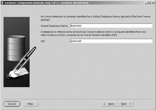
There are only a few screens requiring input when a preconfigured database is used. The next is that for naming the database, as shown in Figure 2.5, where we have called the database EASYDW.
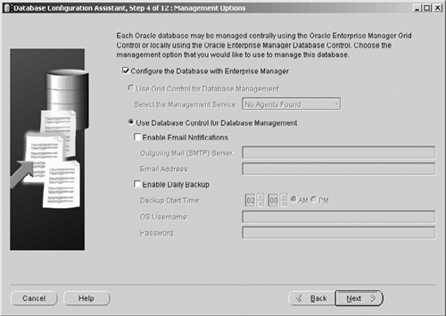
Oracle Database 10g introduces the whole concept of Database Grids and the centralized management of many databases. For the purpose of our database we are going to manage our warehouse database with the local database version of Enterprise Manager rather than the Grid Control version. (See Figure 2.6)
The next step, shown in Figure 2.7, is to enable the passwords for the critical Oracle accounts to be set. For simplicity in our warehouse, we will use the same password for all accounts: In a true production system you may well want to have different passwords to heighten the security on your system.

Now comes one of the new steps in Oracle Database 10g which gives us our first flavor of some of the new Oracle Database 10g features. In the next step, shown in Figure 2.8, we must decide how we want our database files stored on our disks.
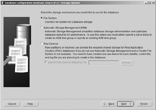
There are three options:
Using the File System (i.e., stored as normal files)
Using Automatic Storage Management (ASM). For this option you must identify a set of disks to Oracle, which it can use solely for its database files.
Using Raw Devices. A disk option, where disks are used without file systems, which is an option to enable Real Application Clusters (RAC) to be used.
For now, we will use option 1 to store the database files in the file system, but in Chapter 3 we will look more closely at both RAC and the new ASM option.
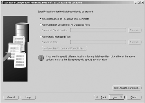
Because we have chosen option 1 to use the file system, the next screen, shown in Figure 2.9, provides us with some control over how and where the files are placed in the file system. If we had chosen either option 2 or 3, then we would get different screens at this stage.
Oracle Database 10g introduces new options for backup and recovery, including Flashbackup to disk in the Flash Recovery Area, where the disk usage is managed by Oracle. The next step, shown in Figure 2.10, enables the specification of the disk area for Flash Recovery and the amount of disk space to be allocated.

The ORACLE_BASE notation shown for specifying the Flash Recovery Area forms part of the directory structure of an Oracle installation. ORACLE_BASE denotes the directory of the root of the Oracle subdirectories, and ORACLE_HOME, which you will also see mentioned, denotes the directory that contains the software specific to this Oracle Database 10g installation—for example:
ORACLE_BASE = C:oracleproduct10.1.0
ORACLE_HOME = C:oracleproduct10.1.0Db_1
You may also see ORACLE_HOME written as ORACLE_BASE Db_1.
In Figure 2.10, the Flash Recovery Area is being placed in a subdirectory off ORACLE_BASE. The Flash Recovery area on disk should normally be distinct and separate from that used for the database files.
Along with these features there are some sample schemas that can be installed, where examples are provided to help illustrate the functionality available in these features. This is shown in the screen in Figure 2.11, where there is also the option for some custom scripts to be executed.

The next step is to define some of the parameters used to configure the database. Oracle Database 10g has a number of components that can be configured. In Figure 2.12, we see step 5 of 7 from the Database Configuration Assistant, where we can define the parameters for the respective areas by clicking on the appropriate tabs, which include:
Memory
Sizing, which enables the size of the database blocks to be specified and the number of processes that can connect to the database
Character set of the database
Connection mode for how client connections connect to the database
Database initialization parameters

For the sizing, the option to specify the database block size defines the lowest level of granularity and control you have concerning the allocation of space in the warehouse. It is recommended that your data warehouse be created with a large block size, such as 16,384 bytes, which means that you can store more records of the same type together in a single block, thus helping to reduce our I/O demands.
The default parameters may be suitable for your environment. However, if you need to amend them, perhaps if the memory available to you is limited—for example, you may have two databases running on one server—then click on the Custom option and amend the memory being allocated. You can see the effect of your changes instantly by monitoring the Total Memory for Oracle value.
Hint
If a parameter is set too low, you will be advised and given an opportunity to increase its value.
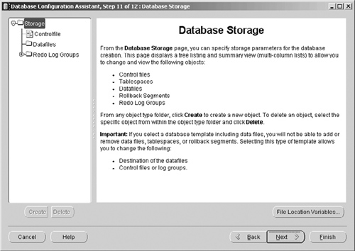
Clicking Next displays Figure 2.13 where one of the buttons is the File Location Variables. When the database is created, the location of all the files that comprise the database—that is, the data files, control files, initialization, redo log, and archiving files are located according to the values of these parameters that you can configure for each database, as illustrated in Figure 2.13. Also at this time you can define your own variables and use these in the definition of your database.
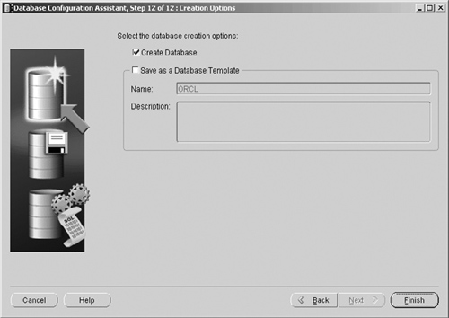
Finally, we get to the point where we can hit the Finish key for the database to be created. This screen also enables a template of your database creation script to be generated for future reference.
When using one of the preconfigured databases, you cannot control the size of the database, only the location of the files, which is the screen shown in Figure 2.13. By default all of the files are placed in one director; therefore, if you want them on different disks, now is the time to specify the new location.
All the information needed to build the database has now been defined, and you can now create the database (see Figure 2.14) or save this definition as a template for use another time. You can monitor its progress as it is being built. Once the build has finished, it is now available for use.
Now that we have a database, all objects defined in an Oracle database must reside inside a schema, a logical structure that describes a collection of objects. Therefore, before any tables are created, you should decide how many schemas you require. A data warehouse can contain anything from only a few tables for a simple warehouse up to many tens of tables for a complex, enterprise-wide warehouse, but it is still probably a good idea to keep them all in one schema to assist with their management.
However, you may prefer to create multiple schemas by subject area, but this approach will also increase the effort required to manage the database to make the information in the tables available, because there will be extra tasks to perform such as granting access to tables and defining synonyms.
Hint
It is very important to make this decision at the outset of the design, because the schema name plays an integral part in the naming convention used to retrieve information from the database.
A schema object is created every time a database user is defined. A user is created via the SQL CREATE USER statement or from within Oracle Enterprise Manager. To do this we must first logon to Enterprise Manager using a DBA account. We will discuss this more fully in Chapter 11, but for now, direct your browser to the following URL, which will display the Enterprise Manager login screen.
http://<hostname>:<port>/em
For example, if you have installed Oracle on a standalone server and opted for local management via Enterprise Manager as opposed to Grid Management, then Enterprise Manager is accessed via the previous URL. The normal port number on Windows is 5500, but this can vary depending on other installations that may have reserved that port. So if the database is on server “easydwsvr,” then the URL will be:
http://easydwsvr:5500/em
Once you have logged in, you see the initial database summary home page shown in Figure 2.15.
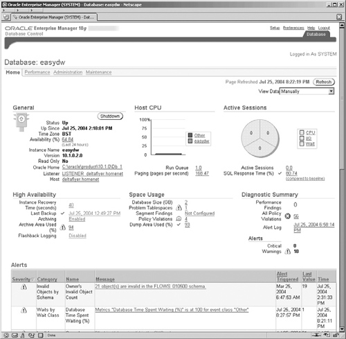
Most of the browser screens for Enterprise Manager contain in excess of one typical screen’s worth of information and are normally accessed by use of the scroll bar on the right-hand side. Our screen shots will generally only show the top section of the browser screen. At the top left there are a number of links for tabs for various other screens. Select Administration and you will see the screen shown in Figure 2.16. This may seem a little busy, but you will notice that there is a logical grouping into areas for different operations and each link takes you to a specific screen for the administration of that operation.
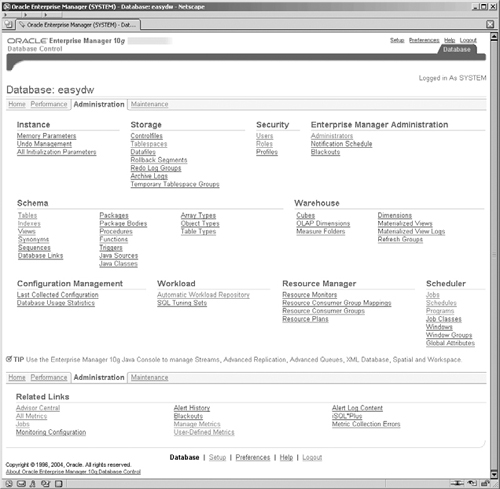
In the middle of the top row of groups entitled Security, select the Users link to get to the screen shown in Figure 2.17. This screen shows you all of the existing users in your database and enables you to select and modify these user accounts. We want to create a new user account. Click on the Create button on the right-hand side above the list of existing users to display the screen shown in Figure 2.18.

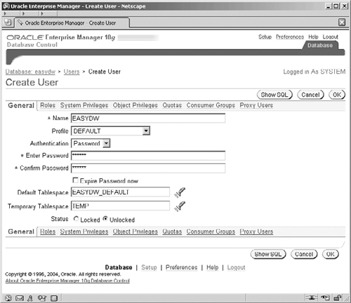
In our Easy Shopping example, we have decided to create a user called EASYDW. Here we can specify how the user will be authenticated, and we have selected the default mode of by password. This means a password must be specified and is used for all subsequent database access. Oracle permits other options for authentication, which include external for authentication via the operating system or network service, or global if performed by an LDAP-type directory service. If, in the future, this password needs to be changed, then it can be done from within Oracle Enterprise Manager, using the screen shown in Figure 2.18 or via SQL.
We must also select a default area where objects created by this user, such as tables and indexes, will reside. In a well-designed database, this is not an issue, because every object will explicitly state the tablespace in which it must be stored. There are a number of other options that can be specified for a user, such as privileges. It is important to set these; otherwise, you will not be able to retrieve data. As we progress through this book, you will be advised about which privileges are required when a topic is discussed—for example, Summary Management.
When the user is created, a schema is automatically created with that user name. However, you will not be able to see the schema name until the first object, such as a table, is defined for that user.
The schema name is very important, because it is used to fully qualify an object in the database. For example, we could have a table called TIME in the EASYDW schema and also in our ORDERS schema. To advise the optimizer which table you wish to retrieve data from, you specify the table name as :
schema name.table name
Therefore, to retrieve all the records in our time dimension, the fully qualified table name would be:
SELECT * FROM easydw.time;
You can create as many users of the database as you require, but it is recommended that only one of them be used for the purpose of creating objects, such as tables and indexes. Therefore, when the DBA connects as user EASYDW, all the tables and indexes created will reside here. In section 2.3.11, we will discuss enabling privileges for a user.
Once the database has been created, you can now add your own data files and tablespaces. By default, you will find a number of data files; on a Windows (e.g., NT, 2000, or XP) system, they will be located in:
<ORACLE_HOME>Oradata<database name>
and will comprise three control files, two system spaces (system and sysaux), the undo, the example, and the user areas. In Oracle Database 10g, the SYSAUX tablespace is new and is an additional collective tablespace used by some Oracle components and products that require their own schema and therefore have their own database objects. It should ease administration by having the objects reside in the same tablespace. This is SYSAUX.
The tablespace is the logical name that is used within the database schema to specify where objects must reside; a tablespace has one or more data files associated with it, where objects are actually stored. Part of the tablespace definition is physical location and size of these data files; therefore, an object placed in a tablespace is actually stored in these files.
In our Easy Shopping Inc. example, we have decided to implement the following tablespaces:
Dimensions—for all dimension data
Default area, which users are assigned by default
Summary—for the materialized views we will create
One tablespace for each month of the year, named Purchases_<month>_<year>, for example, PURCHASES_JAN_2003
Indx tablespace—for indexes
Temp area—for temporary space
In this example, we will create only one data file per tablespace, but, of course, you can create more if required. Also, the files shown here will be very small, and in the real world, they could be extremely large.
These tablespaces and their associated data files can be created either directly from SQL or by using Enterprise Manager, illustrated as in Figure 2.19.
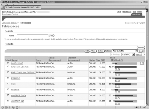
One of the advantages of using Enterprise Manager to manage your database is that it means that you no longer have to keep querying the metadata in the data dictionary tables and views to find out the state and information on objects in your database. This information is already available via the graphical interface in Enterprise Manager.
In Figure 2.16, we saw the EASYDW database Administration screen. We now select Tablespaces from the Storage group and we can see a list of tablespaces, their size, current state, and space used. This is shown in Figure 2.19.
Creating a tablespace using Oracle Enterprise Manager is very easy. From the Tablespaces screen click the Create button to navigate to the Create Tablespace screen shown in Figure 2.20 to create our Dimension tablespace where the parameters for our tablespace can be specified.

The first step is to enter the name of the tablespace. It is wise to choose sensible names, because you will be using these constantly throughout the schema, and it helps if they mean something to you. For example, the tablespace called DIMENSIONS will be used to hold the dimension tables, whereas the purchases made in January are held in a tablespace called PURCHASES_JAN2003. Another favorite approach is to suffix all data tablespaces with a D and indexes with an X to identify the type of data that is held in that tablespace.
Provide the new tablespace name in the top Name field and accept the defaults in the other fields. The Locally Managed tablespaces and Dictionary Managed options control how the space within the tablespace is managed, either by using the database data dictionary or by storing the information locally within the tablespace itself. It is becoming standard practice to use locally managed tablespaces, because this removes the overhead of accessing the data dictionary, which contains the metadata about all of the objects in the database. Locally managed tablespaces are more efficient than dictionary managed ones and hence should be preferred.
We also want our tablespace to be Permanent for our data (rather than for temporary sort usage or for transaction undo information) and we also want to be able to update, insert, and delete the objects in our tablespace. Select Add in the Datafiles section to display the screen in Figure 2.21, which enables us to add the actual files to the tablespace where our data will reside.
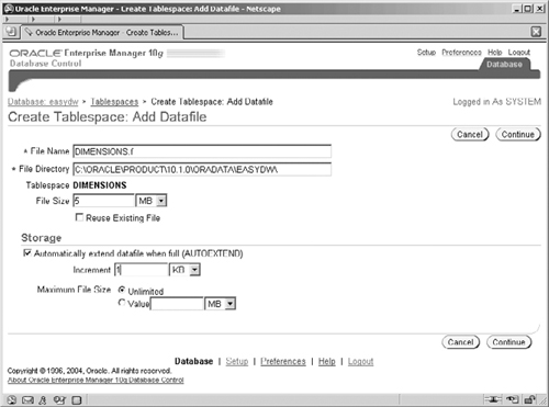
Complete the datafile information, which just consists of specifying the “dimensions.f” file name and a size of 5M. At this point you can also set the file to automatic allocation. Some designers do not like files that automatically extend; however, many do, because it means that a task will not fail simply because there is no space left in the database. Instead, the datafile will automatically extend itself, and you have control over how large those extents are. Of course, when the disk is full, autoextend will fail regardless. Selecting the Continue button returns you to the screen shown in Figure 2.22.

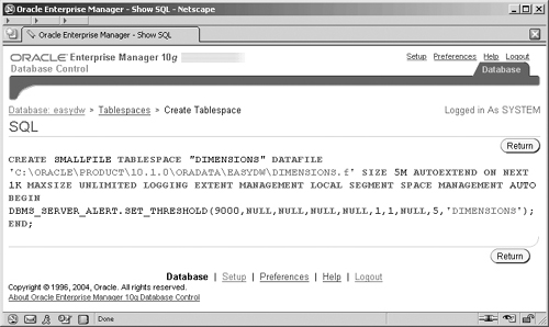
If you prefer to create your tablespace directly from SQL, then you can use either the SQL*Plus tool or the new browser-based i*SQLPlus tool (accessed from the browser at url http://<server>:5560/isqlplus). If you are uncertain of the SQL required to perform a task, you can click on the Show SQL button in most of the Enterprise Manager screens and a new screen containing the SQL will be displayed, as shown in Figure 2.23, for our tablespace creation example.
Now that we have a database, and the tablespaces and users are defined, we are ready to create the fact and dimension tables. The fact and dimension tables are created as if they were any ordinary tables inside the database. Therefore, all the options that one would specify on a table, such as the initial and subsequent extent size, may be specified. Although we call them “fact” and “dimension” tables, they are no different from any other table in the database.
When defining the fact table, carefully select the column data types, because selecting one that occupies too much space—when your fact table contains hundreds of millions of rows—will result in a considerable waste of disk space and also potentially result in performance problems if many disk blocks must be accessed to satisfy a command.
Tables are created using the SQL CREATE TABLE command, but we will now see how to create tables quickly using Enterprise Manager. For the moment, a dimension table is defined as if it were any other table in the database. In Chapter 8, we will see how to define an actual dimension object, which will be based on the table that we create here. In fact, the dimension table created at this stage is a prerequisite for creating a dimension object.
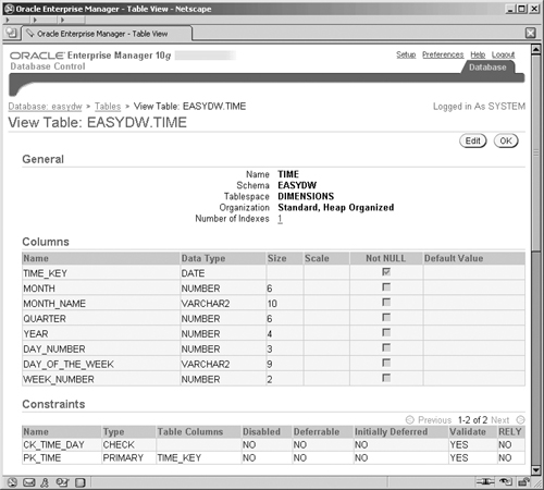
When Oracle Enterprise Manager Console is started, go to the Administration screen and in the Schema group select the Tables option, then the Tables screen shown in Figure 2.24 is displayed.

Select the Create button on the right-hand side, and on the new Table Organization screen (not shown) accept the default Standard, Heap Organized option and select Continue to get to the actual Create Table screen shown in Figure 2.25. We will discuss an alternative organization, index-organized tables, in Chapter 4.
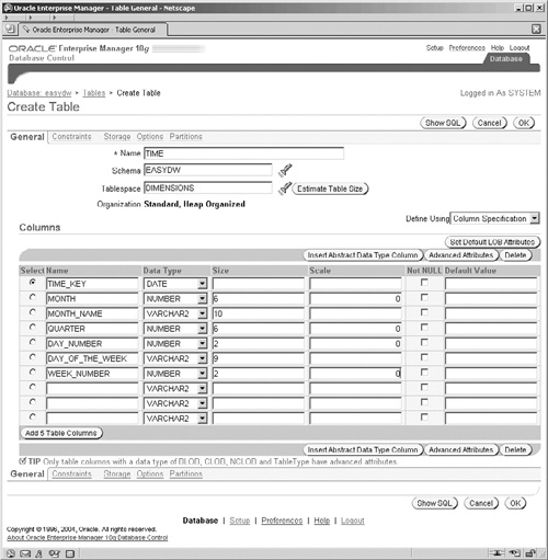
In the screen in Figure 2.25, you specify the name of the table, TIME, the schema in which it will reside, and the tablespace for this table. This is a really nice screen for quickly creating the table. All you have to do is enter the column name in the Column list in the lower half of the screen, and select the data type and its size. If you run out of lines for defining your columns, select the Add 5 Table Columns button and five new column lines will be created for you.
Define each column using this approach, and don’t click on the OK button until you have defined all of the columns in the table.
Once all of the columns in the table have been defined, clicking on the Constraints tab in the top left of this screen will allow you to create the constraints for this table.
The job of the constraint is to ensure that all data conforms to its rules, such as a value corresponds to a specified range of values via a CHECK constraint. If a primary key is defined, then this guarantees that the value in the primary-key columns in the table is unique. A foreign key will ensure that all values correspond to one of the primary keys in another table.
Mention constraints to designers, and they will probably tell you that they do not want them in the database, because they are an overhead, especially when new data is being loaded. It is highly recommended that you implement at least primary- and foreign-key constraints, especially if you wish to use the Summary Management feature that is described in Chapter 7. One of the interesting aspects of Summary Management is the ability for the database to transparently rewrite a query to use a materialized view. If you have defined constraints in your database, then it will be possible to do some complex forms of query rewrite.
In a data warehouse, there is often concern that, because the data can come from many sources, it may not be as “clean” as normal data, and, therefore, constraints may fail. Although this is a valid concern, clean data should always be stored in the warehouse to ensure that accurate results are returned.
Another argument put forward for not implementing constraints is that validating every record when it is first inserted into the database imposes a considerable burden on the load operation. Therefore, it takes considerably longer than via a standard load, and if the loading window is very small, then one way to reduce the time is not to have constraints.
In Oracle, many of these concerns can be overcome thanks to some options on the constraint:
ENABLE NOVALIDATE
DISABLE NOVALIDATE
If you are still concerned about the overhead of having constraints and worried that your data isn’t clean enough to get past the constraint checks, you can use the ENABLE NOVALIDATE clause, which turns on a constraint and applies it against all new inserts and updates, but it doesn’t check existing records. It is enabled immediately, but you should be aware that incorrect results could be returned if existing rows in the table have violated the constraint.
By using the ENABLE NOVALIDATE clause, as illustrated in the following code segment, we can turn on the constraint SYS_C001136 without having to validate all of the data.
ALTER TABLE todays_special_offers
  ENABLE NOVALIDATE CONSTRAINT SYS_C001136;
Therefore, if we know or want to assume that the data is clean, we can just turn on the constraint immediately without incurring any overhead. Using this approach, the database doesn’t spend time validating the constraint against all the rows in the table, but it does mean that the designer had better be certain that the data is clean.
Hint
Use sensible constraint names, such as customer_pkey, which will mean so much more than SYS_C001136.
Likewise, before data is loaded, the constraints can be quickly disabled using the DISABLE clause, as shown in the following code segment:
ALTER TABLE todays_special_offers
     DISABLE CONSTRAINT SYS_C001136;
The ETL stage, when we load our warehouse, can also be used to programmatically validate the constraint candidates—for example, using PL/SQL, resulting in the constraints being implemented as “disabled novalidate.” This means that the data is already checked and the constraint is not enabled for new inserts or updates and does not validate the data already in the table.
Oracle Database 10g Enterprise Manager now supports the ability to specify the ENABLE/DISABLE and VALIDATE/NOVALIDATE clauses.
There is an additional clause called RELY, which is used by the summary management feature. This clause tells the optimizer that you can rely on the accuracy of the constraint. An example of using the RELY clause is shown in the following code on a constraint in the TODAYS_SPECIAL_OFFER table. Chapter 9 will discuss how RELY constraints are used by summary management.
ALTER TABLE purchases MODIFY CONSTRAINT special_offer RELY;
You can check the constraints that have been defined in your database from the Tables screen. Select the table from the Tables screen list and then the Edit button to navigate to the Edit Table screen; then click on the Constraint tab to get the screen shown in Figure 2.26.

In Figure 2.27, we see how to create a primary key. Not every table in our data warehouse, such as the fact table, will have a primary key, but some of the columns may require that they are not null.
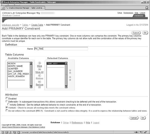
For the Constraints screen while editing the TIME table, ensure that “PRIMARY” is displayed in the pick list box on the right-hand side and select the Add button.
Enter the name to use as the constraint name. Again, a good naming convention for constraint names is invaluable. We suggest using the following suffixes or prefixes to indicate the constraint type:
PK for primary key
UK for a unique constraint
FK for a foreign-key constraint
CK for a check constraint
Enter PK_TIME in the Name field, then select the column that forms the primary key from the Available Columns list, and select Move to move it into the Selected Columns box. If more than one column forms the primary key on your tables, then this operation is repeated for each of the required columns.
Select the attributes that you want the new primary-key constraint to have (enable/disable, validate/novalidate, etc.) and select Add to create the constraint on the database.
From the same Constraints tab on the Edit Table screen, check, unique, or foreign-key constraints can be similarly defined. A check constraint enables you to specify a condition that must be true for the columns for every row in the table. In our example in Figure 2.28, we have specified that the column DAY_NUMBER may take only the values between 1 and 366. Therefore, before a value is stored in this database, a check is automatically made by the database server that the column takes one of these values.

An alternative to using the GUI to obtain information from Oracle Database 10g is to query the many system data dictionary tables and views that are available; these provide a wealth of information about the state of your database and objects. In the following code, we can see the information held about constraints in the view USER_CONSTRAINTS.
SQL> DESCRIBE user_constraints
 Name                                   Null?    Type
 ----------------------------------- -------- ------------
 OWNER                               NOT NULL VARCHAR2(30)
 CONSTRAINT_NAME                     NOT NULL VARCHAR2(30)
 CONSTRAINT_TYPE                              VARCHAR2(1)
 TABLE_NAME                          NOT NULL VARCHAR2(30)
 SEARCH_CONDITION                             LONG
 R_OWNER                                      VARCHAR2(30)
 R_CONSTRAINT_NAME                            VARCHAR2(30)
 DELETE_RULE                                  VARCHAR2(9)
 STATUS                                       VARCHAR2(8)
 DEFERRABLE                                   VARCHAR2(14)
 DEFERRED                                     VARCHAR2(9)
 VALIDATED                                    VARCHAR2(13)
 GENERATED                                    VARCHAR2(14)
 BAD                                          VARCHAR2(3)
 RELY                                         VARCHAR2(4)
 LAST_CHANGE                                  DATE
 INDEX_OWNER                                  VARCHAR2(30)
 INDEX_NAME                                   VARCHAR2(30)
 INVALID                                      VARCHAR2(7)
 VIEW_RELATED                                 VARCHAR2(14)
Every constraint that you define for this schema will be recorded in this data dictionary view. All of these views provided by Oracle will be prefixed either ALL_, USER_, or DBA_. Those prefixed DBA can only be accessed by user accounts with the DBA role assigned to them, those prefixed USER show information about your own accounts objects, and those prefixed ALL show information about other users’ objects to which you have been granted privileges.
For example, to see on which constraints you have used the RELY clause, use the following query:
SQL> SELECT constraint_name, table_name, rely FROM all_constraints
     WHERE OWNER = 'EASYDW';

CONSTRAINT_NAME                TABLE_NAME                RELY
---------------------------- ------------------------- ----
COST_PRICE_NOT_NULL          PRODUCT
FK_CUSTOMER_ID               PURCHASES
FK_PRODUCT_ID                PURCHASES
FK_TIME                      PURCHASES
NOT_NULL_CUSTOMER_ID         PURCHASES
NOT_NULL_PRODUCT_ID          PURCHASES
NOT_NULL_TIME                PURCHASES
PK_CUSTOMER                  CUSTOMER
PK_PRODUCT                   PRODUCT
PK_SPECIALS                  TODAYS_SPECIAL_OFFERS
PK_TIME                      TIME
PUBLIC_HOLIDAY               TIME
SELL_PRICE_NOT_NULL          PRODUCT
SHIPPING_CHARGE_NOT_NULL     PRODUCT
SPECIAL_OFFER                PURCHASES                 RELY
Here we can see that the constraint SPECIAL_OFFER has the RELY clause enabled, whereas constraint SHIPPING_CHARGE_NOT_NULL does not. In Figure 2.29, we can see the constraints that have been defined on the table TIME.
The main Constraint tab for a table will also show you the full status of the constraints on your table. This information can also be determined by querying one of the constraint system tables, such as ALL_CONSTRAINTS. For example, to see which constraints have been enabled using the NOVALIDATE clause, use the following query:
SQL> SELECT constraint_name, validated FROM all_constraints
  WHERE OWNER = 'EASYDW';

CONSTRAINT_NAME                VALIDATED
------------------------------ -------------
PK_CUSTOMER                    VALIDATED
COST_PRICE_NOT_NULL            VALIDATED
SELL_PRICE_NOT_NULL            VALIDATED
SHIPPING_CHARGE_NOT_NULL       VALIDATED
The definition of the table is almost complete. We have defined the columns and the constraints that are required, and we could press the Finish button, but there are two more categories of information that the table wizard requests, storage and partitioning, which will be described later.
If you are happy with the table definition that you have entered (and you can check the SQL that will be applied by using the Show SQL button: see Figure 2.30), then press the Apply button; otherwise, select the correct tab and amend the entry accordingly.

Hint
In order to create an object (e.g., table or index) in a tablespace, the user must have a quota in that tablespace. Go to the Users screen and edit the EASYDW user and select the Quotas tab: from here you can assign the space quota EASYDW has on a tablespace.
When you click on the OK button on the Create Table screen, the table is created, and you are now ready to create the next table. Hopefully, you will agree that this is a very easy way to create a table, and, since a data warehouse probably only has a few tables, you may prefer to use this friendly approach as opposed to writing SQL commands, where you will probably make many syntax errors that you will have to correct.
A data warehouse is likely to contain a number of indexes, and, just like any other database, the designer must choose the indexes that are most suitable. Oracle offers several different types of indexes, but the ones that will be of interest to the data warehouse designer are:
B*tree index
Bitmapped index
Bitmapped join index
Indexes should be selected carefully, and the various options and reasoning behind certain choices will be described in detail in Chapter 4. Please consult this chapter, because there you will learn whether to select a global or local index and how to partition it, if required.
To set the scene for this section, a bitmapped index is ideally suited to the data warehouse environment when you want to index a column that takes only a few values. For example, suppose we wanted to index the column PUBLIC_HOLIDAY, which has only two values: Y or N. A bitmapped index will store this information in an extremely compact manner, and this also has additional benefits for the way that the Oracle optimizer accesses the data for typical warehouse queries.
Although indexes easily can be dropped and created, due to the time required to create them, especially on a fact table with millions of rows, careful planning at the outset of the project will ensure that you won’t have to spend a lot of time creating the index. An index can be created by using either the SQL CREATE INDEX command or Oracle Enterprise Manager.
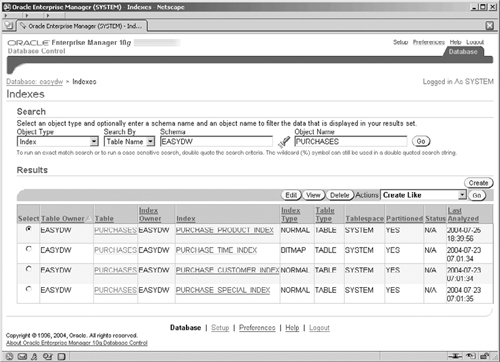
Figure 2.31 shows the Indexes screen, which can be accessed from the Schema section on the main EM Administration screen. Completing the Schema and Object Name fields and selecting Go displays the indexes for that object.
Partitioning data is a design technique that is very important in the warehouse, because it provides a means of managing large amounts of data and controlling its placement on the disks. Rather than place all of the data from a table in one tablespace, partitioning enables us to place the data in many tablespaces. Partitioning enables easier management of our tables and also enables the optimizer to use better techniques to access the data by only accessing the relevant partitions; this results in better performance. To determine how the data in a table is split into the different partitions (and therefore in which tablespace the data is stored), a partition key is selected, such as time_key, as illustrated in Figure 2.32.

In this example, we are partitioning by month, so January’s data goes in one partition, February’s in another, and so forth. You must select the partition key carefully, although a common one is by time. Therefore, you could partition data by month, and then each month would reside in its own tablespace. This helps result in a more manageable partition, and it also has the advantage that if you ever had to archive the data, it would be as simple as dropping a partition. Of course, don’t forget to back up the partition before you drop it! Dropping a partition is a very quick process and doesn’t invalidate any of the data that is already in the fact table.
Oracle Database 10g provides several different types of partitioning techniques, and, after reading the partitioning section in Chapter 4, you can select the one that is most appropriate for your data warehouse. We will defer walking through the table partition screens of Enterprise Manager until Chapter 4, where the subject is dealt with in more detail.
We have already seen that a data warehouse or data mart can hold a huge number of records in the fact table. Even if we had the fastest machine in the world and could cache some of the data warehouse in memory, the time required to respond to queries could be days—and it would certainly be minutes or hours.
To overcome this problem, warehouse designers use the technique of creating summaries, a summary being a preaggregated table of results, which Oracle calls a materialized view (MV). For example, suppose you always query on the number of purchases of today’s special offer by day. Rather than compute those results every time, a materialized view is created that contains the required information. Then, whenever you make this query, instead of querying the fact table, you query the materialized view.
Although it partially defeats the object of a warehouse when you make unknown queries to the database, it is fair to say that quite a few queries upon the warehouse are well known. If we can improve the response time on those queries, then our users will be very grateful.
Oracle Database 10g includes a specific summary management component, which will enable you to create materialized views rather than ordinary tables, and then the optimizer will transparently rewrite your query to use the materialized view. This feature is described in detail in Chapter 9. At this stage of the design, if you can identify any queries that would lend themselves to being created as materialized views, they should be recorded now for subsequent creation. Some examples of the materialized views that we might create for our Easy Shopping Inc. examples are:
Sum of sales by product by day
Count of products sold by day
Sum of sales by week
Profit by product by day
If you don’t know what materialized views you will need, then you can use the SQL Access Advisor, which has a number of methods to assess and create potential MVs: This is explained further in Chapter 10. Because some materialized views can be large, the number that you expect to create will impact how many tablespaces and data files should be defined for this data warehouse. For example, large materialized views may be partitioned in the same manner as we have partitioned tables, and the ease of management of these partitions is facilitated by using more than one tablespace in the same way as it does for partitioned tables.
Hint
It’s not necessary to create a materialized view for every possible combination; this will all be explained in Chapters 7 to 10.
One should not forget that some data in the warehouse could be very sensitive, and, therefore, for a variety of reasons, you may not want all of your staff to have access to it. Oracle Database 10g provides various types of security, which prevents users from changing the objects inside the database and accessing data.
Privileges can be granted on objects in our schema to permit the type of access that other users have on these objects. For example, reading the data in a table, updating the data, or deleting the data is provided by three different privileges granted to a user on the table. Different object privileges can be placed on a variety of objects, including the following:
Tables
Views
Sequences
Synonyms
PL/SQL modules
Types
Queues
You will most likely place security on tables and views, by stating whether a user can select, insert, and update the data, along with a number of other options. If you decide to create a number of users, then always ensure that sufficient privileges have been allocated so that everyone can read the data. This can be achieved by using either the SQL command, GRANT SELECT ON for a table, or the GRANT SELECT ANY TABLE, or these privileges can be allocated directly to the user name using Oracle Enterprise Manager, within the Security section.
In Figure 2.33, we are giving a user of our warehouse, user EASY-DWUSER, the rights to ALTER, INSERT, SELECT, and UPDATE the TIME table in the EASYDW schema. This screen is accessed from the Tables screen by selecting the EASYDW table TIME, selecting Grant Privileges in the pick list box on the right, and selecting the Go button. Simply repeat this process for each user and the tables that he or she is allowed to access.

Alternatively, you could create a role. Then you assign all of the privileges to the role, and the role is assigned to the user. This is the preferred approach, because it provides easier management and control of the privileges—especially if you create many users, because then you can create roles for the different job levels, and each user is granted one of those roles instead of assigning the privileges individually. Using the role approach, you reduce the likelihood of users accidentally being given access to data that they shouldn’t have. It is also quicker if many users have to be defined. You can either use existing roles or create your own role using the SQL CREATE ROLE statement.
Most of the time will be spent granting object privileges to users and maybe creating roles. However, some users will require system privileges. A system privilege is one that gives you the right to perform high-level tasks, such as creating or dropping a table. Since you will not want to grant this right to many users, you shouldn’t have to spend too much time giving system privileges.
The method used to define a system privilege is to select the target user from the list on the Users screen, select the Edit button, and then select the System Privileges tab on the Edit User screen. In a data warehouse, there are some specific system privileges that you may want to grant to specific users, such as CREATE DIMENSION and CREATE MATERIALIZED VIEW. In this instance, you would only be granting this privilege to users who would create dimensions and materialized views.
Our database is almost complete, but there is one other important feature available in Oracle Database 10g that should be mentioned, and that is the parallel clause. A number of the statements shown here can be executed in parallel, and the use of this technique is very important in a data warehouse, because it can significantly improve statement execution time. Parallel operations are available on table scans, sorts, joins, aggregates, and some table and index operations.
If you are using a symmetric multiprocessor system, then serious consideration should be given to using the PARALLEL clause. When specified, a statement, if eligible for parallel processing, will be decomposed into a number of parallel threads, and Oracle Database 10g will perform the job using parallel tasks and coordinate their running and the results. Therefore, all the user has to do is include the clause, and Oracle Database 10g does the rest.
The PARALLEL clause will expect you to specify the number of parallel processes to use. Choose this value carefully. Some testing may be required to determine the optimum value. For example, the following clause could be added to the CREATE TABLE statement for our purchases fact table:
PARALLEL (DEGREE 2)
This would mean that any operations on this table should be done using two server processes if they can be executed in parallel.
Data may also be loaded in parallel. The SQL*Loader facility, which we will discuss later, allows you to request parallel operations. Obviously, this can significantly improve the time required to store data; however, you should be aware of the possible fragmentation of your data that could occur. Therefore, it is suggested that, when data is being loaded in parallel, you specify the number of parallel operations to be equivalent to the number of datafiles available for that tablespace. Therefore, referring to our Easy Shopping Inc. example, if we decided to specify a value of:
PARALLEL (DEGREE 3)
on our purchases table, there should be three datafiles defined for every tablespace.
More importantly, Oracle Database 10g also has the facility to automatically control the degree of parallelism based on other criteria, such as number of users and other queries currently executing in the database. In this case, a degree does not have to be specified and only the keyword PARALLEL is used to activate parallelism for the particular object.
None of us would write an application and send it live without testing it first. But it is amazing how many database designs are constructed and then unleashed on unsuspecting users. Your data warehouse is no different, especially since the business is relying on it for important information. Therefore, it is very important that all aspects of the design and processes are thoroughly tested prior to production release.
It is suggested that you initially load a small percentage of the data into the warehouse, and then test the following areas:
If you are building a terabyte-size warehouse, then it is recommended that you repeat this process again with even more data in the warehouse, just in case there are any unexpected problems dealing with this volume of data.
Problems identified during testing are much easier to fix than trying to resolve them once the warehouse has gone live. A phased implementation to the user base is another way to test the warehouse if you don’t want to wait until all of the testing is complete.
One very important point to remember is that, due to the size of the data warehouse, it will not only take much longer to load the data, but it is also unlikely that queries will complete quickly. Therefore, the entire testing process will take much longer than, say, a traditional OLTP database.
We have seen in this chapter how to create our database using the GUI tools, but many readers may prefer to create the database directly from SQL. The SQL to achieve this is shown in Appendix A.
Our database is now complete. We have a basic framework, and now we will learn in the next chapter how to enhance our basic database design to include and use the sophisticated features that are available in Oracle Database 10g.