
Populating a data warehouse involves all of the tasks related to getting the data from the source operational systems, cleansing and transforming the data to the right format and level of detail, loading it into the target data warehouse, and preparing it for analysis purposes.
Figure 5.1 shows the steps making up the extraction, transformation, and load (ETL) process. Data is extracted from the source operational systems and transported to the staging area. The staging area is a temporary holding place used to prepare the data. The staging area may be a set of flat files, temporary staging tables in the Oracle warehouse, or both. The data is integrated with other data, cleansed, and transformed into a common representation. It is then loaded into the target data warehouse tables. Sometimes this process is also referred to as ETT—extraction, transportation, and transformation.
During the initial population of the data warehouse, historical data is loaded that could have accumulated over several years of business operation. The data in the operational systems may often be in multiple formats. If, for instance, the point-of-sales operational system was replaced two years ago, the current two years of history will be in one format, while data older than two years will be in another format.
After the initial historical load, new transaction and event data needs to be loaded on a periodic basis. This is typically done on a regular time schedule, such as at the end of the day, week, or month. During the load, and while the indexes and materialized views are being refreshed, the data is generally unavailable to warehouse users for querying. The period of time allowed for inserting the new data is called the batch window. The batch window is a continuously shrinking amount of time as more businesses are on-line for longer periods of time. Currently, with the ability to refresh the warehouse in real time, or near real time, batch windows are becoming a higher priority and requirement as businesses want and need to react to changes in a more immediate fashion. Higher availability can be achieved by partitioning the fact table. While data is loaded into a new partition, or being updated in an existing partition, the rest of the partitions are still available for use.
A large portion of the work in building a data warehouse will be devoted to the ETL process. Finding the data from the operational systems, creating extraction processes to get it out, transporting, filtering, cleansing, transforming, integrating data from multiple sources, and loading it into the warehouse can take a considerable amount of time.
If you are not already familiar with the company’s data, part of the difficulty in developing the ETL process is gaining an understanding of the data. One object can have different names in different systems. Even worse, two different things could have the same name. It can be a challenge to discover all of this, particularly in a company where the systems are not well documented. Each column in the target data warehouse must be mapped to the corresponding column in the source system. Some of the data will be mapped directly; other data will need to be derived and transformed into a different format.
Once the data is loaded into the warehouse, further processing to integrate it with existing data, update indexes, gather statistics, and refresh materialized views needs to take place prior to it being “published” as ready for users to access. Once the data is published, it should not be updated again until the next batch window, to ensure users do not receive different answers to the same query asked at a different time.
Once you have identified the data you need in the warehouse for analysis purposes, you need to locate the operational systems within the company that contain that data. The data needed for the warehouse is extracted from the source operational systems and written to the staging area, where it will later be transformed. To minimize the performance impact on the source database, data is generally extracted without applying any transformations to it.
Often the owners of the operational systems will not allow the warehouse developers direct access to those systems but will provide periodic extracts. These extracts are generally in the form of flat, sequential operating system files, which will make up the staging area.
In order to extract the fields and records needed for the warehouse, specialized application programs may need to be developed. If the data is stored in a legacy system, then these programs may require special logic—for example, if written in COBOL—in order to handle things such as repeating fields in the “COBOL occurs” clause. The data warehouse designers need to work closely with the application developers for the OLTP systems that are building the extract scripts to provide the necessary columns and formats of the data.
As part of designing the ETL process, you need to determine how frequently data should be extracted from the operational systems. It may be at the end of some time period or business event, such as at the end of the day or week or upon closing of the fiscal quarter. It should be clearly defined what is meant by the “end of the day” or the “last day of the week,” particularly if you have a system used across different time zones. The extraction may be done at different times for different systems and staged to be loaded into the warehouse during an upcoming batch window. Another aspect of the warehouse design process involves deciding which level of aggregation is needed to answer the business queries. This also has an impact on which and how much data is extracted and transported across the network.
Some operational systems may be in relational databases, such as Oracle 8i, 9i, or 10g; Oracle Rdb; DB2/MVS; Microsoft SQL Server; Sybase; or Informix. Others may be in a legacy database format, such as IMS or Oracle DBMS. Others may be in VSAM, RMS indexed files, or some other structured file system.
If extracting and transporting the data from the source systems must be done by writing the data to flat files, then there is also the issue of defining:
The file naming specification.
Which files constitute the batch—for example, if more than one source table is being read from each source system, then data in each table will probably be written to its own flat file. All of the data extracted at the same time from the source system should normally be batched together and transferred and loaded into the data warehouse as a logical unit of work.
The method for transporting the files between the source system and the warehouse—for example, is the data pushed from the source system or pulled by the warehouse system? If FTP is being used, then typically it may require a new operating system account on the warehouse server if the source system is pushing the data, but this new account will normally only be able to write to a very restricted directory area that the warehouse load processes can then read from.
Let’s consider the file naming convention, and, in particular, the situation if multiple different source systems provide their data using flat files. With this situation, it is quite typical for the file naming convention to incorporate the following:
The source system name
The date of extraction
A file batch number—particularly if there can be more than one data extraction in a business day
The source table name
A single character indicator to show whether this is an original extraction or a repeat—for example, if some corruption occurred and the data had to be reextracted and resent
Alternatively, if you are able to access the source systems directly without recourse to using flat files, you can retrieve the data by using a variety of techniques, depending on the type of system it is. For small quantities of data, a gateway such as ODBC can be used. For larger amounts of data, a custom program directly connecting to the source database in the database’s native Application Programming Interface (API) can be written. Many ETL tools simplify the extraction process by providing connectivity to the source.
After the initial load of the warehouse, as the source data changes, the data in the warehouse must be updated or refreshed to reflect those changes on a regular basis. A mechanism needs to be put into place to monitor and capture changes of interest from the operational systems. Rather than rebuilding the entire warehouse periodically, it is preferable to apply only the changes. By isolating changes as part of the extraction process, less data needs to be moved across the network and loaded into the data warehouse.
Changed data includes both new data that has been added to the operational system as well as updates and deletes to existing data. For example, in the EASYDW warehouse, we are interested in all new orders as well as updates to existing product information and customers. If we are no longer selling a product, the product is deleted from the order-entry system, but we still want to retain the history in the warehouse. This is why surrogate keys are recommended for use in the data warehouse. If the product_key is reused in the production system, it does not affect the data warehouse records.
In the data warehouse, it is not uncommon to change the dimension tables, because a column such as a product description may change. Part of the warehouse design involves deciding how changes to the dimensions will be reflected. If you need to keep one version of the old product description, you could have an additional column in the table to store both the current description and the previous description. If you need to keep all the old product descriptions, you would have to create a new row for each change, assigning different key values. In general, you should try to avoid updates to the fact table.
There are various ways to identify the new or changed data. One technique to determine the changes is to include a time stamp to record when each row in the operational system was changed. The data extraction program then selects the source data based on the time stamp of the transaction and extracts all rows that have been updated since the time of the last extraction. For example, when moving orders from the order processing system into the EASYDW warehouse, this technique can be used by selecting rows based on the PURCHASE_DATE column, as illustrated later in this chapter.
However, this technique does have some potential disadvantages:
If multiple updates have occurred to a record since the date and time of the last extraction, then only the current version of the record is read and not all of the interim versions. Typically, this may not have a significant impact on the warehouse unless it is necessary for analysis purposes to track all changes.
The query to select the changed data based on the time stamp can have an impact on the source system.
If records are deleted in the source system, then this mechanism is unsuitable because you cannot select a record that is no longer present. Converting the delete into a “logical delete” by setting a flag is normally not practical and involves considerable application change. This is where the next technique using triggers can help.
If the source is a relational database, triggers can be used to identify the changed rows. Triggers are stored procedures that can be invoked before or after an event, such as when an insert, update, or delete occurs on each record. The trigger can be used to save the changed records into a separate table from where the extract process can later retrieve the changed rows. One advantage of triggers is that the same transaction is used for writing the changed record to another table as is used to alter the source record itself. If this transaction aborts and rolls back for any reason, then our change record is also rolled back. However, be very careful of triggers in high-volume applications, as they can add significant overhead to the operational system.
Sometimes it may not be possible to change the schema to add a timestamp or trigger. The system may already be heavily loaded, and you do not want to degrade the performance in any way. Or the source may be a legacy system, which does not have triggers. Therefore, you may need to use a file comparison to identify changes. This involves keeping before and after images of the extract files to find the changes. For example, you may need to compare the recent extract with the current product or customer list to identify the changes.
Changes to the metadata, or data definitions, must also be identified. Changes to the structure of the operational system, such as adding or dropping a column, impact the extraction and load programs, which may need to be modified to account for the change.
Oracle Database 10g uses a feature called Change Data Capture, often referred to as CDC, to facilitate identifying changes when the source system is also an Oracle 9i or 10g database. CDC was introduced in Oracle 9i with just the synchronous form, where generation of the change records is tied to the original transaction. In Oracle Database 10g the new asynchronous form is introduced; this disassociates the generation of the change records from the original transaction and reduces the impact on the source system for collecting the change data. In this section, we will look at both forms and work through examples of each mechanism.
With CDC, the results of all INSERT, UPDATE, and DELETE operations can be saved in tables called change tables. The data extraction programs can then select the data from the change tables. CDC uses a publish-subscribe interface to capture and distribute the change data, as illustrated in Figure 5.2. The publisher, usually a DBA, determines which user tables in the operational system are used to load the warehouse and sets up the system to capture and publish the change data. A change table is created for each source table with data that needs to be moved to the warehouse.
The extract programs then subscribe to the source tables; therefore, there can be any number of subscribers. Each subscriber is given his or her own view of the change table. This isolates the subscribers from each other while they are simultaneously accessing the same change tables. The subscribers use SQL to select the change data from their subscriber views. They see just the columns that they are interested in and only the rows that they have not yet processed. If the updates of a set of tables are dependent on each other, the change tables can be grouped into a change set. If, for example, you had an order header and an order detail table, these two tables would be grouped together in the same change set to maintain transactional consistency. In order to create a change table, you must first, therefore, create the parent change set. A change source is a logical representation of the source database that contains one or more change sets.
In Oracle 9i only synchronous data capture existed, where changes on the operational system are captured in real time as part of the source transaction. The change data is generated as DML operations are performed on the source tables. When a new row is inserted into the user table, it is also stored in the change table. When a row is updated in a user table, the updated columns are stored in the change table. The old values, new values, or both can be written to the change table. When a row is deleted from a user table, the deleted row is also stored in the change table. The change data records are only visible in the change table when the source transaction is committed.
Synchronous CDC is based on triggers, which fire for each row as the different DML statements are executed. This simplifies the data extraction process; however, it adds an overhead to the transaction performing the DML. In Asynchronous Change Data Capture, which is introduced in Oracle Database 10g, the capture of the changes is not dependent upon the DML transaction on the source system. With asynchronous CDC, the changes are extracted from the source system’s redo logs, which removes the impact on the actual database transaction. The Oracle redo logs are special files used by the database that record all of the changes to the database as they occur. There are two forms of redo logs:
On-line redo logs
Archive redo logs
The on-line redo logs are groups of redo logs that are written to in a round-robin fashion as transactions occur on the database. When a redo log fills up, the database swaps to the next one, and if archiving of the logs is turned on (which is practically a certainty on any production database), then the database writes the completed redo log file to a specified destination where it can subsequently be safely stored. This is the archived redo log. Asynchronous CDC reads redo logs to extract the change data for the tables that we are interested in and therefore it is a noninvasive technique, which does not need to alter the source schema to add triggers to tables. The action of reading the logs in this fashion is often called mining the logs. In addition, the mining of the log files for the change data is disassociated from the source transaction itself, which reduces, but doesn’t remove, the impact on the source system.
Asynchronous CDC needs an additional level of redo logging to be enabled on the source system, which adds its own level of impact on the source database, but this is much less than that of synchronous CDC.
Asynchronous CDC can be used in two ways:
HOTLOG, where the changes are extracted from the on-line redo logs on the source database and then moved (by Oracle Streams processes) into local CDC tables also in the source database. The changed data in the CDC tables will still need to be transported to our warehouse database.
AUTOLOG, where the changed data is captured from the redo logs as they are moved between databases by the Log Transport Services. The changes are then extracted from these logs and made available in change tables on this other database. If this other database is our data warehouse database, then, by using AUTOLOG, we have removed the transportation step to make our changed data available in the staging area of the warehouse.
Log Transport Services are a standard part of the operation of the database—for example, they are used by Oracle Data Guard for moving the log files to other servers in order to maintain standby databases and as such do not add any additional impact to the source database operation.
The time between the change being committed by the transaction and it being detected by CDC and moved into the change table is called the latency of change. This is smaller with the HOTLOG method than with the AUTOLOG method. This is because HOTLOG is reading the on-line redo logs and publishing to tables on the same source system, compared with AUTO LOG, where the logs must first be switched and then transported between databases—in which case the frequency of transporting the logs is the determining factor. For HOTLOG, mining the redo logs occurs on a transaction-by-transaction basis when the source transaction commits.
In the EASYDW warehouse, we are interested in all new orders from the order-entry system. The DBA creates the change tables, using the DBMS_CDC_PUBLISH.CREATE_CHANGE_TABLE procedure, and specifies a list of columns that should be included. A change table contains changes from only one source table.
In many of the examples in this chapter, we will use a schema named OLTP, which represents a part of the operational database. In the following example, the DBA uses the CREATE_CHANGE_TABLE procedure to capture the changes to the columns from the ORDERS table in the OLTP schema.
The next two sections provide an example of the two different methods for setting up synchronous and asynchronous CDC and, following that, the common mechanism for subscribing to the change data. To do this we are going to use three new schemas:
OLTP for the owner of our warehouse source tables
OLTPPUB for the publisher of the change data that has occurred on our OLTP tables
OLTPSUBSCR for the subscriber to the change data
Our source table for both methods is ORDERS, and the other two differences between the methods to note are:
For synchronous, the change set is EASYDW_SCS and the change table is ORDERS_SYNCH_CT
For asynchronous, the change set is EASYDW_ACS and the change table is ORDERS_ASYNCH_CT
In the subscriber section, we will highlight what needs to change in order to subscribe to the change data created by these two methods.
From a DBA account, create the new accounts and create a source table in the OLTP account:
CREATE USER oltp IDENTIFIED BY oltp
  DEFAULT TABLESPACE users
  TEMPORARY TABLESPACE temp
  QUOTA UNLIMITED ON users;
GRANT connect, resource TO oltp ;

CREATE USER oltpsubscr IDENTIFIED BY oltpsubscr
  DEFAULT TABLESPACE users
  TEMPORARY TABLESPACE temp
  QUOTA UNLIMITED ON users;
GRANT connect, resource TO oltpsubscr ;

CREATE USER oltppub IDENTIFIED BY oltppub
  QUOTA UNLIMITED ON SYSTEM
  QUOTA UNLIMITED ON SYSAUX;

GRANT CREATE SESSION TO oltppub;
GRANT CREATE TABLE TO oltppub;
GRANT CREATE TABLESPACE TO oltppub;
GRANT UNLIMITED TABLESPACE TO oltppub;
GRANT SELECT_CATALOG_ROLE TO oltppub;
GRANT EXECUTE_CATALOG_ROLE TO oltppub;
GRANT CREATE SEQUENCE TO oltppub;
GRANT CONNECT, RESOURCE, DBA TO oltppub;

CREATE TABLE oltp.orders
(order_id              varchar2(8)  NOT NULL,
 product_id            varchar2(8)  NOT NULL,
 customer_id           varchar2(10) NOT NULL,
 purchase_date         date         NOT NULL,
 purchase_time         number(4,0)  NOT NULL,
 purchase_price        number(6,2)  NOT NULL,
 shipping_charge       number(5,2)  NOT NULL,
 today_special_offer   varchar2(1)  NOT NULL,
 sales_person_id       varchar2(20) NOT NULL,
 payment_method        varchar2(10) NOT NULL
)
TABLESPACE users ;
For synchronous CDC, creation of the change set must use the predefined change source, SYNC_SOURCE, which represents the source database. The following PL/SQL block performs both of these steps:
BEGIN
  DBMS_CDC_PUBLISH.CREATE_CHANGE_SET
    (change_set_name =>'EASYDW_SCS',
     description => 'Synchronous Change set for EasyDW',
     change_source_name => 'SYNC_SOURCE'
    );
  DBMS_CDC_PUBLISH.CREATE_CHANGE_TABLE
    (
      owner => 'oltppub',
      change_table_name => 'ORDERS_SYNCH_CT',
      change_set_name => 'EASYDW_SCS',
      source_schema => 'oltp',
      source_table => 'ORDERS',
      column_type_list =>
         'order_id varchar2(8),product_id varchar2(8),'
       ||'customer_id varchar2(10), purchase_date date,'
       ||'purchase_time number(4,0),purchase_price number(6,2),'
       ||'shipping_charge number(5,2), '
       ||'today_special_offer varchar2(1),'
       ||'sales_person varchar2(20), '
       ||'payment_method varchar2(10)',
      capture_values => 'both',
      rs_id => 'y',
      row_id => 'n',
      user_id => 'n',
      timestamp => 'n',
      object_id => 'n',
      source_colmap => 'y',
      target_colmap => 'y',
      options_string => 'TABLESPACE USERS'
    );
END;
/
This script creates the change set EASYDW_SCS for changes to the table ORDERS owned by account OLTP to publish the changes into the change table ORDERS_SYNCH_CT owned by OLTPPUB. We must now grant select privilege on the change table to the subscriber account, OLTPSUBSCR, so that it can see the contents of the table.
GRANT SELECT ON ORDERS_SYNCH_CT TO OLTPSUBSCR ;
When creating the change table, you must specify the column list, which indicates the columns you are interested in capturing. In addition, there are a number of other parameters that allow you to specify:
Whether you want the change table to contain the old values for the row, the new values, or both
Whether you want a row sequence number, which provides the sequence of operations within a transaction
The rowid of the changed row
The user who changed the row
The time stamp of the change
The object id of the change record
A source column map, which indicates the source columns that have been modified
A target column map to track which columns in the change table have been modified
An options column to append to a CREATE TABLE DDL statement
An application can check either the source column map or the target column map to determine which columns have been modified.
A sample of the output will be seen later in the chapter. To see a list of change tables that have been published, query the CHANGE_TABLES dictionary table.
SQL> SELECT CHANGE_TABLE_NAME FROM CHANGE_TABLES;

CHANGE_TABLE_NAME
------------------
ORDERS_SYNCH_CT
The DBA then grants SELECT privileges on the change table to the subscribers.
For the asynchronous CDC example, we will use the HOTLOG method, where the change data is mined from the on-line redo logs of the source system.
First, make sure that your source database is in ARCHIVELOG mode, where the log files are being archived to a separate destination area on your file system. It would be very unusual for a source production system not to be already operating in archive log mode, because this is fundamental to any recovery of the database in the event of failure. To put the database in ARCHIVELOG mode, you will need to shut down the database and restart it, as summarized in the following code segment. These commands are executed from SQL*Plus using a sysdba account—for example, SYS:
shutdown immediate
startup mount
alter database archivelog ;
alter database open ;
Hint
Simply changing the ARCHIVELOG mode like this may be fine on a sandpit, test, or play system, but this operation can invalidate your backups—so on any production or similarly important system, you will want to redo your backups.
The next step requires altering the database in order to create the additional logging information into the log files.
ALTER DATABASE FORCE LOGGING;
ALTER DATABASE ADD SUPPLEMENTAL LOG DATA;
ALTER TABLE oltp.orders
     ADD SUPPLEMENTAL LOG GROUP log_group_orders
          (order_id,product_id,customer_id,
           purchase_date,purchase_time,purchase_price,
           shipping_charge,today_special_offer) ALWAYS;
The FORCE LOGGING clause to the alter database statement specifies that the database will always generate redo logs, even when database operations have been used with the NOLOGGING clause. This ensures that asynchronous CDC always has the necessary redo log data to mine for the changes. The SUPPLEMENTAL LOG DATA clause is adding minimal supplemental logging, but this does not add a significant overhead to the database performance and performing this enables the use of the Oracle log mining features. This statement is creating an unconditional log group for the data changes for those source table columns to be captured in a change table. Without the unconditional log group, CDC records unchanged column values in UPDATE operations as NULL, making it ambiguous whether the NULL means the value was unchanged or changed to be NULL. With the unconditional log group, CDC records the actual value in UPDATE operations for unchanged column values, so that a NULL always means the value was changed to NULL.
Asynchronous CDC utilizes Oracle Streams for the propagation of our change data within the database and to use Streams we must be granted certain privileges. These privileges enable the user to use Streams and the underlying Oracle Advanced Queue objects, such as queues, propagations, and rules. Execute the following command from your SYSDBA (e.g., SYS) account:
EXECUTE DBMS_STREAMS_AUTH.GRANT_ADMIN_PRIVILEGE
                       (GRANTEE=>'oltppub'),
Each source table must be instantiated with Oracle Streams in order that Streams can capture certain information that it requires in order to record the source table data changes. This is achieved from a DBA account by calling the PREPARE_TABLE_INSTANTIATION procedure as shown here:
EXECUTE DBMS_CAPTURE_ADM.PREPARE_TABLE_INSTANTIATION
                       (TABLE_NAME=>'oltp.orders'),
Now we must create our change set, which we are going to call EASYDW_ACS, using the predefined change source HOTLOG_SOURCE, which represents the current redo log files of the source database. If we were performing an AUTOLOG type of asynchronous CDC, then there would be no predefined change source to be used in this step. Instead, the DBA on the target staging database must define and create the change source using the CREATE_AUTOLOG_CHANGE_SOURCE procedure in the DBMS_CDC_PACKAGE. The call to this procedure uses:
The global name of the source database
The SCN number of the data dictionary build, which is determined by a call to DBMS_CAPTURE_ADM.BUILD() on the source database
In order to interpret the redo logs—for example, in order to know which internal reference number identifies what table—the log mining functionality needs a version of the source system data dictionary. This SCN number identifies a source system redo log, which contains the Log-Miner dictionary and therefore the correct definition of the tables.
Execute the following from the OLTPPUB publisher account. This command creates the change set and its associated Oracle Streams processes but does not start them.
BEGIN
  DBMS_CDC_PUBLISH.CREATE_CHANGE_SET
   (
    change_set_name => 'EASYDW_ACS',
    description => 'Asynchronous Change set for purchases info',
    change_source_name => 'HOTLOG_SOURCE',
    stop_on_ddl => 'y'),
END;
/
Now we can create the change table, ORDERS_CT, in the OLTPPUB publisher account, which will contain the changes that have been mined from the on-line redo log. Execute the following from the OLTPPUB account:
BEGIN
 DBMS_CDC_PUBLISH.CREATE_CHANGE_TABLE
  (
   owner => 'oltppub',
   change_table_name => 'ORDERS_ASYNCH_CT',
   change_set_name => 'EASYDW_ACS',
   source_schema => 'OLTP',
   source_table => 'ORDERS',
   column_type_list =>
     'order_id varchar2(8),product_id varchar2(8),'
   ||'customer_id varchar2(10), purchase_date date,'
   ||'purchase_time number(4,0),purchase_price number(6,2),'
   ||'shipping_charge number(5,2),today_special_offer varchar2(1),'
   ||'sales_person varchar2(20), payment_method varchar2(10)',
   capture_values => 'both',
   rs_id => 'y',
   row_id => 'n',
   user_id => 'n',
   timestamp => 'n',
   object_id => 'n',
   source_colmap => 'n',
   target_colmap => 'y',
   options_string => 'TABLESPACE USERS'),
END;
/

GRANT SELECT ON ORDERS_ASYNCH_CT TO OLTPSUBSCR ;
Finally, we will enable our change set EASYDW_ACS, which starts the underlying Oracle Streams processes for moving our change data:
BEGIN
  DBMS_CDC_PUBLISH.ALTER_CHANGE_SET
   (
    change_set_name => 'EASYDW_ACS',
    enable_capture => 'y'
   );
END;
/
To verify that everything is working, perform this simple test. Insert and commit a record into your OLTP.ORDERS source table. After a few minutes you will be able to see the change record in the publisher table OLTPPUB.ORDERS_CT. We have now created the facility using database asynchronous CDC mechanisms to capture changes on our ORDERS table without needing to invasively alter the source schema to create triggers or amend any application.
The extraction programs create subscriptions to access the change tables. A subscription can contain data from one or more change tables in the same change set.
The ALL_SOURCE_TABLES dictionary view lists the source tables that have already been published by the DBA. In this example, changes for the ORDERS table in the OLTP schema have been published.
SQL> SELECT * FROM ALL_SOURCE_TABLES;

SOURCE_SCHEMA_NAME             SOURCE_TABLE_NAME
------------------------------ ------------------
OLTP                           ORDERS
There are several steps to creating a subscription.
Create a subscription.
List all the tables and columns the extract program wants to subscribe to.
Activate the subscription.
The first step is to create a subscription. The following is performed from the subscriber account OLTPSUBSCR. Note that for our example, we are going to access the change data created by the asynchronous CDC method via the EASYDW_ACS change set. If we wanted to access the synchronous change data, then we would simply have to use the change set that we created for synchronous CDC, i.e., EASYDW_SCS.
SQL> BEGIN
DBMS_CDC_SUBSCRIBE.CREATE_SUBSCRIPTION
     (SUBSCRIPTION_NAME => 'ORDERS_SUB',
      CHANGE_SET_NAME => 'EASYDW_ACS',
      DESCRIPTION => 'Changes to orders table'),
END;
/
Next, specify the source tables and columns of interest using the SUBSCRIBE procedure. A subscription can contain one or more tables from the same change set. The SUBSCRIBE procedure lists the schema, table, and columns of change data that the extract program will use to load the warehouse. In this example, the subscribe procedure is used to get changes from all the columns in the ORDERS table in the OLTP schema. The subscribe procedure is executed once for each table in the subscription, and in this example we were only interested in changes from one table. However, you could repeat this procedure to subscribe to changes to other tables in the change set.
Instead of accessing the change tables directly, the subscriber creates a subscriber view for each source table of interest. This is also done in the call to the SUBSCRIBE procedure.
SQL> BEGIN
DBMS_CDC_SUBSCRIBE.SUBSCRIBE
  (SUBSCRIPTION_NAME => 'ORDERS_SUB',
   SOURCE_SCHEMA => 'oltp',
   SOURCE_TABLE => 'orders',
   COLUMN_LIST => 'order_id,product_id,'
                     ||'customer_id, purchase_date,'
                     ||'purchase_time,purchase_price,'
                     ||'shipping_charge, today_special_offer,'
                     ||'sales_person, payment_method',
   SUBSCRIBER_VIEW => 'ORDERS_VIEW'
  );
END;
/
After subscribing to all the change tables, the subscription is activated using the ACTIVATE_SUBSCRIPTION procedure. Activating a subscription is done to indicate that all tables have been added, and the subscription is now complete.
SQL> EXECUTE DBMS_CDC_SUBSCRIBE.ACTIVATE_SUBSCRIPTION
 (SUBSCRIPTION_NAME => 'ORDERS_SUB'),
Once a subscription has been activated, as new data gets added to the source tables it is made available for processing via the change tables.
To illustrate how change data is processed, let us assume two rows are inserted into the ORDERS table. As data is inserted into the ORDERS table, the changes are also stored in the change table, ORDERS_ASYNCH_CT.
SQL> INSERT INTO oltp.orders
           (order_id,product_id,customer_id,
            purchase_date,
            purchase_time, purchase_price,shipping_charge,
            today_special_offer,
            sales_person_id,payment_method)
    VALUES ('123','SP1031', 'AB123495',
            to_date('01-JAN-2004', 'dd-mon-yyyy'),
            1031,156.45,6.95,'N','SMITH','VISA'),

1 row created.

SQL> INSERT INTO oltp.orders
             (order_id,product_id,customer_id,
              purchase_date,
              purchase_time,purchase_price,shipping_charge,
              today_special_offer,
              sales_person_id,payment_method)
     VALUES ('123','SP1031','AB123495',
             to_date('01-FEB-2004', 'dd-mon-yyyy'),
             1031,156.45,6.95,'N','SMITH','VISA'),

1 row created.

SQL> commit;
In order to process the change data, a program loops through the steps described in the following text and illustrated in Figure 5.3. A change table is dynamic; new change data is appended to the change table at the same time the extraction programs are reading from it. In order to present a consistent view of the contents of the change table, change data is viewed for a window of source database transactions. Prior to accessing the data, the window is extended. In Figure 5.3, rows 1–8 are available in the first window. While the program was processing these rows, rows 9–13 were added to the change table. Purging the first window and extending the window again can access rows 9–13.
Rather than accessing the change table directly, the program selects the data from the change table using the subscriber view specified earlier in the SUBSCRIBE procedure.
Change data is only available for a window of time: from the time the EXTEND_WINDOW procedure is invoked until the PURGE_WINDOW procedure is invoked. To see new data added to the change table, the window must be extended using the EXTEND_WINDOW procedure.
SQL> BEGIN
  DBMS_CDC_SUBSCRIBE.EXTEND_WINDOW
     (SUBSCRIPTION_NAME => 'ORDERS_SUB'),
END;
/In this example, the contents of the subscriber view will be examined.
SQL> describe ORDERS_VIEW
Name                    Null?    Type
----------------------- -------- ----------------
OPERATION$                       CHAR(2)
CSCN$                            NUMBER
COMMIT_TIMESTAMP$                DATE
RSID$                            NUMBER
SOURCE_COLMAP$                   RAW(128)
TARGET_COLMAP$                   RAW(128)
CUSTOMER_ID                      VARCHAR2(10)
ORDER_ID                         VARCHAR2(8)
PAYMENT_METHOD                   VARCHAR2(10)
PRODUCT_ID                       VARCHAR2(8)
PURCHASE_DATE                    DATE
PURCHASE_PRICE                   NUMBER(6,2)
PURCHASE_TIME                    NUMBER(4)
SALES_PERSON                     VARCHAR2(20)
SHIPPING_CHARGE                  NUMBER(5,2)
TODAY_SPECIAL_OFFER              VARCHAR2(1)
The first column of the output shows the operation: I for insert. Next, the commit scn and commit time are listed. The new data is listed for each row, and the row source id, indicated by RSID$, shows the order of the statements in the transaction.
SQL> SELECT OPERATION$, CSCN$, COMMIT_TIMESTAMP$, RSID$,
            CUSTOMER_ID, ORDER_ID, PAYMENT_METHOD,
            PRODUCT_ID, PURCHASE_DATE, PURCHASE_PRICE,
            PURCHASE_TIME, SALES_PERSON, SHIPPING_CHARGE,
            TODAY_SPECIAL_OFFER
     FROM ORDERS_VIEW;

OP      CSCN$ COMMIT_TIMESTAMP      RSID$ CUSTOMER_ID
-- ---------- ---------------- ---------- -----------
ORDER_ID PAYMENT_METHOD PRODUCT_ID PURCHASE_DATE PURCHASE_PRICE PURCHASE_TIME
-------- -------------- ---------- ------------- -------------- -------------
SALES_PERSON         SHIPPING_CHARGE TODAY_SPECIAL_OFFER
-------------------- --------------- -------------------
I     6848693 05-JUN-04             10001 AB123495
123      VISA           SP1031     01-JAN-04     156.45         1031
                                6.95 N

I     6848693 05-JUN-04             10002 AB123495
123      VISA           SP1031     01-FEB-04     156.45         1031
6.95 NThe window is purged when the data is no longer needed, using the PURGE_WINDOW procedure. When all subscribers have purged their windows, the data in those windows is automatically deleted.
SQL> EXECUTE DBMS_CDC_SUBSCRIBE.PURGE_WINDOW
(SUBSCRIPTION_NAME => 'ORDERS_SUB'),When an extract program is no longer needed, you can end the subscription, using the DROP_SUBSCRIPTION procedure.
SQL> EXECUTE DBMS_CDC_SUBSCRIBE.DROP_SUBSCRIPTION
(SUBSCRIPTION_NAME => 'ORDERS_SUB'),For synchronous and HOTLOG asynchronous CDC, now that the changes have been captured from the operational system, they need to be transported to the staging area on the warehouse database. The extract program could write them to a data file outside the database, use FTP to copy it, and SQL*Loader or external tables to load the change data into the staging area. Alternatively, the changes could be written to a table and moved to the staging area using transportable tablespaces. Both these techniques are discussed later in this chapter. Of course, if we were using the AUTOLOG form of asynchronous CDC, then we will have already moved our changes to the warehouse database and into the staging area as part of the CDC operation.
Once the data has been extracted from the operational systems, it is ready to be cleansed and transformed into a common representation. Differences between naming conventions, storage formats, data types, and encoding schemes must all be resolved. Duplicates are removed, relationships are validated, and unique key identifiers are added. In this section, various types of transformations will be introduced; later in the chapter, we’ll see specific examples of transformations.
Often the information needed to create a table in the warehouse comes from multiple source systems. If there is a field in common between the systems, the data can be joined via that column.
Integrating data from multiple sources can be very challenging. Different people may have designed the operational systems, at different times, and using different styles, standards, and methodologies. They may use different technology (e.g., hardware platforms, database management systems, and operating system software). If data is coming from an IBM mainframe, the data may need to be converted from EBCDIC to ASCII or from big endian to little endian or vice versa.
To compound the problem, there may not be a common identifier in the source systems. For example, when creating the customer dimension, there may not be a CUSTOMER_ID in each system. You may have to look at customer names and addresses to determine that it is the same customer. These may have different spacing, case, and punctuation. Oracle Warehouse Builder helps address the customer deduplication problem.
The majority of operational systems contain some dirty data, which means that there may be:
Duplicate records
Data missing
Data containing invalid values
Data pointing to primary keys that do not exist
Sometimes, business rules are enforced by the applications; other times, by integrity constraints within the database; and sometimes there may be no enforcement at all.
Data must be standardized. For example, any given street address, such as 1741 Coleman Ave., can be represented in many ways. The word “Avenue” may be stored as “Ave,” “Ave.,” “Avenue,” or “AVE.”. Search & Replace transforms allow you to search for any of these values and replace them with the standard value you’ve chosen for your warehouse.
You may want to check the validity of certain types of data. If a product is sold only in three colors, you can validate that the data conforms to a list of values, such as red, yellow, and green. This list may change over time to include new values, for example in February 2002; the product may also be available in blue. You may want to validate data against a larger list of values stored in a table, such as the states within the United States.
Some types of cleansing involve combining and separating character data. You may need to concatenate two string columns—for example, combining LAST_NAME, comma, and FIRST_NAME into the CUSTOMER_NAME column. Or you may need to use a substring operation to divide a string into separate parts, such as separating the area code from a phone number.
An important data integrity step involves enforcement of one-to-one and one-to-many relationships. Often these are checked as part of the transformation process rather than by using referential integrity constraints in the warehouse.
While loading the data, you may want to perform calculations or derive new data from the existing data. For example, you may want to keep a running total or count of records as they are moved from the source to the target database.
During the design process, the appropriate level of granularity for the warehouse is determined. It is often best to store data at various levels of granularity with different retention and archive periods. The most finegrained transaction data will usually be retained for a much shorter period of time than data aggregated at a higher level. Transaction granular sales data is necessary to analyze which products are purchased together. Daily sales of a product by store are used to analyze regional trends and product performance.
Data may be aggregated as part of the transformation process. If you did not want to store the detailed transactions in your data warehouse, the data can be aggregated prior to moving it to the data warehouse.
Instead of using the keys that were used in the operational system, a common design technique is to make up a new key, called the surrogate or synthetic key, to use in the warehouse. The surrogate key is usually a generated sequence of integers.
Surrogate keys are used for a variety of reasons. The keys used in the operational system may be long character strings, with meaning embedded into the components of the key. Because surrogate keys are integers, the fact tables and B*tree indexes are smaller, with fewer levels, and take less space, improving query response time. Surrogate keys provide a degree of isolation from changes in the operational system.
If the operational system changes the product-code naming conventions, or format, all data in the warehouse does not have to be changed. When one company acquires another, you may need to load products from a newly acquired company into the warehouse. It is highly unlikely that both companies used the same product encoding schemes. If there is a chance that the two companies used the same product key for different products, then the product key in the warehouse may need to be extended to add the company id as well. The use of surrogate keys can greatly help integrate the data in these types of situations.
Both the surrogate keys and operational system keys are stored in the dimension table, as shown in Figure 5.4, where product code SR125 is known in the data warehouse as PRODUCT_ID 1. Therefore, we can see that in the fact table, the product key is stored as 1. However, users can happily query using code SR125, completely unaware of the transformation being done within the data warehouse.
The surrogate key is used in the fact table as the column that joins the fact table to the dimension table. In this example, there are two different formats for product codes. Some are numeric, separated by a dash, “654-123”. Others are a mix of alphanumeric and numeric characters, “SR125”. As part of the ETL process, as each fact record is loaded, the surrogate key is looked up in the dimension tables and stored in the fact table.
Transformations of the data may be done at any step in the ETL process. You need to decide the most efficient place to do each transformation: at the source, in the staging area, during the load operation, or in temporary tables once the data is loaded into the warehouse. Several powerful features are present in 9i and new in 10g to facilitate performing transformations.
Transformations can be done as part of the extraction process. In general, it is best to do filtering types of transformations whenever possible at the source. This allows you to select only the records of interest for loading into the warehouse and consequently this also reduces the impact on the network or other mechanism used to transport the data into the warehouse. Ideally, you want to extract only the data that has been changed since your last extraction. While transformations could be done at the source operational system, an important consideration is to minimize the additional load the extraction process puts on the operational system.
Transformations can be done in a staging area prior to loading the data into the data warehouse. When data needs to be integrated from multiple systems, it cannot be done as part of the extraction process. You can use flat files as your staging area, your Oracle database as your staging area, or a combination of both. If your incoming data is in a flat file, it is probably more efficient to finish your staging processes prior to loading the data into the Oracle warehouse. Transformations that require sorting, sequential processing and row-at-a-time operations can be done efficiently in the flat file staging area.
Transformations can be done during the load process. Some important types of transformations can be done as the data is being loaded using SQL*Loader—for example, converting the “endian-ness” of the data, or, changing the case of a character column to uppercase. This is best done when a small number of rows need to be added—for example, when initially loading a dimension table. Oracle external tables facilitate more complex transformations of the data as part of the load process. Sections 5.4.1 and 5.4.3 discuss some examples of transformations while loading the data into the warehouse.
If your source is an Oracle 8i, 9i, or 10g database, transportable tablespaces make it easy to move data into the warehouse without first extracting the data into an external table. In this case, it makes sense to do the transformations in temporary staging tables once the data is in the warehouse. By doing transformations in Oracle, if the data can be processed in bulk using SQL set operations, they can be done in parallel.
Transformations can be done in the warehouse staging tables. Conversion of the natural key to the surrogate key should be performed in the warehouse where the surrogate key is generated. But, in addition in Oracle Database 10g, a new SQL feature, called REGEXP, is introduced for processing character data using regular expressions. This new, powerful feature operates in addition to the simpler, existing text search and replace functions and operators and enables true regular expression matching, substitution, and manipulation to be performed on character data.
When loading the warehouse, the dimension tables are generally loaded first. The dimension tables contain the surrogate keys or other descriptive information needed by the fact tables. When loading the fact tables, information is looked up from the dimension tables and added to the columns in the fact table.
When loading the dimension table, you need both to add new rows and make changes to existing rows. For example, a customer dimension may contain tens of thousands of customers. Usually, only 10 percent or less of the customer information changes. You will be adding new customers and sometimes modifying the information about existing customers.
When adding new data to the dimension table, you need to determine if the record already exists. If it does not, you can add it to the table. If it does exist, there are various ways to handle the changes, based on whether you need to keep the old information in the warehouse for analysis purposes.
If a customer’s address changes, there is generally no need to retain the old address, so the record can simply be updated. In a rapidly growing company the sales regions will change often. For example, “Canada” rolled up into the “rest of the world” until 1990, and then rolled up into the “Americas,” after reorganization. If you needed to understand both the old geographical hierarchy as well as the new one, you can create a new dimension record containing all the old data plus the new hierarchy, giving the record a new surrogate key. Alternatively, you could create columns in the original record to hold both the previous and current values.
One dimension that will usually be present in any data warehouse is the time dimension, which contains one row for each unit of time that is of interest in the warehouse. In the EASYDW shopping example, purchases can be made on-line 365 days a year, so every day is of interest. For each given date, information about the day is stored, including the day of the week, the week number, the month, the quarter, the year, and if it is a holiday. The time dimension may be loaded on a yearly basis.
When loading the fact table, you typically append new information to the end of the existing fact table. You do not want to alter the existing rows, because you want to preserve that data. For example, the PURCHASES fact table contains three months of data. New data from the source order-entry system is appended to the purchases fact table monthly. Partitioning the data by month facilitates this type of operation.
In the next sections, we will take a look at different ways to load data, including:
SQL*Loader—which inserts data into a new table or appends to an existing table when your data is in a flat file that is external to the database.
Data Pump utilities for export and import.
External Tables—inserts data into a new table or appends to an existing table when your data is in a flat file that is external to the database and you want to transform it while loading.
Transportable Tablespaces—used to move the data from between two Oracle databases, such as the operational system and the warehouse, which may reside on different operating system platforms.
One of the most popular tools for loading data is SQL*Loader, because it has been designed to load records as fast as possible. Its particular strength is that the format of the records that it can load are fully user definable, which can make it an ideal mechanism for loading data from non-Oracle source systems. For example, one possible format is to use comma-separated value (CSV) files. SQL*Loader can be used either from the operating system command line or via its wizard in Oracle Enterprise Manager (OEM), which we will discuss now.
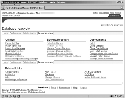
Figure 5.5 shows the Oracle Enterprise Manager Maintenance screen, from where you can launch the load wizard from the Utilities section. Click on the Load Data from File link. The wizard guides you through the process of loading data from an external file into the database according to a set of instructions in a control file and the subsequent submission of a batch job through Enterprise Manager to execute the load.
The control file is a text file that describes the load operation. The role of the control file, which is illustrated in Figure 5.6, is to tell SQL*Loader which datafile to load, how to interpret the records and columns, and into which tables to insert the data. At this point you also need to specify a host server account, which Enterprise Manager can use to execute your SQL*Loader job.
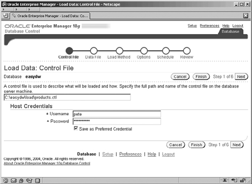
Hint
This is a server account and not the database account that you wish to use to access the tables that you’re loading into.
The control file is written in SQL*Loader’s data definition language. The following example shows the control file that would be used to add new product data into the product table in the EASYDW warehouse. The data is stored in the file product.dat. New rows will be appended to the existing table.
- Load product dimension
LOAD DATA
INFILE 'product.dat' append
INTO TABLE product
FIELDS TERMINATED BY ',' OPTIONALLY ENCLOSED BY "'"
(product_id,
 product_name,
 category,
 cost_price,
 sell_price,
 weight,
 shipping_charge,
 manufacturer,
 supplier)
The following example shows a small sample of the datafile product.dat. Each field is separated by a comma and optionally enclosed in a single quote. Each field in the input file is mapped to the corresponding columns in the table. As the data is read, it is converted from the data type in the input file to the data type of the column in the database.
'SP1242', 'CD LX1','MUSC', 8.90, 15.67, 2.5, 2.95, 'RTG', 'CD Inc'
'SP1243', 'CD LX2','MUSC', 8.90, 15.67, 2.5, 2.95, 'RTG', 'CD Inc'
'SP1244', 'CD LX3','MUSC', 8.90, 15.67, 2.5, 2.95, 'RTG', 'CD Inc'
'SP1245', 'CD LX4','MUSC', 8.90, 15.67, 2.5, 2.95, 'RTG', 'CD Inc'
The datafile is an example of data stored in Stream format. A record separator, often a line feed or carriage return/line feed, terminates each record. A delimiter character, often a comma, separates each field. The fields may also be enclosed in single or double quotes.
In addition to the Stream format, SQL*Loader supports fixed-length and variable-length format files. In a fixed-length file, each record is the same length. Normally, each field in the record is also the same length. In the control file, the input record is described by specifying the starting position, length, and data type. In a variable-length file, each record may be a different length. The first field in each record is used to specify the length of that record.
In OEM, the screen shown in Figure 5.7 is where the datafile is specified, and here it is c:easydwloadproducts.dat. The alternative mechanism to specify the data file location is within the control file, as shown previously by the INFILE parameter.
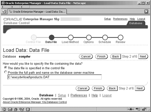
Figure 5.8 shows SQL*Loader’s three modes of operation:
Conventional path
Direct path
Parallel direct path

Conventional path load should only be used to load small amounts of data, such as initially loading a small dimension table or when loading data with data types not supported by direct path load. The conventional path load issues SQL INSERT statements. As each row is inserted, the indexes are updated, triggers are fired, and constraints are evaluated. When loading large amounts of data in a small batch window, direct path load can be used to optimize performance.
Direct path load bypasses the SQL layer. It formats the data blocks directly and writes them to the database files. When running on a system with multiple processors, the load can be executed in parallel, which can result in significant performance gains.
In the next step in the wizard, you are presented with the screen shown in Figure 5.9, which contains various options to control the execution of your SQL*Loader operation.
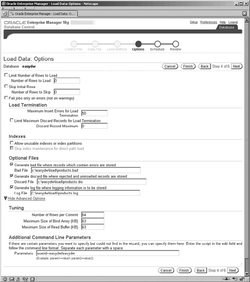
A common method when extracting datafiles from the source system is to have the first record in the file contain the names of the fields of the subsequent data records. This mechanism helps to self-document the datafile, which can be particularly useful when resolving errors for files with large and complex record formats. However, we do not want to have to manually remove this record prior to loading files of this format every single time this datafile is received. The Skip Initial Rows option will instruct SQL*Loader to do this removal for us automatically.
You can create additional files during the load operation to aid in the diagnosis and correction of any errors that may occur during the load. A log file is created to record the status of the load operation. This should always be reviewed to ensure the load was successful. Copies of the records that could not be loaded into the database because of data integrity violations can be saved in a “bad” file. This file can later be reentered once the data integrity problems have been corrected. If you receive an extract file with more records than you are interested in, you can load a subset of records from the file. The WHEN clause in the control file is used to select the records to load. Any records that are skipped are written to a discard file.
Select which optional files you would like created using the advanced option, as shown in Figure 5.9. In this example, we’ve selected a bad file, a discard file and a log file.
In order to specify the database account that SQL*Loader will log on with, you need to use the advanced options. Clicking on the Show Advanced Options link displays a hidden part of the page, where you can specify the account and password in the Parameters, field using the USERID parameter as shown.
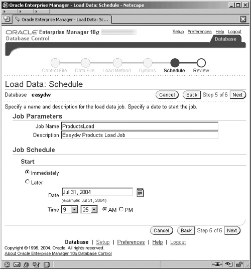
Enterprise Manager’s job scheduling system allows you to create and manage jobs, schedule the jobs to run, and monitor progress. You can run a job once or choose how frequently you would like the job to run. If you will run the job multiple times, you can save the job in Enterprise Manager’s jobs library so that it can be rerun in the future. In Figure 5.10, the job will be scheduled to run immediately. Click on Next and you will see the review screen (not shown) and clicking the Submit Job on this screen will actually submit your job for execution and display a status screen. At this point you will also have the option to monitor your job by clicking the View Job button which displays the screen shown in Figure 5.11 for monitoring your job.

You can also monitor the progress of a job while it is running by going to the bottom of the Administration screen and clicking on Jobs in the Related Links section. The Job Activity page shown in Figure 5.11 lists all jobs that are either running, are scheduled to run, or have completed.
The Results section contains a list of jobs and their status. You can check to see if the job ran successfully after it has completed and look at the output to see any errors when a job has failed. By selecting the job and clicking on the View or Edit buttons you can view information about the job’s state and progress, as shown in Figure 5.12.
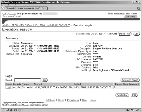
When SQL*Loader executes, it creates a log file, which can be inspected. The following example shows a log file from a sample load session that can be accessed by clicking on the Load name on the screen shown in Figure 5.12. The log file is also written to the file system (by default into the directory where the loader control file is held). Four rows were appended to the product table; one record was rejected due to invalid data. Copies of those bad records can be found in the file products.bad.
SQL*Loader: Release 10.1.0.2.0 - Production on Sat Jul 31 11:43:56 2004

Copyright (c) 1982, 2004, Oracle. All rights reserved.

Control File:   C:easydwloadproducts.ctl
Data File:      c:easydwloadproducts.dat
  Bad File:     C:easydwloadproducts.bad
  Discard File: none specified

 (Allow all discards)
Number to load: ALL
Number to skip: 0
Errors allowed: 50
Bind array:     64 rows, maximum of 64512 bytes
Continuation:    none specified
Path used:      Conventional

Table PRODUCT, loaded from every logical record.
Insert option in effect for this table: APPEND

Column Name                      Position   Len Term Encl Datatype
------------------------------ ---------- ----- ---- ---- --------
PRODUCT_ID                          FIRST     *   ,  O(') CHARACTER
PRODUCT_NAME                         NEXT     *   ,  O(') CHARACTER
CATEGORY                             NEXT     *   ,  O(') CHARACTER
COST_PRICE                           NEXT     *   ,  O(') CHARACTER
SELL_PRICE                           NEXT     *   ,  O(') CHARACTER
WEIGHT                               NEXT     *   ,  O(') CHARACTER
SHIPPING_CHARGE                      NEXT     *   ,  O(') CHARACTER
MANUFACTURER                         NEXT     *   ,  O(') CHARACTER
SUPPLIER                             NEXT     *   ,  O(') CHARACTER

value used for ROWS parameter changed from 64 to 27
Record 5: Rejected - Error on table PRODUCT, column PRODUCT_ID.
Column not found before end of logical record (use TRAILING
NULLCOLS)

Table PRODUCT:
  4 Rows successfully loaded.
  1 Row not loaded due to data errors.
  0 Rows not loaded because all WHEN clauses were failed.
  0 Rows not loaded because all fields were null.

Space allocated for bind array:        62694 bytes(27 rows)
Read buffer bytes:     64512

Total logical records skipped:              0
Total logical records read:                 5
Total logical records rejected:             1
Total logical records discarded:            0

Run began on Sat Jul 31 11:43:56 2004
Run ended on Sat Jul 31 11:43:56 2004

Elapsed time was:     00:00:00.66
CPU time was: 00:00:00.08When loading large amounts of data in a small batch window, a variety of techniques can be used to optimize performance:
Using direct path load. Formatting the data blocks directly and writing them to the database files eliminate much of the work needed to execute a SQL INSERT statement. Direct path load requires exclusive access to the table or partition being loaded. In addition, triggers are automatically disabled, and constraint evaluation is deferred until the load completes.
Disabling integrity constraint evaluation prior to loading the data. When loading data with direct path, SQL*Loader automatically disables all CHECK and REFERENCES integrity constraints. When using parallel direct path load or loading into a single partition, other types of constraints must be disabled. You can manually disable evaluation of not null, unique, and primary-key constraints during the load process as well. When the load completes, you can have SQL*Loader reenable the constraints, or do it yourself manually.
Loading the data in sorted order. Presorting data minimizes the amount of temporary storage needed during the load, enabling optimizations to minimize the processing during the merge phase to be applied. To tell SQL*Loader which indexes the data is sorted on, use the SORTED INDEXES statement in the control file.
Deferring index maintenance. Indexes are maintained automatically whenever data is inserted or deleted, or the key column is updated. When loading large amounts of data with direct path load, it may be faster to defer index maintenance until after the data is loaded. You can either drop the indexes prior to the beginning of the load or skip index maintenance by setting SKIP_INDEX_MAINTENANCE=TRUE on the SQL*Loader command line. Index partitions that would have been updated are marked “index unusable,” because the index segment is inconsistent with respect to the data it indexes. After the data is loaded, the indexes must be rebuilt separately.
Disabling redo logging by using the UNRECOVERABLE option in the control file. By default, all changes made to the database are also written to the redo log so they can be used to recover the database after failures. Media recovery is the process of recovering after the loss of a database file, often due to a hardware failure such as a disk head crash. By disabling redo logging, the load is faster.
However, if the system fails in the middle of loading the data, you need to restart the load, since you cannot use the redo log for recovery. If you are using Oracle Data Guard to protect your data with a logical or physical standby database, you may not want to disable redo logging. Any data not logged cannot be automatically applied to the standby site.
After the data is loaded, using the UNRECOVERABLE option, it is important to do a backup to make sure you can recover the data in the future if the need arises.
Loading the data into a single partition. While you are loading a partition of a partitioned or subpartitioned table, other users can continue to access the other partitions in the table. Loading the April transactions will not prevent users from querying the existing data for January through March. Thus, overall availability of the warehouse is increased.
Loading the data in parallel. When a table is partitioned, it can be loaded into multiple partitions in parallel. You can also set up multiple, concurrent sessions to perform a load into the same table or into the same partition of a partitioned table.
Increasing the STREAMSIZE parameter can lead to better direct path load times, since larger amounts of data will be passed in the data stream from the SQL*Loader client to the Oracle server.
If the data being loaded contains many duplicate dates, using the DATE_CACHE parameter can lead to better performance of direct path load. Use the date cache statistics (entries, hits, and misses) contained in the SQL*Loader log file to tune the size of the cache for future similar loads.
Next, we will look at an example of loading data into a single partition. In the EASYDW warehouse, the fact table is partitioned by date. At the end of April, the April sales transactions are loaded into the EASYDW warehouse.
In the following example, we create a tablespace, add a partition to the purchases table, and then use SQL*Loader direct path load to insert the data into the January 2005 partition.
CREATE TABLESPACE purchases_jan2005
 DATAFILE
  'C:ORACLEPRODUCT10.1.0ORADATAEASYDWPURCHASESJAN2005.f'
 SIZE 5M
 REUSE AUTOEXTEND ON
 DEFAULT STORAGE
  (INITIAL 64K NEXT 64K PCTINCREASE 0 MAXEXTENTS UNLIMITED);
If our new partition is higher than the last partition in the table (i.e., based on the boundary clauses), then we can add a partition, as follows:
ALTER TABLE easydw.purchases
      ADD PARTITION purchases_jan2005
      VALUES LESS THAN (TO_DATE('01-02-2005', 'DD-MM-YYYY'))
      PCTFREE 0 PCTUSED 99
      STORAGE (INITIAL 64K NEXT 64K PCTINCREASE 0)
TABLESPACE purchases_jan2005;When using direct path load of a single partition, referential and check constraints on the table partition must be disabled, along with any triggers.
SQL> ALTER TABLE purchases DISABLE CONSTRAINT fk_time;
SQL> ALTER TABLE purchases DISABLE CONSTRAINT fk_product_id;
SQL> ALTER TABLE purchases DISABLE CONSTRAINT fk_customer_id;
The status column in the USER_CONSTRAINTS view can be used to determine if the constraint is currently enabled or disabled. Here we can see that the special_offer constraint is still enabled.
SQL> SELECT TABLE_NAME, CONSTRAINT_NAME, STATUS
     FROM USER_CONSTRAINTS
     WHERE TABLE_NAME = 'PURCHASES';

TABLE_NAME    CONSTRAINT_NAME         STATUS
------------- ----------------------- --------
PURCHASES     NOT_NULL_PRODUCT_ID     DISABLED
PURCHASES     NOT_NULL_TIME           DISABLED
PURCHASES     NOT_NULL_CUSTOMER_ID    DISABLED
PURCHASES     SPECIAL_OFFER           ENABLED
PURCHASES     FK_PRODUCT_ID           DISABLED
PURCHASES     FK_TIME                 DISABLED
PURCHASES     FK_CUSTOMER_ID          DISABLED

7 rows selected.
The status column in the USER_TRIGGERS view can be used to determine if any triggers must be disabled. There are no triggers on the PURCHASES table.
SQL> SELECT TRIGGER_NAME, STATUS
     FROM ALL_TRIGGERS
     WHERE TABLE_NAME = 'PURCHASES';

no rows selectedThe following example shows the SQL*Loader control file to load new data into a single partition. Note that the partition clause is used.
OPTIONS (DIRECT=TRUE)
UNRECOVERABLE LOAD DATA
INFILE 'purchases.dat' BADFILE 'purchases.bad'
APPEND
INTO TABLE purchases
PARTITION (purchases_jan2005)
(product_id          position (1-6)    char,
 time_key            position (7-17)   date "DD-MON-YYYY",
 customer_id         position (18-25)  char,
 ship_date           position (26-36)  date "DD-MON-YYYY",
 purchase_price      position (37-43)  decimal external,
 shipping_charge     position (44-49)  integer external,
 today_special_offer position (50)     char)
The unrecoverable keyword is specified, disabling media recovery for the table being loaded by disabling the redo logging for this operation; this also necessitates that the DIRECT option be used as well. Database changes being made by other users will continue to be logged. After disabling media recovery, it is important to do a backup to make it possible to recover the data in the future if the need arises. If you attempted media recovery before the backup was taken, you would discover that the data blocks that were loaded have been marked as logically corrupt. To recover the data, if you haven’t performed the backup following the load operation, you would have to drop the partition and reload the data.
Any data that cannot be loaded will be written to the file purchases.bad. Data will be loaded into the PURCHASES_JAN2005 partition. This example shows loading a fixed-length file named purchases.dat. Each field in the input record is described by specifying the starting position, its ending position, and its data type. Note: These are SQL*Loader data types representing the data formats in the file, not the data types in an Oracle table. When the data is loaded into the tables, each field is converted to the data type of the Oracle table column, if necessary.
The following example shows a sample of the purchases data file. The PRODUCT_ID starts in column 1 and is six bytes long. “Time_key” starts in column 7 and is 11 bytes long. The data mask “DD-MON-YYYY” is used to describe the input format of the date fields.
12345678901234567890123456789012345678901234567890
      |          |       |          |      |     |
SP100001-jan-2005AB12367501-jan-20050067.23004.50N
SP101001-jan-2005AB12367301-jan-20050047.89004.50N
The alternative method to invoke SQL*Loader direct path mode is from the command line using DIRECT=TRUE. In this example, skip_index_ maintenance is set to true, so the indexes will need to be rebuilt after the load.
sqlldr USERID=easydw/easydw CONTROL=purchases.ctl
LOG=purchases.log DIRECT=TRUE SKIP_INDEX_MAINTENANCE=TRUE
The following example shows a portion of the SQL*Loader log file from the load operation. Rather than generating redo to allow recovery, invalidation redo was generated to let Oracle know this table cannot be recovered. The indexes were made unusable. The column starting position and length are described.
SQL*Loader: Release 10.1.0.2.0 - Production on Mon Jun 7 14:59:24 2004

Copyright (c) 1982, 2004, Oracle. All rights reserved.

Control File:   purchases.ctl
Data File:      purchases.dat
  Bad File:     purchases.bad
  Discard File:  none specified

 (Allow all discards)
Number to load: ALL
Number to skip: 0
Errors allowed: 50
Continuation:    none specified
Path used:      Direct

Load is UNRECOVERABLE; invalidation redo is produced.
Table PURCHASES, partition PURCHASES_JAN2005, loaded from every logical record.
Insert option in effect for this partition: APPEND
   Column Name                  Position   Len  Term Encl Datatype
------------------------------ ---------- ----- ---- ---- ---------------------
PRODUCT_ID                            1:6     6           CHARACTER
TIME_KEY                             7:17    11           DATE DD-MON-YYYY
CUSTOMER_ID                         18:25     8           CHARACTER
SHIP_DATE                           26:36    11           DATE DD-MON-YYYY
PURCHASE_PRICE                      37:43     7           CHARACTER
SHIPPING_CHARGE                     44:49     6           CHARACTER
TODAY_SPECIAL_OFFER                    50     1           CHARACTER

Record 3845: Discarded - all columns null.
The following index(es) on table PURCHASES were processed:
index EASYDW.PURCHASE_CUSTOMER_INDEX partition PURCHASES_JAN2005 was made unusable
due to:
SKIP_INDEX_MAINTENANCE option requested
index EASYDW.PURCHASE_PRODUCT_INDEX partition PURCHASES_JAN2005 was made unusable due
to:
SKIP_INDEX_MAINTENANCE option requested
index EASYDW.PURCHASE_SPECIAL_INDEX partition PURCHASES_JAN2005 was made unusable due
to:
SKIP_INDEX_MAINTENANCE option requested
index EASYDW.PURCHASE_TIME_INDEX partition PURCHASES_JAN2005 was made unusable due
to:
SKIP_INDEX_MAINTENANCE option requested
After loading the data into a single partition, all references to constraints and triggers must be reenabled. All local indexes for the partition can be maintained by SQL*Loader. Global indexes are not maintained on single partition or subpartition direct path loads and must be rebuilt. In the previous example, the indexes must be rebuilt since index maintenance was skipped.
These steps are discussed in more detail later in the chapter.
When a table is partitioned, the direct path loader can be used to load multiple partitions in parallel. Each parallel direct path load process should be loaded into a partition of a table stored on a separate disk to minimize I/O contention.
Since data is extracted from multiple operational systems, you will often have several input files that need to be loaded into the warehouse. These files can be loaded in parallel, and the workload distributed among several concurrent SQL*Loader sessions.
Figure 5.13 shows an example of how parallel direct path load can be used to initially load the historical transactions into the purchases table. You need to invoke multiple SQL*Loader sessions. Each SQL*Loader session takes a different datafile as input. In this example, there are three data files, each containing the purchases for one month: January, February, and March. These will be loaded into the purchases table, which is also partitioned by month. Each datafile is loaded in parallel into its own partition.
It is suggested that the following steps be followed to load data in parallel using SQL*Loader.
Constraints cannot be evaluated, and triggers cannot be fired during a parallel direct path load. If you forget, SQL*Loader will issue an error.
Indexes cannot be maintained during a parallel direct path load. However, if we are loading only a few partitions out of many, then it is probably better to skip index maintenance and have them marked as unusable instead.
By invoking multiple SQL*Loader sessions and setting direct and parallel to true, the processes will load concurrently. Depending on your operating system, you may need to put an “&” at the end of each line (i.e., to be able to invoke one sqlldr and immediately progress to invoking the second without waiting for number one to complete).
sqlldr userid=easydw/easydw CONTROL=jan.ctl DIRECT=TRUE PARALLEL=TRUE
sqlldr userid=easydw/easydw CONTROL=feb.ctl DIRECT=TRUE PARALLEL=TRUE
sqlldr userid=easydw/easydw CONTROL=mar.ctl DIRECT=TRUE PARALLEL=TRUE
A portion of one of the log files follows. Note that the mode is direct with the parallel option.
SQL*Loader: Release 10.1.0.2.0 - Production on Sat Jun 5 18:30:43 2004

Copyright (c) 1982, 2004, Oracle. All rights reserved.

Control File:   c:feb.ctl
Data File:      c:feb.dat
  Bad File:     c:feb.bad
  Discard File:  none specified

 (Allow all discards)

Number to load: ALL
Number to skip: 0
Errors allowed: 50
Continuation:    none specified
Path used:      Direct - with parallel option.

Load is UNRECOVERABLE; invalidation redo is produced.

Table PURCHASES, partition PURCHASES_FEB2004, loaded from every logical record.
Insert option in effect for this partition: APPENDAfter using parallel direct path load, reenable any constraints and triggers that were disabled for the load. Recreate any indexes that were dropped.
If you receive extract files that have data in them that you do not want to load into the warehouse, you can use SQL*Loader to filter the rows of interest. You select the records that meet the load criteria by specifying a WHEN clause to test an equality or inequality condition in the record. If a record does not satisfy the WHEN condition, it is written to the discard file. The discard file contains records that were filtered out of the load, because they did not match any record-selection criteria specified in the control file. Note that these records differ from rejected records written to the BAD file. Discarded records do not necessarily have any bad data. The WHEN clause can be used with either conventional or direct path load.
You can use SQL*Loader to perform simple types of transformations on character data. For example, portions of a string can be inserted using the substring function; two fields can be concatenated together using the CONCAT operator. You can trim leading or trailing characters from a string using the trim operator. The control file in the following example illustrates both the use of the WHEN clause to discard any rows where the PRODUCT_ID is blank and how to uppercase the PRODUCT_ID column.
LOAD DATA
INFILE 'product.dat' append
INTO TABLE product WHEN product_id != BLANKS
FIELDS TERMINATED BY ',' OPTIONALLY ENCLOSED BY "'"
(product_id "upper(:product_id)",
 product_name,
 category,
 cost_price,
 sell_price,
 weight,
 shipping_charge,
 manufacturer,
 supplier)
The discard file is specified when invoking SQL*Loader from the command line, as shown here, or with the OEM Load wizard, as seen previously.
sqlldr userid=easydw/easydw CONTROL=product.ctl
LOG=product.log BAD=product.bad DISCARD=product.dis DIRECT=true
These types of transformations can be done with both direct path and conventional path modes; however, since they are applied to each record individually, they do have an impact on the load performance.
After the data is loaded, you may need to process exceptions, reenable constraints, and rebuild indexes.
Always look at the logs to ensure that the data was loaded successfully. Validate that the correct number of rows have been added.
Look in the .bad file to find out which rows were not loaded. Records that fail NOT NULL constraints are rejected and written to the SQL*Loader bad file.
Ensure, referential integrity is reenabled, if you have not already done so. Make sure that each foreign key in the fact table has a corresponding primary key in each dimension table. For the EASYDW warehouse, each row in the PURCHASES table needs to have a valid CUSTOMER_ID in the CUSTOMERS table and a valid PRODUCT_ID in the PRODUCTS table.
When using direct path load, CHECK and REFERENCES integrity constraints were disabled. When using parallel direct path load, all constraints were disabled.
To find the rows with bad data, you can create an exceptions table. Create the table named “exceptions” by running the script UTLEXCPT.SQL. When enabling the constraint, list the table name the exceptions should be written to.
SQL> ALTER TABLE purchases
       ENABLE CONSTRAINT fk_product_id
       EXCEPTIONS INTO exceptions;
In our example, two rows had bad PRODUCT_IDs. A sale was made for a product that does not exist in the product dimension.
SQL> SELECT * FROM EXCEPTIONS;

ROW_ID             OWNER      TABLE_NAME  CONSTRAINT
------------------ ---------- ----------- -------------
AAAOZAAAkAAAABBAAB EASYDW     PURCHASES   FK_PRODUCT_ID
AAAOZAAAkAAAABBAAA EASYDW     PURCHASES   FK_PRODUCT_ID
To find out which rows have violated referential integrity, select the rows from the purchases table where the rowid is in the exception table. In this example, there are two rows where there is no matching product in the products dimension.
SQL> SELECT * from purchases WHERE rowid in (select row_id from
exceptions);

PRODUCT TIME_KEY  CUSTOMER_ID SHIP_DATE PURCHASE SHIPPING TODAY_SPECIAL
     ID                                    PRICE   CHARGE         OFFER
------- --------- ----------- --------- -------- -------- -------------
XY1001  01-JAN-05 AB123675    01-JAN-05    67.23      4.5 N
AB1234 01-JAN-05 AB123673 01-JAN-05 47.89 4.5 NIf integrity checking is maintained in an application, or the data has already been cleansed, and you know it will not violate any integrity constraints, enable the constraints with the NOVALIDATE clause. Include the RELY clause for query rewrite (which is discussed in Chapter 9). Since summary management and other tools depend on the relationships defined by referential integrity constraints, you should always define the constraints, even if they are not validated.
ALTER TABLE purchases ENABLE NOVALIDATE CONSTRAINT fk_product_id;
ALTER TABLE purchases MODIFY CONSTRAINT fk_product_id RELY;
Prior to publishing data in the warehouse, you should check to determine if any indexes are in an unusable state. An index becomes unusable when it no longer contains index entries to all the data. An index may be marked unusable for a variety of reasons.
You requested that index maintenance be deferred, using the skip_index_maintenance parameter when invoking SQL*Loader.
UNIQUE constraints were not disabled when using SQL*Loader direct path. At the end of the load, the constraints are verified when the indexes are rebuilt. If any duplicates are found, the index is not correct and will be left in an “Index Unusable” state.
The index must be dropped and recreated or rebuilt to make it usable again. If one partition is marked UNUSABLE, the other partitions of the index are still valid.
To check for unusable indexes query the table USER_INDEXES, as illustrated in the following code. Here we can see that the PRODUCT_PK_INDEX is unusable. If an index is partitioned, its status is N/A.
SQL> SELECT INDEX_NAME, STATUS FROM USER_INDEXES;

INDEX_NAME                    STATUS
------------------------------------
CUSTOMER_PK_INDEX             VALID
I_SNAP$_CUSTOMER_SUM          VALID
PRODUCT_PK_INDEX              UNUSABLE
PURCHASE_CUSTOMER_INDEX       N/A
PURCHASE_PRODUCT_INDEX        N/A
PURCHASE_SPECIAL_INDEX        N/A
PURCHASE_TIME_INDEX           N/A
TIME_PK_INDEX                 VALID
TSO_PK_INDEX                  VALID

9 rows selected.
Next, check to see if any index partitions are in an unusable state by checking the table USER_IND_PARTITIONS. In the following example, the PURCHASE_TIME_INDEX for the PURCHASES partitions for April, May, and June 2004 are unusable.
SQL> SELECT INDEX_NAME, PARTITION_NAME, STATUS FROM
     USER_IND_PARTITIONS WHERE STATUS != 'VALID';
INDEX_NAME                PARTITION_NAME       STATUS
------------------------- -------------------- --------
PURCHASE_TIME_INDEX       PURCHASES_MAR2004    USABLE
PURCHASE_TIME_INDEX       PURCHASES_APR2004    UNUSABLE
PURCHASE_TIME_INDEX       PURCHASES_MAY2004    UNUSABLE
PURCHASE_TIME_INDEX PURCHASES_JUN2004 UNUSABLEData Pump is a new product in Oracle Database 10g that enables a very rapid movement of data and metadata. In any data warehouse environment there will be the problem of transporting data from the source database to the warehouse database. When your source system is also on an Oracle Database 10g, then it makes sense to use the fast database import and export utilities to transport your data rather than resorting to character-based operating system files. The performance increase afforded by Data Pump import and export enables the necessary rapid transfer of data from one database to another, which is very important when moving the large volumes found when sourcing data for a warehouse. Data Pump reads and writes dump files in its own binary file format; this is in contrast to SQL*Loader, which can use files of different formats as defined by the control file.
If you have used the existing import and export utilities, imp and exp, then the new Data Pump import and export will be very familiar to you. However, in addition to the improved engine for shifting the data, they also provide a lot more functionality and control.
Hint
The dump files created and used by imp and exp cannot be used by the new Data Pump import and export.
The first, and most important, thing to note about Data Pump impdp and expdp is that they are client-side utilities, but the data movement is performed as a job running on the database that is accessing the dump file on the database host server directories. This detachment of the client utility from the server-side job means that more control, as well as independence, from the job is now available. For example, as a client-side tool, impdp and expdp no longer have to be dedicated to just one job on the server, but for long running jobs can, for example, detach from the job and re-attach, monitor and control a second job, or invoke a completely separate import/export operation.
Let’s have a brief look at the main new features of Data Pump impdp and expdp before working through an example of how they are used in our warehouse.
Restartability. The new utilities may stop and start the database server-side job. The new commands are STOP_JOB and START_JOB.
Attaching and detaching from a job. The client impdp and expdp can attach and detach from the database job, which provides a much needed improvement in the control over these potentially long-running operations.
Performing a network import. A new parameter, NETWORK_LINK, when used on an import, instructs a local database to access a remote database, retrieve data from it, and insert it into the local database.
Performing a network export. On export operations, NETWORK_LINK allows data from a remote database to be written to dump files on the local database server.
Mapping of datafile names. For import operations it is now possible to control the transformation of a datafile name on the source database to a different datafile name on the import database. Of particular importance, this feature can be used to change the file name formats used by different operating systems.
Remapping of tablespaces during import.
Filtering the objects that are exported and imported. Two new parameters are provided, called INCLUDE and EXCLUDE, which enable specification of the type of object and also control over the name of the objects.
Filtering the data that is exported. By using the Data Pump QUERY parameter, a subset of the data can be exported via a WHERE clause.
The ability to estimate the space an export job would use prior to performing the export.
The ability to use multiple dump files.
To control the degree of parallelism by use of the PARALLEL parameter. If multiple dump files are used, then it is normal for PARALLEL to be set to the number of the files.
Before using Data Pump, a directory object must be created in the database to specify the location of the dump files and log files. The dump and log files must be on the same machine as the database server, or must be accessible to the server (i.e., on a networked drive). This is different from SQL*Loader, where the SQL*Loader client sends the data to the database server. Directories are created in a single namespace and are not owned by an individual’s schema. In the following example, the DBA creates directories for the data and log files.
CREATE OR REPLACE DIRECTORY data_file_dir AS 'C:datafiles';
CREATE OR REPLACE DIRECTORY log_file_dir AS 'C:logfiles';
Read and write access must be granted to the users that will be accessing the dump files in the directory. In the example below, the DBA grants read and write access to user easydw.
GRANT READ, WRITE ON DIRECTORY data_file_dir TO easydw;
GRANT READ, WRITE ON DIRECTORY log_file_dir TO easydw;
To find the directories defined in a database, check the DBA_DIRECTORIES view.
SELECT * FROM DBA_DIRECTORIES;

OWNER        DIRECTORY_NAME          DIRECTORY_PATH
------------ ----------------------- ---------------
SYS          LOG_FILE_DIR            c:logfiles
SYS          DATA_FILE_DIR           c:datafiles
Suppose we want to export all of the OLTP ORDERS data for December 2004 from our OLTP database and move it to our warehouse database. Let us create a job to export the data using the new Data Pump export utility. We will use a parameter file called expdp_par.txt for this, which will contain all of the command-line arguments.
Hint
It is advisable to use a parameter file when the command contains keywords with values that contain spaces or quoted strings, such as QUERY and INCLUDE.
SCHEMAS=(OLTP)
INCLUDE=TABLE:"IN ('ORDERS')"
QUERY=OLTP.ORDERS:"WHERE purchase_date BETWEEN to_date('01-dec-
2004','dd-mon-yyyy') AND to_date('31-dec-2004','dd-mon-yyyy')"
DIRECTORY=data_file_dir
DUMPFILE=exp1.dmp
LOGFILE=log_file_dir:exporders2004.log
The QUERY clause allows us to specify a WHERE clause to filter the data. If the source table ORDERS were partitioned by date with a partition for each month, an alternative method to using the QUERY parameter would be to use the TABLES clause to specify the partition, as shown here.
TABLES=OLTP.ORDERS:DEC04 where DEC04 is the name of the partition.
Now we launch Data Pump export with the following command:
expdp oltp/oltp@easydw parfile=expdp_par.txt
The output at the start of the expdp execution is shown below:
Export: Release 10.1.0.2.0 - Production on Thursday, 08 July, 2004
21:11

Copyright (c) 2003, Oracle. All rights reserved.

Connected to: Oracle Database 10g Enterprise Edition Release
10.1.0.2.0 - Production
With the Partitioning, OLAP and Data Mining options
FLASHBACK automatically enabled to preserve database integrity.
Starting "OLTP"."SYS_EXPORT_SCHEMA_01": oltp/********@easydw
parfile=expdp_par.txt
Estimate in progress using BLOCKS method...
Processing object type SCHEMA_EXPORT/TABLE/TABLE_DATA
Total estimation using BLOCKS method: 64 KB
Processing object type SCHEMA_EXPORT/TABLE/PROCACT_INSTANCE
Processing object type SCHEMA_EXPORT/TABLE/TABLE
Processing object type SCHEMA_EXPORT/TABLE/CONSTRAINT/CONSTRAINT
Processing object type SCHEMA_EXPORT/TABLE/STATISTICS/
TABLE_STATISTICS
Here we can see that the Data Pump export will automatically use the new Oracle Database 10g Flashback capability of the database to preserve the integrity of our exported data. Flashback is part of a much larger feature in Oracle Database 10g that enables earlier versions of the data to be retrieved by rewinding the view of the data to an earlier point in time. We will look at Flashback in more detail in Chapter 17 but for our export, Data Pump is using Flashback to maintain a consistent view of the data at the point where we issued the expdp command.
This should not be confused with the Data Pump export parameter called FLASHBACK_TIME that enables export of data that is consistent with an earlier point in time.
Another new item to note in the output from Data Pump export is that an estimate of the export file size is provided for each of the tables exported. There are two mechanisms that are used, BLOCKS and STATISTICS, which are specified by the ESTIMATE parameter. Associated with this, there is also the ability to cap the size of the generated dump file using the FILESIZE parameter.
Now that we have exported our data, we can move the dump file exp1.dmp between our source server and our warehouse server using any conventional means such as FTP.
On the warehouse server, we must now import the data using impdp. Let’s look at some new options that are available to us. During the import we may want to put our source data in a different tablespace to keep it separated from the tablespaces that we are using for our warehouse tables. We do this using the REMAP_TABLESPACE parameter, which is used to specify the mapping between the tablespace on the source system (USERS) and the tablespace on the warehouse (STAGE).
Similarly, we want to change the ownership of the table from the OLTP account on the source system to the EASYDW account on the warehouse, and this mapping is specified using the REMAP_SCHEMA parameter.
impdp easydw/easydw@easydw DIRECTORY=data_file_dir
DUMPFILE=exp1.dmp
LOGFILE=log_file_dir:imporders2004.log
REMAP_TABLESPACE=users:stage REMAP_SCHEMA=oltp:easydw
In the same fashion that the control can be exercised over what is exported by Data Pump export, import also has the same facility to control the type of metadata this is imported. For example, by using the EXCLUDE=GRANT parameter and keyword during Data Pump import, it is possible to exclude object grants from being imported. In this way, Data Pump import will not try to regrant privileges that were only valid on the source database.
Let’s look in more detail at the new improvements to monitoring and controlling our import and export jobs that the new impdp and expdp provide.
In Oracle Database 10g, impdp and expdp are client-side tools that communicate with a database server-side job that is actually doing the import and export. This provides the opportunity for the client to attach to the job that is running on the database, monitor its status, suspend it or alter some of its execution parameters, detach from it and reattach, and monitor and control another job. This provides a lot more flexibility over the preceding imp and exp utilities. Note that impdp and expdp can only be attached and control; one server-side job at a time; however, you can have multiple impdp/expdp clients running—each of which can be attached to the same or different server-side jobs.
When these tools are running in normal noninteractive mode, you can move into interactive mode by typing Control-C.
In interactive mode, the commands that we can issue are:
ADD_FILE to add a new dump file for the export
KILL_JOB to delete the job
STOP_JOB, which will suspend the processing of our job and exit back to the operating system
PARALLEL to alter the degree of parallelism
If we want to reconnect Data Pump export to a suspended job, then we can reinvoke expdp with the ATTACH command-line parameter. If we originally provided our export job with a job name (e.g., JOB_NAME=expfull), then we can specifically name the job that we want to attach to. If there is only one job executing for the database account, then Data Pump export will automatically attach to it.
An example of this activity is shown in the following code. We are running Data Pump export using the JOB_NAME=expfull parameter.
C:> expdp easydw/easydw@easydw full=y directory=data_file_dir dumpfile=
full_dump.dat job_name=expfull

Export: Release 10.1.0.2.0 - Production on Saturday, 10 July, 2004 10:32

Copyright (c) 2003, Oracle. All rights reserved.

Connected to: Oracle Database 10g Enterprise Edition Release 10.1.0.2.0 - Production
With the Partitioning, OLAP and Data Mining options
FLASHBACK automatically enabled to preserve database integrity.
Starting "EASYDW"."EXPFULL": easydw/********@easydw full=y directory=data_file_dir
dumpfile=full_dump.dat job_name=expfull
Estimate in progress using BLOCKS method...
                                     ← Issue a Control-C here
Export> stop_job=immediate
Are you sure you wish to stop this job ([y]/n): y
                                     ← Returned to the operating system


C:easydwdp>expdp easydw/easydw@easydw attach=expful← Restart expdp and name
                                                         the job to attach to
Export: Release 10.1.0.2.0 - Production on Saturday, 10 July, 2004 10:32

Copyright (c) 2003, Oracle. All rights reserved.

Connected to: Oracle Database 10g Enterprise Edition Release 10.1.0.2.0 - Production
With the Partitioning, OLAP and Data Mining options

Job: EXPFULL                  ← Automatic report of the job status when we attach
  Owner: EASYDW
  Operation: EXPORT
  Creator Privs: FALSE
  GUID: F3A0628C541B4DD5B35F34C164A8408A
  Start Time: Saturday, 10 July, 2004 10:32
  Mode: FULL
  Instance: easydw
  Max Parallelism: 1
  EXPORT Job Parameters:
  Parameter Name      Parameter Value:
     CLIENT_COMMAND        easydw/********@easydw full=y directory=data_file_dir
 dumpfile=full_dump.dat job_name=expfull
     DATA_ACCESS_METHOD    AUTOMATIC
     ESTIMATE              BLOCKS
     INCLUDE_METADATA      1
     LOG_FILE_DIRECTORY    DATA_FILE_DIR
     LOG_FILE_NAME         export.log
     TABLE_CONSISTENCY     0
  State: IDLING
  Bytes Processed: 0
  Current Parallelism: 1
  Job Error Count: 0
  Dump File: c:easydwexternalfull_dump.dat
    bytes written: 4,096

Worker 1 Status:
  State: UNDEFINED

Export> continue_client      ← Restart the job and the logging.
                                 Return to non-interactive mode
Job EXPFULL has been reopened at Saturday, 10 July, 2004 10:32
Restarting "EASYDW"."EXPFULL": easydw/********@easydw full=y
directory=data_file_dir dumpfile=full_dump.dat job_name=expfull
Estimate in progress using BLOCKS method...
Processing object type DATABASE_EXPORT/SCHEMA/TABLE/TABLE_DATA
                                   ← Issue a Control-C here
Export> stop_job=immediate
Are you sure you wish to stop this job ([y]/n): y
We have only touched upon some of the new, powerful features available with Data Pump import and export, but it should be apparent that the features provided are very important in a warehouse environment when dealing with large data volumes. There are three main areas that benefit our warehouse management from the new Data Pump import and export utilities:
The significantly improved speed and performance from the new Data Pump architecture used to move the data in and out of the database
The new parameters, which provide additional control of the import and export jobs
The new client architecture and commands, which provide better monitoring and management of the jobs
An external table is a table stored outside the database in a flat file. The data in an external table can be queried just like a table stored inside the database. You can select columns, rows, and join the data to other tables using SQL. The data in the external table can be accessed in parallel just like tables stored in the database.
External tables are read-only. No DML operations are allowed, and you cannot create indexes on an external table. If you need to update the data or access it more than once, you can load it into the database, where you can update it and add indexes to improve query performance. By loading the data into the database, you can manage it as part of the database. RMAN will not back up the data for any external tables that are defined in the database.
Since you can query the data in the external table you have just defined using SQL, you can also load the data using an INSERT SELECT statement. External tables provide an alternative to SQL*Loader to load data from flat files. They can be used to perform more complex transformations while the data is loaded and simplify many of the operational aspects while loading data in parallel and managing triggers, constraints, and indexes. However, in Oracle Database 10g, SQL*Loader direct path load may still be faster in many cases. There are many similarities between the two methods, and if you’ve used SQL*Loader, you will find it easy to learn to use external tables.
External tables require the same directory objects that we defined in earlier.
In order to create an external table you must specify the following:
The metadata, which describes how the data looks to Oracle, including the external table name, the column names, and Oracle data types. These are the names you will use in the SQL statements to access the external table. The metadata is stored in the Oracle data dictionary. In the example in Figure 5.14, the external table name is NEW_PRODUCTS. The data is stored outside the database. This differs from the other regular tables in the database, where the data and metadata are both stored in the database.
The access parameters, which describe how the data is stored in the external file (i.e., where it’s located, its format, and how to identify the fields and records). The access driver uses the access parameters. An example of the access parameters is shown in the CREATE EXTERNAL TABLE statement.
In Oracle 9i, there was only one type of access driver, called ORACLE_LOADER, which provides read-only access to flat files. In Oracle Database 10g, a new ORACLE_DATAPUMP access driver is introduced; provides greater performance, as we have already discussed, and new features, which we will discuss later. The access driver is specified in the TYPE clause on the CREATE EXTERNAL TABLE statement.
The following example shows the SQL to create an external table. In the CREATE TABLE statement, the ORGANIZATION EXTERNAL clause is used to specify the table as external, and the TYPE clause to specify the type of access driver and which begins the description of the structure of the file stored on disk. The metadata describing the column names and data types is listed and looks very similar to what is stored in a SQL*Loader control file. The locations of the datafile, log file, and bad files are specified here, and in this example we specify that each field be separated by a comma and optionally enclosed in a single quote. By specifying the PARALLEL clause, the data will be loaded in parallel.
CREATE TABLE new_products
(product_id             VARCHAR2(8),
 product_name           VARCHAR2(30),
 category               VARCHAR2(4),
 cost_price             NUMBER (6,2),

 sell_price             NUMBER (6,2),
 weight                 NUMBER (4,2),
 shipping_charge        NUMBER (5,2),
 manufacturer           VARCHAR2(20),
 supplier               VARCHAR2(10))
ORGANIZATION EXTERNAL
(TYPE ORACLE_LOADER
   DEFAULT DIRECTORY data_file_dir
   ACCESS PARAMETERS
        (RECORDS DELIMITED BY NEWLINE
         CHARACTERSET US7ASCII
         BADFILE log_file_dir:'product.bad'
         LOGFILE log_file_dir:'product.log'
         FIELDS TERMINATED BY ','
                OPTIONALLY ENCLOSED BY "'")
   LOCATION  ('product.dat')
)
REJECT LIMIT UNLIMITED PARALLEL;
A portion of the data file, product.dat is shown in the following example. Each field is separated by a comma and optionally enclosed in a single quote. As the data is read, each field in the input file is mapped to the corresponding columns in the external table definition. As the data is read, it is converted from the data type of the input file to the data type of the column in the database, as necessary.
'SP1000', 'Digital Camera','ELEC', 45.67, 67.23, 15.00, 4.50, 'Ricoh','Ricoh'
'SP1001', 'APS Camera','ELEC', 24.67, 36.23,5.00, 4.50, 'Ricoh','Ricoh'
'SP1010', 'Camera','ELEC', 35.67, 47.89, 5.00,4.50, 'Agfa','Agfa'
After executing the CREATE TABLE command shown previously, the metadata for the NEW_PRODUCTS table is stored in the database. The table is as follows:
SQL> DESCRIBE new_products;

 Name                  Null?    Type
 --------------------- -------- -------------
 PRODUCT_ID                     VARCHAR2(8)
 PRODUCT_NAME                   VARCHAR2(30)
 CATEGORY                       VARCHAR2(4)
 COST_PRICE                     NUMBER(6,2)
 SELL_PRICE                     NUMBER(6,2)
 WEIGHT                         NUMBER(4,2)
 SHIPPING_CHARGE                NUMBER(5,2)
 MANUFACTURER                   VARCHAR2(20)
 SUPPLIER                       VARCHAR2(10)
The USER_EXTERNAL_TABLES dictionary view shows which external tables have been created, along with a description of them. The USER_EXTERNAL_LOCATIONS dictionary view shows the location of the datafile.
SQL> SELECT * FROM USER_EXTERNAL_TABLES;

TABLE_NAME      TYPE_OWNER TYPE_NAME
--------------- ---------- ------------------------------
DEFAULT_DIRECTORY_OWNER DEFAULT_DIRECTORY_NAME
----------------------- ------------------------------
REJECT_LIMIT                             ACCESS_TYPE
---------------------------------------- -----------
ACCESS_PARAMETERS
-----------------------------------------------------------
PROPERTY
----------
NEW_PRODUCTS    SYS        ORACLE_LOADER
SYS                     DATA_FILE_DIR
UNLIMITED                               CLOB
RECORDS DELIMITED BY NEWLINE
       CHARACTERSET US7ASCII
       BADFILE log_file_dir:'product.bad'
       LOGFILE log_file_dir:'product.log'
       FIELDS TERMINATED BY ',' OPTIONALLY ENCLOSED BY "'"
ALL

SQL> SELECT * FROM USER_EXTERNAL_LOCATIONS;

TABLE_NAME    LOCATION DIR DIRECTORY_NAME
------------- ------------ --- ------------
NEW_PRODUCTS product.dat SYS DATA_FILE_DIRAfter defining the external table, it can be accessed using SQL, just as if it were any other table in the database, although the data is actually being read from the file outside the database. A portion of the output is as follows:
SQL> SELECT * FROM NEW_PRODUCTS;

PRODUCT PRODUCT_NAME    CATE  COST  SELL  WEIGHT SHIPPING MANUF SUPPLIER
ID                           PRICE PRICE           CHARGE
------- --------------- ---- ----- ----- ------- -------- ----- --------
SP1000  Digital  Camera ELEC 45.67 67.23      15      4.5 Ricoh Ricoh
SP1001  APS  Camera     ELEC 24.67 36.23       5      4.5 Ricoh Ricoh
SP1010  Camera          ELEC 35.67 47.89       5      4.5 Agfa Agfa
The next example will use the INSERT/SELECT statement to load the data into the PRODUCT dimension table. It is very easy to perform transformations during the load using SQL functions and arithmetic operators. In this example, after the datafile was created, the cost of fuel rose, and our shipping company increased the shipping rates by 10 percent. In this example, data is loaded into the EASYDW.PRODUCT table by selecting the columns from the NEW_PRODUCTS external table. The shipping charge is multiplied by 1.1 for each item as the data is loaded.
SQL> INSERT INTO easydw.product
       (product_id, product_name, category,
        cost_price, sell_price, weight,
        shipping_charge, manufacturer, supplier)
     SELECT product_id, product_name, category,
            cost_price, sell_price, weight,
            (shipping_charge * 1.10),
            manufacturer, supplier
     FROM new_products;
The data has now been loaded into the EASYDW.PRODUCT table, and we can see here that the shipping charge increased from $4.50 to $4.95 for the items displayed.
SQL> select * from easydw.product;

PRODUCT PRODUCT_NAME    CATE  COST  SELL  WEIGHT SHIPPING MANUF SUPPLIER
ID                           PRICE PRICE           CHARGE
------- --------------- ---- ----- ----- ------- -------- ----- --------
SP1000  Digital  Camera ELEC 45.67 67.23      15     4.95 Ricoh    Ricoh
SP1001  APS  Camera     ELEC 24.67 36.23       5     4.95 Ricoh    Ricoh
SP1010  Camera          ELEC 35.67 47.89       5     4.95  Agfa     Agfa
Another advantage of using external tables is the ability to load the data in parallel without having to split a large file into smaller files and start multiple sessions, as you must do with SQL*Loader. The degree of parallelism is set using the standard parallel hints or with the PARALLEL clause when creating the external table, as shown previously. The output of an EXPLAIN PLAN shows the parallel access, as follows:
SQL> EXPLAIN PLAN FOR
     INSERT INTO easydw.product
         (product_id, product_name, category,
         cost_price, sell_price, weight,
         shipping_charge, manufacturer, supplier)
     SELECT product_id, product_name, category,
            cost_price, sell_price, weight,
            (shipping_charge * 1.10),
            manufacturer, supplier
     FROM new_products;
The utlxplp.sql script is used to show the EXPLAIN PLAN output with the columns pertaining to parallel execution, which have been edited and highlighted for readability. Chapter 10 provides more of an explanation on how to read parallel execution plans.
SQL> @c:oracleproduct10.1.0db_1
dbmsadminutlxplp.sql

PLAN_TABLE_OUTPUT
----------------------------------------------------------------------------------------------

----------------------------------------------------------------------------------------------
| Id  | Operation                     | Name         | Rows  | Bytes | Cost (%CPU)| Time     |
----------------------------------------------------------------------------------------------
|   0 | INSERT STATEMENT              |              |  8168 |   781K|    13   (0)| 00:00:01 |
|   1 |  PX COORDINATOR               |              |       |       |            |          |
|   2 |   PX SEND QC (RANDOM)         | :TQ10000     |  8168 |   781K|    13   (0)| 00:00:01 |
|   3 |    PX BLOCK ITERATOR          |              |  8168 |   781K|    13   (0)| 00:00:01 |
|   4 |     EXTERNAL TABLE ACCESS FULL| NEW_PRODUCTS |  8168 |   781K|    13   (0)| 00:00:01 |
----------------------------------------------------------------------------------------------Data Pump external tables are another fast method available to us for moving data between databases; now we can actually write to the external file during the creation of the external table, which we could not do with the ORACLE_LOADER access driver. We will demonstrate this with an example.
First, let’s create our external table based on the current PURCHASES table. To do this we will use a database directory object called xt_dir, where our external data file, called purch_xt.dmp, will reside.
CREATE TABLE purchases_xt ORGANIZATION EXTERNAL
( TYPE ORACLE_DATAPUMP
  DEFAULT DIRECTORY xt_dir
  LOCATION ('purch_xt.dmp')
)
AS SELECT * FROM purchases;
This statement is creating the Data Pump dump file, purch_xt.dmp, as the external table PURCHASES_XT is being created. Once it has been created, you can select from this table just like any other however, because it is now an external table, after the initial CREATE statement it is not possible to perform any further alterations to the records. Any subsequent DELETE, INSERT or UPDATE operations will result in an Oracle error, as illustrated here.
SQL> desc purchases_xt
 Name                       Null?    Type
 -------------------------- -------- -----------------------
 PRODUCT_ID                 NOT NULL VARCHAR2(8)
 TIME_KEY                   NOT NULL DATE
 CUSTOMER_ID                NOT NULL VARCHAR2(10)
 SHIP_DATE                           DATE
 PURCHASE_PRICE                      NUMBER(6,2)
 SHIPPING_CHARGE                     NUMBER(5,2)
 TODAY_SPECIAL_OFFER                 VARCHAR2(1)

SQL> SELECT count(*) FROM purchases_xt;

  COUNT(*)
----------
     94619

SQL> SELECT * FROM purchases_xt WHERE rownum < 3;


PRODUCT  TIME_KEY  CUSTOMER_I SHIP_DATE PURCHASE SHIPPING T
ID                                         PRICE   CHARGE
-------- --------- ---------- --------- -------- -------- -
SP1001   01-JAN-03 AB123899   01-JAN-03    36.23      4.5 N
SP1011   01-JAN-03 AB123897   01-JAN-03    47.89      4.5 N

SQL> UPDATE purchases_xt SET purchase_price=37 WHERE
product_id='SP1001';
UPDATE purchases_xt SET purchase_price=37 WHERE
product_id='SP1001'
       *
ERROR at line 1:
ORA-30657: operation not supported on external organized table
We can now move this Data Pump formatted dump file from our specified directory to another server and access it from another database to use it as the basis of a new external table. This time, however, to create our external table we will need to specify the columns explicitly, as shown here.
CREATE TABLE purchases_xt2
 (product_id          VARCHAR2(8) ,
  time_key            DATE ,
  customer_id         VARCHAR2(10) ,
  ship_date           DATE,
  purchase_price      NUMBER(6,2),
  shipping_charge     NUMBER(5,2),
  today_special_offer VARCHAR2(1)
 )
 ORGANIZATION EXTERNAL
 (
  TYPE ORACLE_DATAPUMP
  DEFAULT DIRECTORY xt_dir
  LOCATION ('purch_xt.dmp')
 );

Table created.

SQL> SELECT count(*) FROM purchases_xt2;

  COUNT(*)
----------
     94619
By using a Data Pump external table, we have reaped the benefit of the performance improvements from Data Pump for both the writing of the dump file and also the reading of it on the target database. In addition, the syntax of the commands for creating this version of an external table is very succinct and readable.
Because the creation of the initial external table and the dump file can use a CREATE TABLE AS SELECT operation, we also have the capability to perform filtering with a WHERE clause and use joins when the external table is created. This can form a powerful mechanism for being selective and controlling the data that is transferred to the external table. For example, for transferring the data from a refreshed warehouse schema into a data mart, which requires a smaller subset of the fact data, the data is filtered with a WHERE clause when the external table is created.
The fastest way to move data from one Oracle database to another is using transportable tablespaces. Transportable tablespaces provide a mechanism to move one or more tablespaces from one Oracle database into another. Rather than processing the data a row at time, the entire file or set of files is physically copied from one database and integrated into the second database by importing the metadata describing the tables from the files themselves. In addition to data in tables, the indexes can also be moved.
Because the data is not unloaded and reloaded, just detached, it can be moved quickly. In Oracle 9i, you could only transport tablespaces between Oracle databases that were on the same operating system. In Oracle Database 10g, this limitation is removed, and transportable tablespaces can be moved between different operating system platforms—for example, from Windows to Linux.
Transportable tablespaces can be used to move data from the operational database to the staging area if you are using an Oracle database to do your staging. Transportable tablespaces are also useful to move data from the data warehouse to a dependent data mart.
Figure 5.15 shows the steps involved in using transportable tablespaces.
These steps are as follows:
Create a new tablespace.
Move the data you want to transfer into its own tablespace.
Alter the tablespace to read-only.
Use the export utility to unload the metadata describing the objects in the tablespace.
If moving between different operating systems, then convert the files using RMAN (this conversion step can alternatively be performed on the target platform after step 6).
Copy the datafiles and export dump file containing the metadata to the target system.
Use the import utility to load the metadata descriptions into the target database.
Alter the tablespace to read/write.
Perform transformations.
Move the data from the staging area to the warehouse fact table.

This section will discuss steps 1–8. In the following sections, we’ll look at steps 9 and 10.
One of the sources for data in the EASYDW Warehouse is an Oracle Database 10g order-entry system. In this example, the order-entry system has a record for every order stored in the ORDERS table. At the end of April, all the orders for April 2004 will be copied into a new table, called APR_ORDERS, in the ORDERS tablespace stored in the datafile “orders.f.”
Here are the steps that are required to transport a tablespace from one database to another. In our example, our source OLTP system is on Linux and our target warehouse system is on a Windows platform.
Choose a name that is unique on both the source and target system. In this example, the tablespace ORDERS is created, and its corresponding datafile is “orders.f.”
SQL> CREATE TABLESPACE orders
     DATAFILE 'C:ORACLEPRODUCT10.1.0ORADATAEASYDWorders.f'
     SIZE 5M REUSE
     AUTOEXTEND ON
     DEFAULT STORAGE
(INITIAL 64K PCTINCREASE 0 MAXEXTENTS UNLIMITED);In this example, a table is created and populated using the CREATE TABLE AS SELECT statement. It is created in the ORDERS tablespace. In this example, there are 3,720 orders for April.
SQL> CREATE TABLE oltp.apr_orders TABLESPACE orders
     AS
     SELECT * FROM purchases
     WHERE ship_date BETWEEN to_date('01-APR-2004', 'dd-on-yyyy')
                        AND to_date('30-APR-2004', 'dd-mon-yyyy'),

SQL> SELECT COUNT(*) FROM apr_orders;

  COUNT(*)
----------
      3720
Each tablespace must be self-contained and cannot reference anything outside the tablespace. If there were a global index on the April ORDERS table, it would not be self-contained, and the index would have to be dropped before the tablespace could be moved.
If you do not do this, the export in the next step will fail.
SQL> ALTER TABLESPACE orders READ ONLY;
By using the Data Pump expdp command, the metadata definitions for the orders tablespace are extracted and stored in the export dump file “expdat.dmp.”
expdp system/manager TRANSPORT_TABLESPACE=orders
DIRECTORY=data_file_dir
DUMPFILE=expdat.dmp
When transporting a set of tablespaces, you can choose to include referential integrity constraints. However, if you do include these, you must move the tables with both the primary and foreign keys.
Hint
When exporting and importing tablespaces, be sure to use an account that has been granted the EXP_FULL_DATABASE role.
The following code is a copy of the run-time information generated by the export. Only the tablespace metadata is exported, not the data.
$ expdp system/magic9 transport_tablespaces=orders
directory=data_file_dir dumpfile=expdat.dmp

Export: Release 10.1.0.2.0 - Production on Saturday, 10 July, 2004 8:01

Copyright (c) 2003, Oracle. All rights reserved.

Connected to: Oracle Database 10g Enterprise Edition Release 10.1.0.2.0 - Production
With the Partitioning, OLAP and Data Mining options
Starting "SYSTEM"."SYS_EXPORT_TRANSPORTABLE_01": system/********
transport_tablespaces=orders directory=data_file_dir dumpfile=expdat.dmp
Processing object type TRANSPORTABLE_EXPORT/PLUGTS_BLK
Processing object type TRANSPORTABLE_EXPORT/TABLE
Processing object type TRANSPORTABLE_EXPORT/TABLE_STATISTICS
Processing object type TRANSPORTABLE_EXPORT/TTE_POSTINST/PLUGTS_BLK
Master table "SYSTEM"."SYS_EXPORT_TRANSPORTABLE_01" successfully
loaded/
unloaded****************************************************************************
**
Dump file set for SYSTEM.SYS_EXPORT_TRANSPORTABLE_01 is:
  /home/oracle/tt/expdat.dmp
Job "SYSTEM"."SYS_EXPORT_TRANSPORTABLE_01" successfully completed at 08:04
If you are transporting between different platforms and the endian formats of your platforms are different, you will need to convert the data files. The endian nature of your platform is the format in which multibyte data is stored. Big endian platforms store the most significant byte in the lowest address and little endian platforms store it in the highest address.
Oracle provides some tables and a simple query to determine the endian nature of your source and target platforms.
SELECT d.PLATFORM_NAME, tp.ENDIAN_FORMAT
FROM   V$TRANSPORTABLE_PLATFORM tp,
       V$DATABASE d
WHERE  tp.PLATFORM_NAME = d.PLATFORM_NAME;
When the query is run on the source Linux platform database, we see that the platform uses little endian format.
PLATFORM_NAME                            ENDIAN_FORMAT
---------------------------------------- --------------
Linux IA (32-bit)                        Little
When the query is run on the target warehouse database, we see that it is also little endian.
PLATFORM_NAME                            ENDIAN_FORMAT
---------------------------------------- --------------
Microsoft Windows IA (32-bit)            Little
If the endian format were different on the two platforms, then conversion would be required. In our example, even though both of our platforms are of the same endian format, we will still demonstrate the step for the conversion, which uses the Recovery Manager utility RMAN.
$ rman target /

Recovery Manager: Release 10.1.0.2.0 - Production
 Copyright (c) 1995, 2004, Oracle. All rights reserved.
 connected to target database: ORCL (DBID=1058909169)

RMAN> convert tablespace orders
2> to platform 'Microsoft Windows IA (32-bit)'
3> FORMAT '/home/oracle/tt/%N_%f' ;
Starting backup at 10-JUL-04
using target database controlfile instead of recovery catalog
allocated channel: ORA_DISK_1
channel ORA_DISK_1: sid=244 devtype=DISK
channel ORA_DISK_1: starting datafile conversion
input datafile fno=00005 name=/u01/app/oracle/oradata/orcl/
orders.f
converted datafile=/home/oracle/tt/ORDERS_5
channel ORA_DISK_1: datafile conversion complete, elapsed time:
00:00:01
Finished backup at 10-JUL-04
The conversion format mask ′%N_%f′ that was used will create a file name in the directory specified using the original tablespace name (%N) and the file id number on the database (%f).
If the conversion is performed on the source system, then RMAN can reference the tablespaces by logging on to the database, but if the conversion is performed after the files are transported to the warehouse server, then RMAN can no longer access the database to use the tablespace names. In this case, a slightly different format must be adopted, where the datafile names are used, as follows:
RMAN> CONVERT DATAFILE
2> '/u01/app/oracle/oradata/easydw/orders.f'
3> TO PLATFORM='Microsoft Windows IA (32-bit)'
4> FROM PLATFORM='Linux IA (32-bit)';
Now copy the data file, ORDERS_5, and the export dump file, expdat.dmp, to the physical location on the system containing the staging database. You can use any facility for copying flat files, such as an operating system copy utility or FTP. These should be copied in binary mode, since they are not ASCII files.
In our example, ORDERS_5 was copied to c:oracleproduct10.1.0oradataeasydwORDERS_5 on the for the EASYDW warehouse database using FTP.
By importing the metadata, you are plugging the tablespace into the target database, which is why you should take care to place it in the correct directory that is appropriate to your database. Note that we have also specified that the tablespace contents be remapped from the OLTP schema used on the source database to the EASYDW schema on our warehouse database.
impdp easydw/easydw@easydw TRANSPORT_DATAFILES=c:oracleproduct
10.1.0oradataeasydwORDERS_5 DIRECTORY=tt2 DUMPFILE=expdat.dmp
logfile=log_file_dir:imporders2004.log REMAP_SCHEMA=(oltp:easydw)
Check the run-time information or import log to ensure that no errors have occurred. Note that only the transportable tablespace metadata was imported.
Import: Release 10.1.0.2.0 - Production on Saturday, 10 July, 2004 8:45

Copyright (c) 2003, Oracle. All rights reserved.
;;;
Connected to: Oracle Database 10g Enterprise Edition Release 10.1.0.2.0 - Production
With the Partitioning, OLAP and Data Mining options
Master table "EASYDW"."SYS_IMPORT_TRANSPORTABLE_01" successfully loaded/unloaded
Starting "EASYDW"."SYS_IMPORT_TRANSPORTABLE_01": easydw/********@easydw
TRANSPORT_DATAFILES=c:oracleproduct10.1.0oradataeasydwORDERS_5 DIRECTORY=tt2
DUMPFILE=expdat.dmp logfile=log_file_dir:imporders2004.log
REMAP_SCHEMA=(oltp:easydw)
Processing object type TRANSPORTABLE_EXPORT/PLUGTS_BLK
Processing object type TRANSPORTABLE_EXPORT/TABLE
Processing object type TRANSPORTABLE_EXPORT/TABLE_STATISTICS
Processing object type TRANSPORTABLE_EXPORT/TTE_POSTINST/PLUGTS_BLK
Job "EASYDW"."SYS_IMPORT_TRANSPORTABLE_01" successfully completed at 08:45
Check the count to ensure that the totals match the OLTP system.
SQL> SELECT COUNT(*) FROM orders;

  COUNT(*)
----------
3720Alter the ORDERS tablespace so that it is in read/write mode. You are ready to perform your transformations!
SQL> ALTER TABLESPACE orders READ WRITE;
As you can see by following these steps, the individual rows of a table are never unloaded and reloaded into the database. Thus, using transportable tablespaces is the fastest way to move data between two Oracle databases.
When loading new data into existing dimension tables, you may need to add new rows and make changes to existing rows. In the past, special programming logic was required to differentiate a new row from a changed row, which typically involved separate INSERT and UPDATE statements. A new capability was added in Oracle 9i, which makes this process much easier: the SQL MERGE. This says that if a row exists, update it; if it doesn’t exist, insert it. This is often called an upsert operation.
In the following example, new data is added to the customer dimension. The input file has both new customers who have been added and changes to existing customer data. In this case, there is no need to retain the old customer information, so it will be updated. An external table, named CUSTOMER_CHANGES, is created for the file containing the updates to the customer dimension.
CREATE TABLE easydw.customer_changes
(customer_id            VARCHAR2(10),
 gender                 VARCHAR2(1),
 tax_rate               NUMBER,
 city                   VARCHAR2(15),
 state                  VARCHAR2(10),
 region                 VARCHAR2(15),
 postal_code            VARCHAR2(10),
 country                VARCHAR2(20),
 occupation             VARCHAR2(15))
ORGANIZATION EXTERNAL
(TYPE ORACLE_LOADER
      DEFAULT DIRECTORY data_file_dir
      ACCESS PARAMETERS
        ( records delimited by newline
          characterset us7ascii
          badfile log_file_dir:'cus_changes.bad'
          logfile log_file_dir:'cust_changes.log'
          fields terminated by ','
          optionally enclosed by "'")
      LOCATION ('customer_changes.dat')
)
REJECT LIMIT UNLIMITED NOPARALLEL;
Instead of using an insert statement to load the data, the MERGE statement is used to load the data. The MERGE statement has two parts. When the customer_id in the customer table matches the customer_id in the customer_changes table, the row is updated. When the customer_ids do not match, a new row is inserted.
MERGE INTO easydw.customer c
USING easydw.customer_changes cc
ON (c.customer_id = cc.customer_id)
WHEN MATCHED THEN UPDATE SET
      c.city=cc.city, c.state=cc.state,
      c.postal_code=cc.postal_code,
      c.gender=cc.gender, c.country=cc.country,
      c.region=cc.region, c.tax_rate=cc.tax_rate,
      c.occupation=cc.occupation
WHEN NOT MATCHED THEN INSERT
      (customer_id, city, state, postal_code,
       gender, region, country, tax_rate,
       occupation)
    VALUES
      (cc.customer_id, cc.city, cc.state, cc.postal_code,
       cc.gender, cc.region, cc.country, cc.tax_rate,
       cc.occupation) ;
Before merging the customer changes, we had 500 customers.
SQL> SELECT COUNT(*) FROM customer;

  COUNT(*)
----------
       500
Once the external table is created, we can use SQL to look at the customer_changes data file. The first two are rows that will be updated. The first customer was previously an astronomer and is now returning to work as an astrophysicist. The second customer moved from postal region W1 1QC to W1-2BA. The last two rows are new customers who will be inserted.
SQL> SELECT * FROM customer_changes;

CUSTOMER_I G TAX_RATE CITY      STATE      REGION   POSTAL_COD COUNTRY OCCUPATION
---------- - -------- --------- ---------- -------- ---------- ------- -----------
AB123459   M        5 Phoenix   AZ         AmerWest 85001      USA     Astro-Physicist
AB123460   F       15 London    London     EuroWest W1-2BA     UK      Engineer
AA114778   M       40 Reading   Berkshire  EuroWest RG1 1BB    UK      Astronomer
AA123478   F       25 Camberley Surrey     Eurowest GU14 2DR   UK      DB Consultant
Looking at the following portion of the customer dimension, we can see the rows where the CUSTOMER_ID column matches the CUSTOMER_ID column in the CUSTOMER_CHANGES external table. These rows will be updated.
SQL> SELECT * FROM customer;

CUSTOMER_I CITY    STATE  POSTAL_COD G REGION    COUNTRY TAX_RATE OCCUPATION
---------- ------- ------ ---------- - --------- ------- -------- -----------
AB123459   Phoenix AZ     85001      M AmerWest  USA            5 Astronomer
AB123460   London  London W1 1QC     F EuroWest  UK            15 Engineer
After the MERGE, we now have 502 customers. A portion of the output, just the rows that have changed from the customer table, is displayed here.
SQL> SELECT COUNT(*) FROM customer;

  COUNT(*)
----------
       502

SQL> SELECT * FROM customer;

CUSTOMER_I CITY      STATE     POSTAL_COD G REGION    COUNTRY TAX_RATE OCCUPATION
---------- --------- --------- ---------- - --------- ------- -------- -----------
AB123459   Phoenix   AZ        85001      M AmerWest  USA            5 Astro-Physicist
AB123460   London    London    W1-2BA     F EuroWest  UK            15 Engineer
AA114778   Reading   Berkshire RG1-1BB    M EuroWest  UK            40 Astronomer
AA123478   Camberley Surrey    GU14 2DR   F Eurowest  UK            25 DB Consultant
In this example, the MERGE statement was used with external tables. It can also be used with any user tables. By using the MERGE statement we avoid multiple passes of our source data required for separate INSERT and UPDATE statements; therefore, there is a significant potential saving in terms of I/O and processor resources.
We can also use the MERGE statement and omit either the INSERT or the UPDATE clauses. For example, if, in our warehouse, we are not allowed to change data that is historical and can only insert new data, we can then omit the UPDATE part of the MERGE statement, as follows:
MERGE INTO easydw.customer c
USING easydw.customer_changes cc
ON (c.customer_id = cc.customer_id)
WHEN NOT MATCHED THEN INSERT
      (customer_id, city, state, postal_code,
       gender, region, country, tax_rate, occupation)
    VALUES
      (cc.customer_id, cc.city, cc.state, cc.postal_code,
       cc.gender, cc.region, cc.country,
       cc.tax_rate, cc.occupation) ;
In addition, MERGE also provides the capability to conditionally execute the INSERT or UPDATE clauses on a record-by-record basis. For example, you’ll notice that one of our records to be updated, as well as a new record to be inserted, has the postal code in an illegal format using a hyphen “-” separator. We can add a conditional clause to both the update and the insert parts of the merge, so that records with a hyphen are not merged, as follows:
MERGE INTO easydw.customer c
USING easydw.customer_changes cc
ON (c.customer_id = cc.customer_id)
WHEN MATCHED THEN UPDATE SET
      c.city=cc.city, c.state=cc.state,
      c.postal_code=cc.postal_code,
      c.gender=cc.gender, c.country=cc.country,
      c.region=cc.region, c.tax_rate=cc.tax_rate,
      c.occupation=cc.occupation
  WHERE cc.postal_code not like '%-%'
WHEN NOT MATCHED THEN INSERT
      (customer_id, city, state, postal_code,
       gender, region, country, tax_rate, occupation)
    VALUES
      (cc.customer_id, cc.city, cc.state, cc.postal_code,
       cc.gender, cc.region, cc.country,
       cc.tax_rate, cc.occupation)
  WHERE cc.postal_code not like '%-%' ;
Now we have only one record inserted (AA123478), which had a valid postal code in the change record, but our existing record (AB123460) was not updated with its change; it had a bad postal code and remains W1 1QC.
CUSTOMER_I CITY       STATE      POSTAL_COD G REGION    COUNTRY TAX_RATE OCCUPATION
---------- ---------- ---------- ---------- - --------- ------- -------- -----------
AA123478   Camberley  Surrey     GU14 2DR   F Eurowest  UK            25 DB Consultant
AB123459   Phoenix    AZ         85001      M AmerWest  USA            5 Astro-Physicist
AB123460   London     London     W1 1QC     F EuroWest  UK            15 Engineer
Finally, under certain circumstances, we can also use the MERGE statement to delete rows in our target table. When the update fires (because the match clause succeeds), we can add an additional clause to delete the matched records when an additional delete criteria succeeds. For example, let’s assume that our legacy system for the customer data cannot add a new field to the table to indicate that a record has been deleted and instead the delete flag is encoded into the tax rate. If the tax rate is –1, then the record is deleted on the source system. Our new MERGE statement now looks like this:
MERGE INTO easydw.customer c
USING easydw.customer_changes cc
ON (c.customer_id = cc.customer_id)
WHEN MATCHED THEN UPDATE SET c.city=cc.city, c.state=cc.state,
      c.postal_code=cc.postal_code,
      c.gender=cc.gender, c.country=cc.country,
      c.region=cc.region, c.tax_rate=cc.tax_rate,
      c.occupation=cc.occupation
  DELETE WHERE (cc.tax_rate=-1)
WHEN NOT MATCHED THEN INSERT
      (customer_id, city, state, postal_code,
       gender, region, country, tax_rate, occupation)
    VALUES
      (cc.customer_id, cc.city, cc.state, cc.postal_code,
       cc.gender, cc.region, cc.country,
       cc.tax_rate, cc.occupation) ;
If the update match succeeds, then the new delete criteria is tested; if this also succeeds, then the customer record is deleted. Note, however, that this is a delete under special circumstances and only the rows that are updated are candidates for the delete.
The operation that MERGE performs is one of the most common in warehouse ETL: insert if it does not exist; otherwise, update. Therefore, instead of having to do this using a number of passes of your data, MERGE enables you to perform this operation with one call to the database and one pass over your data. A very useful feature in the warehouse!
Section 5.3 introduced transformations and discussed choosing the optimal place to perform the transformations. We’ve seen examples of transforming the data while loading it using both SQL*Loader and external tables. This section will discuss performing transformations inside the Oracle server. If you are doing transformations in the Oracle data warehouse, you typically load data into temporary staging tables, transform the data, then move it to the warehouse detail fact tables.
When using transportable tablespaces, as shown in the previous section, the data was moved from the OLTP system to the staging area in the Oracle warehouse. Data that was loaded using external tables or SQL*Loader, can be further transformed in a staging area inside the Oracle server. Oracle Database 10g provides tools that can be used to implement transformations in SQL, PL/SQL, or Java stored procedures.
In this section, we will first look at the SQL to perform the following simple transformations.
Remove the hyphen from the product id and increase the shipping charges by 10 percent.
Check for invalid product_ids.
Look up the warehouse key, and substitute it for the PRODUCT_ID.
We will look at a new SQL feature to use regular expressions for searching and manipulating character data. Then, we will rewrite the first transformation as a table function.
The SQL UPDATE statement using built-in functions can be used to perform some simple transformations. Continuing with our example, the APR_ORDERS table must be cleansed. Some of the PRODUCT_ID’S contain a hyphen, which needs to be removed. The fuel costs have increased, so we must add 10 percent to the shipping charges. Both of these operations can be done in one step using the UPDATE statement. A few of the rows are shown here before they are transformed.
SQL> SELECT * FROM apr_orders;

PRODUCT TIME_KEY  CUSTOMER SHIP_DATE PURCHASE SHIPPING TODAY_SPECIAL
     ID                 ID              PRICE   CHARGE OFFER
------- --------- -------- --------- -------- -------- -------------
SP1001  02-APR-04 AB123457 02-APR-04    28.01     5.45 N
SP-1000 01-APR-04 AB123456 01-APR-04    67.23     5.45 N
SP-1000 01-APR-04 AB123457 01-APR-04    67.23     5.45 N
The SQL multiplication operator, *, will be used to update the shipping charge, and the REPLACE function will be used to replace the hyphen, ′-′ with an empty quote, ′′, thus removing it. The modified fields are highlighted. The shipping charge has increased from 5.45 to 6. The hyphen has been removed from the PRODUCT_ID.
SQL> UPDATE apr_orders
     SET shipping_charge = (shipping_charge * 1.10),
         product_id=REPLACE(product_id, '-',''),
PRODUCT TIME_KEY  CUSTOMER SHIP_DATE PURCHASE SHIPPING TODAY_SPECIAL
     ID                 ID              PRICE   CHARGE OFFER
------- --------- -------- --------- -------- -------- -------------
SP1001  02-APR-04 AB123457 02-APR-04    28.01        6 N
SP1000  01-APR-04 AB123456 01-APR-04    67.23        6 N
SP1000 01-APR-04 AB123457 01-APR-04 67.23 6 NIn Oracle Database 10g, a powerful set of text search and replace functions are introduced; these use regular expressions and significantly improve our capability to search on, and process, character data.
The new regular expressions extend our ability to define the rules for the types of strings we are searching for and are also used in functions to manipulate character data. This provides us with a new, powerful mechanism for parsing more sophisticated strings in order to validate our warehouse data. It also gives us greater control and flexibility with the operations to transform and reorganize our source data to make it conform to the warehouse rules and representation.
Prior to Oracle Database 10g, the fundamental ability to process textual strings in the database was limited by relatively simple search and replace functionality—for example, the LIKE operator and the INSTR, SUBSTR, and REPLACE functions, which are really just based on either string matching or simple wildcards. Even with the facility to define new, more powerful functions in PL/SQL and call them from INSERT, UPDATE, and SELECT clauses we still have the burden of creating the functions in the first place. Having a more powerful set of text search and manipulation functions as standard is extremely valuable in the warehouse.
Let’s look at an example, the criteria LIKE ′%CARD%′ searches for any string of characters (represented by ′%′) followed by the string ′CARD′ followed by another string of any characters (the second ′%′). We can also use the underscore character ′_′ to represent a single character wildcard. But other than that, this is more or less our standard search capability.
But what is a regular expression? Regular expressions operate by giving certain characters special meaning, which, when used in conjunction with normal characters, enables us to define an expression that represents the string we want to search for. Often these special characters are called metacharacters. For example, ′%′ and ′_′ in our previous simple example are the two metacharacters that we had prior to Oracle Database 10g.
Some of the basic metacharacters in regular expressions are:
| A single character match |
| The start of a line or string |
| The end of a line or string |
| Repeat the pattern 0 or more times |
| Repeat the pattern 0 or 1 times |
| Repeat the pattern 1 or more times |
| Repeat the pattern m times |
| Repeat the pattern at least m times |
| Repeat the pattern m times but not more than n times |
If you are familiar with UNIX systems, you will recognize and feel comfortable with many of the constructs used in Oracle regular expressions, which are based on the POSIX rules.
Let’s take a simple example based on the following table and rows.
SQL> CREATE TABLE regexp (chardata varchar2(50));

SQL> INSERT INTO regexp VALUES ('A theory concerning'),

1 row created.

SQL> INSERT INTO regexp
     VALUES ('the origin of the universe, is the Big '),

1 row created.

SQL> INSERT INTO regexp VALUES ('Bang.'),

SQL> COMMIT;
Commit complete.
Now let’s see how we define a search condition using the wildcard character ′*′:
SQL> SELECT * FROM regexp
     WHERE regexp_like (chardata, '*the*'),

CHARDATA
--------------------------------------------------
A theory concerning
the origin of the universe is the
The ′*′ metacharacter represents any string of characters, so we have specified a criteria for any record where the CHARDATA column data contains the string ′the′. The REGEXP_LIKE function can actually take three parameters, as follows:
REGEXP_LIKE(search_string, pattern_string, match_parameter)In our example, we have already seen how search_string and pattern_string are used, but the match_parameter provides some extra functionality to add to the power and flexibility of REGEXP_LIKE. This parameter can take a small set of values, which changes the matching behavior:
′i′ | case-insensitive matching |
′c′ | case-sensitive matching |
′m′ | allows the period ′.′ to match the new line character |
′n′ | allows the search_string to represent or contain multiple lines |
Without this, Oracle treats each record as a separate line; by specifying ′n′ Oracle will interpret search_string as containing multiple lines.
If we want to find the record where ′the′ occurs only at the start of the line, then we use the ′^′ character, which represents the start of the line:
SQL> SELECT * FROM regexp
     WHERE regexp_like (chardata, '^the*'),

CHARDATA
--------------------------------------------------
the origin of the universe is the
So if we combine the use of the ′.′ to match any single character with the ′{}′ repetition capability, we can show how we can easily construct a regular expression to find a single character between ′B′ and ′g′ and exactly two characters between the ′B′ and ′g′.
SQL> SELECT * FROM regexp
     WHERE regexp_like(chardata, 'B.{1}g'),
CHARDATA
--------------------------------------------------
the origin of the universe, is the Big

SQL> SELECT * FROM regexp
     WHERE regexp_like(chardata, 'B.{2}g'),

CHARDATA
--------------------------------------------------
Bang.
To take another example to demonstrate the power of regular expressions, a construct for use in the pattern string is one to specify lists by bracketing the list values using ′[′ and ′]′. For example, to find the records that contain the characters ′y′ and ′v′, the following list would be used, ′[yv]′. Now the real power of lists is where predefined lists are provided. For example, lists representing all alphanumeric characters, all uppercase characters, or control characters enable these sets of characters to be referenced in one clear construct.
We have shown the basic forms of regular expressions, and you can see that very powerful searching capability can be defined with their use. But there is also a REGEXP version equivalent to the existing INSTR function, called REGEXP_INSTR, which can tell us at what position our pattern occurs in the search string. For example:
SQL> SELECT regexp_instr(chardata, 'B.{1}g')
     FROM regexp
     WHERE regexp_like(chardata, 'B.{1}g') ;

REGEXP_INSTR(CHARDATA,'B.{1}G')
-------------------------------
                             36
Similarly, there is also a new regular expression version of the familiar SUBSTR functions. For example, to extract the substring that we just identified in the preceding example:
SQL> SELECT regexp_substr(chardata, 'B.{2}g')
     FROM regexp
     WHERE regexp_like(chardata, 'B.{2}g') ;

REGEXP_SUBSTR(CHARDATA,'B.{2}G')
--------------------------------
Bang
If we had used ′1′ instead of ′2′, then we would have extracted the string ′Big′ from our other record.
Finally, let’s take a look at the REGEXP_REPLACE function, which extends the REPLACE functionality. Now that we understand regular expressions a bit better, we will take an example that is closer to a warehouse parsing and manipulation requirement and add some data to our table: U.S. phone numbers. Some of our phone numbers are arriving with the area code in parentheses, which is not the required format for our warehouse. By using REGEXP_REPLACE, we can define a regular expression that matches the parenthesized phone number and removes the parentheses.
This example will take a bit more explaining; it is also demonstrating another powerful feature of the regular expression implementation called back references, where subexpressions in our pattern string can be separately referenced.
In our REGEXP_REPLACE() call, we have actually defined five subexpressions, as follows, to parse the string ′(123)-456-7890′:
SQL> SELECT regexp_replace('(123)-456-7890',
                           '(()(.*)())-(.*)-(.*)',
                           '2-4-5') AS transformed_string
     FROM dual ;


TRANSFORMED_STRING
------------------
123-456-7890
Where each of the five subexpressions is defined as follows:
(() | is the ′(′ character, where we have used the backslash to remove the special meaning |
(.*) | for any string of characters |
()) | is the ′)′ character, from which we have also removed any special meaning |
(.*) | any string of characters |
(.*) | any string of characters |
The hyphens act as themselves and are not our subexpressions. Therefore, in our replace string, we can refer to these subexpressions and reorder them or even remove them entirely from our resulting string. The string ′2-4-5′ in our example means take the seconds, fourth, and fifth sub-expressions and separate them with hyphens.
To run our new phone number transformation function using the data within our table we will first add a few records containing some new numbers.
SQL> INSERT INTO regexp VALUES ('123-456-7890'),

1 row created.

SQL> INSERT INTO regexp VALUES ('(111)-222-3333'),
1 row created.

SQL> INSERT INTO regexp VALUES ('333-444-5555'),

1 row created.

SQL> COMMIT;

Commit complete.

SQL> SELECT regexp_replace(chardata,
                           '(()(.*)())-(.*)-(.*)',
                           '2-4-5') AS transformed_string
     FROM regexp;

TRANSFORMED_STRING
-------------------------------------------
A theory concerning
the origin of the universe, is the Big
Bang.
123-456-7890
111-222-3333
333-444-5555
Hence, REGEXP_REPLACE has restructured just the strings that match our regular expression, removed the parenthesis to make it conform to our warehouse representation, and left alone all of the other records that don’t match. Now, if you consider how to code that operation using normal SQL functions, you can see that regular expressions are very powerful. We have only touched the tip of the iceberg with some simple examples, but the REGEXP functions use a succinct and convenient notation to encompass some very useful functionality for our warehouse transformations.
Often the incoming data must be validated using information that is in the dimension tables. While this is not actually a transformation, it is discussed here, since it is often done at this stage prior to loading the warehouse tables. In our example, we want to ensure that all the PRODUCT_ID’S for the April orders are valid. The PRODUCT_ID for each order must match a PRODUCT_ID in the product dimension.
This query shows that the April data does have an invalid PRODUCT_ID, where there is no matching PRODUCT_CODE in the product dimension. Any data that is invalid should be corrected prior to loading it from the staging area into the warehouse.
SQL> SELECT DISTINCT product_id FROM apr_orders
     WHERE product_id NOT IN (SELECT product_id FROM product);

PRODUCT_ID
----------
SP1036
Note that in many actual warehouse systems, the warehouse designer sometimes makes a conscious decision to map unknown natural dimension codes (SP1036 in our previous example) to a dimension record representing “unknown.” For example, if the product surrogate key is in incrementing integer sequence from 1, then the unknown dimension new records are mapped to a record with the id -1. With this technique, we are always able to map our new source products to a product dimension record, and, consequently, the referential integrity constraints can always be activated, however, there is a necessary cleanup step required when the true dimensional record arrives in the warehouse.
Now that we have cleansed the PRODUCT_ID column, we will modify it to use the warehouse key. For the next example, a PRODUCT_CODE has been added to the product table; this will be used to look up the PRODUCT_ID, which is the surrogate key for the warehouse. Figure 5.4 showed the use of surrogate keys in the warehouse. A portion of the product dimension is displayed.
SQL> SELECT PRODUCT_ID, PRODUCT_CODE FROM PRODUCT;

PRODUCT_ID PRODUCT_CODE
---------- ------------
         1 SP1000
         2 SP1001
         3 SP1010
         4 SP1011
         5 SP1012
In this next transform, we are going to use the PRODUCT_ID in the APR_ORDERS table to look up the warehouse key from the PRODUCT dimension. The PRODUCT_ID column in the APR_ORDERS table will be replaced with the warehouse key.
SQL> SELECT * FROM APR_ORDERS;

PRODUCT TIME_KEY  CUSTOMER SHIP_DATE PURCHASE SHIPPING TODAY_SPECIAL
     ID                 ID              PRICE   CHARGE OFFER
------- --------- -------- --------- -------- -------- -------------
SP1001  01-APR-04 AB123456 01-APR-04    28.01        6 Y
SP1001  01-APR-04 AB123457 01-APR-04    28.01        6 Y
SP1061  01-APR-04 AB123456 01-APR-04    28.01     8.42 Y
SP1062  01-APR-04 AB123457 01-APR-04    28.01     3.58 Y

SQL> UPDATE APR_ORDERS A
     SET A.PRODUCT_ID = (SELECT P.PRODUCT_ID
                         FROM PRODUCT P
                         WHERE A.PRODUCT_ID = P.PRODUCT_CODE);

4 rows updated.
Note that the original PRODUCT_ID’S have been replaced with the warehouse key.
SQL> SELECT * FROM APR_ORDERS;

PRODUCT TIME_KEY  CUSTOMER SHIP_DATE PURCHASE SHIPPING TODAY_SPECIAL
     ID                 ID              PRICE   CHARGE OFFER
------- --------- -------- --------- -------- -------- -------------
2       01-APR-04 AB123456 01-APR-04    28.01        6 Y
2       01-APR-04 AB123457 01-APR-04    28.01        6 Y
54      01-APR-04 AB123456 01-APR-04    28.01     8.42 Y
55 01-APR-04 AB123457 01-APR-04 28.01 3.58 YThe results of one transformation are often stored in a database table. This table is then used as input to the next transformation. The process of transforming and storing intermediate results, which are used as input to the next transformation, is repeated for each transformation in the sequence.
The drawback to this technique is performance. The goal is to perform all transformations so that each record is read, transformed, and updated only once. Of course, there are times when this may not be possible, and the data must be passed through multiple times.
A table function is a function whose input is a set of rows and whose output is a set of rows, which could be a table—hence, the name table function. The sets of rows can be processed in parallel, and the results of one function can be pipelined to the next before the transformation has been completed on all the rows in the set, eliminating the need to pass through the data multiple times.
Table functions use Oracle’s object technology and user-defined data types. First, new data types must be defined for the input record and output table. In the following example, the PURCHASES_RECORD data type is defined to describe the records in the PURCHASES table.
SQL> CREATE TYPE purchases_record as OBJECT
(product_id                     VARCHAR2(8),
 time_key                       DATE,
 customer_id                    VARCHAR2(10),
 ship_date                      DATE,
 purchase_price                 NUMBER(6,2),
 shipping_charge                NUMBER(5,2),
 today_special_offer            VARCHAR2(1));
Next, the PURCHASES_TABLE data type is defined. It contains a collection of PURCHASES_RECORDS, which will be returned as output from the function.
SQL> CREATE TYPE purchases_table
     AS TABLE of purchases_record;
Next, define a type for a cursor variable, which will be used to pass a set of rows as input to the table function. Cursor variables are pointers, which hold the address of some item instead of the item itself. In PL/SQL, a pointer is created using the data type of REF. Therefore, a cursor variable has the data type of REF CURSOR. To create cursor variables, you first define a REF CURSOR type.
SQL> CREATE PACKAGE cur_pack
     AS TYPE ref_cur_type IS REF CURSOR;
     END cur_pack;
Here is our table function, named TRANSFORM, which performs the search and replace, removing the hyphen from the PRODUCT_ID and increasing the shipping charge. There are some things that differentiate it from other functions. The function uses PIPELINED in its definition and PIPE ROW in the body. This causes the function to return each row as it is completed, instead of waiting until all rows are processed. The input to the function is a cursor variable, INPUTRECS, which is of type ref_cur_type, defined previously. The output of the function is a table of purchase records of type PURCHASES_TABLE, defined previously. The REF CURSOR, INPUTRECS, is used to fetch the input rows, the transformation is performed, and the results for each row are piped out. The function ends with a RETURN statement, which does not specify any return value.
CREATE OR REPLACE FUNCTION
           transform(inputrecs IN cur_pack.ref_cur_type)
RETURN purchases_table
PIPELINED
IS
  product_id                     VARCHAR2(8);
  time_key                       DATE;
  customer_id                    VARCHAR2(10);
  ship_date                      DATE;
  purchase_price                 NUMBER(6,2);
  shipping_charge                NUMBER(5,2);
  today_special_offer            VARCHAR2(1);
BEGIN
LOOP
   FETCH inputrecs INTO product_id, time_key,customer_id,
     ship_date,purchase_price,shipping_charge,
     today_special_offer;

   EXIT WHEN INPUTRECS%NOTFOUND;

   product_id := REPLACE(product_id, '-',''),
   shipping_charge :=(shipping_charge+shipping_charge*.10);
   PIPE ROW (purchases_record( product_id,
             time_key,
             customer_id,
             ship_date,
             purchase_price,
             shipping_charge,
             today_special_offer));
END LOOP;
CLOSE inputrecs;
RETURN;
END;
We’ve rolled back the changes from the previous transforms and are going to do them again using the table function instead. Here is the data prior to being transformed.
SQL> SELECT * FROM apr_orders;

PRODUCT TIME_KEY  CUSTOMER SHIP_DATE PURCHASE SHIPPING TODAY_SPECIAL
     ID                 ID              PRICE   CHARGE OFFER
------- --------- -------- --------- -------- -------- ----------
SP-1001 01-APR-04 AB123456 01-APR-04    28.01     5.45 Y
SP-1001 01-APR-04 AB123457 01-APR-04    28.01     5.45 Y
SP1061  01-APR-04 AB123456 01-APR-04    28.01     8.42 Y
SP1062  01-APR-04 AB123457 01-APR-04    28.01     3.58 Y
To invoke the function, use it as part of a SELECT statement. The TABLE keyword is used before the function name in the FROM clause. The changes are shown in bold in the following code. For example:
SQL> SELECT * FROM
     TABLE(transform(CURSOR(SELECT * FROM apr_orders)));

PRODUCT TIME_KEY  CUSTOMER SHIP_DATE PURCHASE SHIPPING TODAY_SPECIAL
     ID                 ID              PRICE   CHARGE OFFER
------- --------- -------- --------- -------- -------- ----------
SP1001  01-APR-04 AB123456 01-APR-04    28.01        6 Y
SP1001  01-APR-04 AB123457 01-APR-04    28.01        6 Y
SP1061  01-APR-04 AB123456 01-APR-04    28.01     9.26 Y
SP1062  01-APR-04 AB123457 01-APR-04    28.01     3.94 Y
If we needed to save the data, the following example shows creating a table to save the results of the table function.
SQL> CREATE TABLE TEST
     AS SELECT * FROM TABLE(transform (CURSOR(SELECT * FROM
apr_orders)));

Table created.Sometimes transformations involve splitting a data source into multiple targets, as illustrated in Figure 5.16. The multitable INSERT statement facilitates this type of transformation.
In the following example, the APR_ORDERS will be split into two tables. All orders that took advantage of today’s special offer will be written to the SPECIAL_PURCHASES table. All regular sales will be written to the PURCHASES table. This information could be used to target future advertising. A new table, SPECIAL_PURCHASES, has been created with the same columns as the APR_ORDERS and PURCHASES tables.
The INSERT statement specifies a condition, which is evaluated to determine which table each row should be inserted into. In this example, there is only one WHEN clause, but you can have multiple WHEN clauses if there are multiple conditions to evaluate. If no WHEN clause evaluates to true, the ELSE clause is executed.
By specifying FIRST, Oracle stops evaluating the WHEN clause when the first condition is met. Alternatively, if ALL is specified, all conditions will be checked for each row. ALL is useful when the same row is stored in multiple tables.
SQL> INSERT FIRST WHEN today_special_offer = 'Y'
     THEN INTO special_purchases
     ELSE INTO purchases
     SELECT * FROM apr_orders;

15004 rows created.
The four rows with today_special_offer = ′Y′ have been inserted into the SPECIAL_PURCHASES table. The remaining rows have been inserted into the PURCHASES table.
SQL> SELECT COUNT(*) FROM purchases;

  COUNT(*)
----------
     15000

SQL> SELECT COUNT(*) FROM special_purchases;

  COUNT(*)
----------
         4
From the following queries, we can see that the data has been split between the two tables. Purchases made with the value of N in TODAY_SPECIAL_OFFER are stored in the PURCHASES table. Those with the value of Y are stored in the SPECIAL_PURCHASES table.
SQL> SELECT DISTINCT(today_special_offer) FROM purchases;

TODAY_SPECIAL_OFFER
-------------------
N

SQL> SELECT DISTINCT(today_special_offer) FROM special_purchases;

TODAY_SPECIAL_OFFER
-------------------
Y
Once the data has been transformed, it is ready to be moved to the warehouse tables. For example, if the orders data for January 2005 has been moved into temporary staging tables in the warehouse, then, once the data has been cleansed and transformed, it is ready to be moved into the purchases fact table, as shown in Figure 5.17.
When the fact table is partitioned, new tablespaces are created for the datafile and indexes, a new partition is added to the fact table, and the data is moved into the new partition. The steps are illustrated using the EASYDW example.
Since the purchases table is partitioned by month, a new tablespace will be created to store the January purchases. Another tablespace is created for the indexes.
CREATE TABLESPACE purchases_jan2005
DATAFILE
'C:ORACLEPRODUCT10.1.0ORADATAEASYDWpurchasesjan2005.f'
SIZE 5M REUSE AUTOEXTEND ON
DEFAULT STORAGE (INITIAL 64K NEXT 64K PCTINCREASE 0
                 MAXEXTENTS UNLIMITED)

CREATE TABLESPACE purchases_jan2005_idx
DATAFILE
'C:ORACLEPRODUCT10.1.0ORADATAEASYDWpurchasesjan2005_IDX.f'
SIZE 3M REUSE AUTOEXTEND ON
DEFAULT STORAGE (INITIAL 16K NEXT 16K PCTINCREASE 0
MAXEXTENTS UNLIMITED)The PURCHASES table is altered, and the purchases_jan2005 partition is created via an add partition operation.
SQL> ALTER TABLE purchases ADD PARTITION purchases_jan2005
VALUE LESS THAN (to_date('01-feb-2005', 'dd-mon-yyyy'))
PCTFREE 0 PCTUSED 99 STORAGE (INITIAL 64k NEXT 64k PCTINCREASE 0)
TABLESPACE purchases_jan2005;
Figure 5.18 shows the new partition that has been added to the PURCHASES table (this page can be accessed from the standard Tables page for EASYDW tables, clicking on the View button for the PURCHASES table, and scrolling down the resultant page—there is actually more information above and below than we have shown—the Options information extends further down the page). For the corresponding PURCHASE_PRODUCT_INDEX, you can view the index in a similar fashion by selecting Indexes on the Administration tab, selecting the indexes for EASYDW and, again, selecting the View button. The presentation for the index information is similar to that shown for the table.
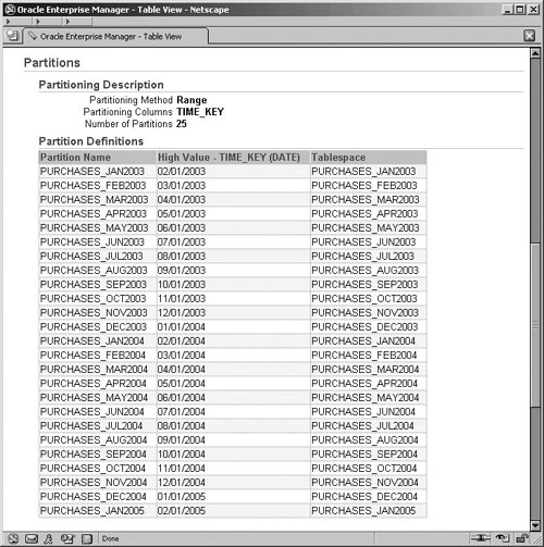
There are a variety of ways to move the data from one table to another in the same database:
Exchange Partition (when the fact table is partitioned)
Direct Path Insert
Create Table as Select
The ALTER TABLE EXCHANGE PARTITION clause is generally the fastest way to move the data of a nonpartitioned table into a partition of a partitioned table. It can be used to move both the data and local indexes from a staging table into a partitioned fact table. The reason it is so fast is because the data is not actually moved; instead, the metadata is updated to reflect the changes.
If the data has not previously been cleansed, it can be validated to ensure it meets the partitioning criteria, or this step can be skipped using the WITHOUT VALIDATION clause. Figure 5.19 shows moving the data from the APR_ORDERS staging table into the PURCHASES fact table using exchange partition.
The following example shows moving the data from the JAN_ORDERS into the PURCHASES_JAN2005 partition of the EASYDW.PURCHASES table.
SQL> ALTER TABLE easydw.purchases
     EXCHANGE PARTITION purchases_jan2005 WITH TABLE jan_orders
     WITHOUT VALIDATION;
Assuming that the PURCHASES_JAN2005 partition was newly created and empty at the start, then, after exchanging the partition, it will be full and there will be no rows left in the JAN_ORDERS table. The JAN_ORDERS table can now be dropped.
SQL> SELECT * FROM jan_orders;

no rows selected

SQL> DROP TABLE jan_orders;
Table dropped.
We discuss table partition operations more extensively in Chapter 11 where we also look at the Enterprise Manager screens to support these operations.
If the fact table is not partitioned, you can add more data to it by using direct path insert. A direct path insert enhances performance during insert operations by formatting and writing data directly into the datafiles without using the buffer cache. This functionality is similar to SQL*Loader direct path mode.
Direct path insert appends the inserted data after existing data in a table; free space within the existing table is not reused when executing direct path operations. Data can be inserted into partitioned or nonpartitioned tables, either in parallel or serially. Direct path insert updates the indexes of the table.
In the EASYDW database, since the purchases table already exists and is partitioned by month, we could use the direct path insert to move the data into the table. Direct path INSERT is executed when you include the APPEND hint and are using the SELECT syntax of the INSERT statement.
SQL> INSERT /*+ APPEND */ INTO easydw.purchases
     SELECT * FROM jan_orders
In our example, the purchases fact table already existed, and new data was added into a separate partition.
Hint
Be sure you have disabled all reference constraints before executing the direct load insert. If you do not, the append hint will be ignored, no warnings will be issued, and a conventional insert will be used. Plus, the insert will take a long time if there is a lot of data. Conventional path is used when using the INSERT...with the VALUES clause even if you use the APPEND hint.
If the detail fact table does not yet exist, you can create a new table selecting a subset of one or more tables using the CREATE TABLE AS SELECT statement. The table creation can be done in parallel. You can also disable logging of redo. In the following example, TEMP_PRODUCTS is the name of the staging table. After performing the transformations and data cleansing, the products table is created by copying the data from the TEMP_PRODUCTS table.
SQL> CREATE TABLE products
     PARALLEL NOLOGGING
     AS
SELECT * FROM temp_products;After the data is loaded, you may need to validate its quality, reenable constraints and triggers, rebuild indexes, update the cost-based optimizer statistics, and refresh the materialized views prior to making the data available to the warehouse users. Some of these tasks have been discussed previously in this chapter.
Run the DBMS_STATS package to update the optimizer statistics on any tables where you have added a significant amount of data. Statistics can be gathered for an index, index partition, table, partition or subpartition, and a materialized view.
Since we added an entire partition to the purchases fact table, the following example will gather statistics for the purchases_jan2005 partition.
SQL> EXECUTE DBMS_STATS.GATHER_TABLE_STATS('easydw','purchases',
'purchases_jan2005',DBMS_STATS.AUTO_SAMPLE_SIZE);If using summary management, run the DBMS_OLAP.VALIDATE_ DIMENSION procedure for each dimension to verify that the hierarchical, attribute, and join relationships are correct. It can also be used to determine if any level columns in a dimension are NULL. You can either verify the newly added rows or all the rows. Any exceptions are logged in the table MVIEW$_EXCEPTIONS, which is created in the user’s schema.
In the following example, the product dimension (parameter 1) in the EASYDW schema (parameter 2) is verified for correctness. All rows will be validated (parameter 3 is set to false), and we’ll check for nulls (parameter 4 is set to true).
SQL> EXECUTE
dbms_olap.validate_dimension('product','easydw',false,true);

SQL> SELECT * FROM mview$_exceptions;

no rows selectedAfter loading the new data into the PURCHASES table, the PRODUCT_SUM materialized view became stale. It only contains information for the existing data and must be refreshed to incorporate the newly loaded data. The operations and options for refreshing materialized views is discussed extensively in Chapter 7.
Next, update the optimizer statistics on any materialized views that may have significantly changed in size. If you used Oracle Enterprise Manager to refresh your materialized views, you have the option of analyzing the materialized view by using the Analyze button on the Materialized View General tab.
To gather optimizer statistics outside of Oracle Enterprise Manager, use the DBMS_STATS package. In this example, table statistics will be gathered from the PRODUCT_SUM materialized view in the EASYDW schema.
SQL> EXECUTE
DBMS_STATS.GATHER_TABLE_STATS('easydw','product_sum'),Back up the database, table or partition after the load is complete, if you used the UNRECOVERABLE option. Since media recovery is disabled for the table being loaded, you will not be able to recover in the event of media failure. Refer to Chapter 12 for a discussion on backup techniques.
Several tools are available on the marketplace to help automate parts of the ETL process, including Oracle Warehouse Builder and tools from Informatica, AbInitio, Ascential, and Sagent. These tools provide the mechanisms to connect to the heterogeneous data sources, generally to either relational databases or flat files, and perform the data extraction functions. They control the transfer of data across a network, provide data transformation services, data cleansing capabilities, and load the data into your data warehouse. We discuss Oracle Warehouse Builder in more detail in Chapter 13.
In this chapter, we looked at the ETL process. Various techniques were discussed to identify rows that changed on the source system as part of the extraction process, and both synchronous and asynchronous forms of Change Data Capture were introduced. A number of types of transformations that are common to a data warehouse were discussed. Examples were shown performing transformations during the load process, using staging tables inside the Oracle database, and using the new regular expression functionality. Techniques used to load the warehouse were illustrated, including SQL*Loader, Data Pump, external tables, and transportable tablespaces. Moving data from the staging system to the warehouse tables can be done using a variety of techniques, such as exchange partition, direct path insert, or create table as select. In Chapter 13, we’ll look at Oracle Warehouse Builder, which uses many of the functions discussed in this chapter, to help you load your data warehouse.
In the next chapter, we will discuss more about how to query the data we have taken so much care in loading.