
So far we have built and managed our database using the SQL*Plus interface or Oracle Enterprise Manager. But there are a number of tools available to the user, DBA, and designer to facilitate easy warehouse creation and access to information. We will now look at three of these tools, which are available from Oracle.
Warehouse Builder
Discoverer
Reports
Oracle Warehouse Builder is a tool that helps the DBA design and manage the data warehouse, whereas Oracle Discoverer and Reports are end-user tools for querying your data warehouse.
Oracle Warehouse Builder (OWB) is Oracle’s tool for designing and deploying data warehouses, data marts, and business intelligence applications. It is part of the Oracle Developer Suite 10g, which includes products for application development, such as Jdeveloper, Designer, and Forms Developer. In the business intelligence (BI) area, it includes the products Oracle Discoverer which is described later in this chapter, Oracle Reports, and Oracle Warehouse Builder.
Building any type of application is not a task to be undertaken lightly; since there are so many steps to be completed when building our data warehouse and BI application, Oracle Warehouse Builder (OWB) is essential. It allows you to:
Design and create the data flows between sources and targets
Design, create, manage, update, and upgrade the data warehouse schema
Manage and update the source definitions
Import data source definitions
Design and create the OLAP and ad hoc query environment
Take advantage of Oracle Database 10g features
Manage the deployment process
Be another repository of the metadata for the warehouse structure, processes, and mappings (i.e., OWB can act as a design tool)
Generate documentation from the metadata
Within OWB there is a repository stored in an Oracle database and this is where OWB keeps all of its metadata. The OWB Client is the main interface and is used to design and create the data warehouse and application.
A code generator is provided that creates the scripts from your design that are applied to the data. The OWB Browser Assistant can be used to view the design and reports from your browser, provided Oracle Application Server 10g has been installed.
You may be wondering why you should use a tool such as Oracle Warehouse Builder to design and create your data warehouse and associated application. Why not design it by hand? Yes, you could do that, but some of the benefits of using Warehouse Builder include:
System design time is reduced, due to the GUI
The design is held in one place, so everyone is guaranteed that he or she is not working with an out-of-date model
The code generated by OWB is free from errors and works the first time
The design can easily be changed or an ETL process modified and then a new module is generated for that change
Let us now look at how we would use OWB to design our data warehouse or data mart.
Before your data warehouse can be designed using Warehouse Builder, a small amount of setup is required to create the repository that Warehouse Builder uses when designing your warehouse. When launching the OWB Repository Assistant, Figure 13.1 appears, which shows us the steps that have to be completed to set up our Warehouse Builder repository. Although there are quite a few steps, this entire process does not take very long, so you will soon be up and running Warehouse Builder.

You can choose into which database the OWB repository will reside, and then you must connect using a user name that has the SYSDBA privilege. Then a user name and password must be supplied for the schema that will own the OWB repository. You must also specify which tablespace to use for repository data and also which language you would like to use. Click on Finish, and your repository is created. Now Oracle Warehouse Builder is ready to use.
Once the Oracle Warehouse Builder repository has been built, it is time to start using this tool to design our data warehouse, where we can:
Define the logical view of our warehouse schema
Define data sources and targets
Describe ETL processes, where we extract, transform and load
Generate the SQL required to create the data warehouse and ETL processes
In OWB, your data warehouse is defined inside a Project, and the following five steps must be completed to build and implement a design:
Create a project.
Define the data sources and targets.
Specify how data moves and its transformations.
Validate and generate the design.
Deploy and run the design.
The OWB client is the primary tool for building our design, and Figure 13.2 shows the console when it is first started.

Creating the project is very straightforward, as this involves simply starting the OWB client, selecting Project from the strip menu at the top, and then selecting Create Project. Give the project a name (our project is called EASYDW), supply an optional description and version number, and the project is created.
The next step is to define where the data for our warehouse will originate. Referring to the OWB Console in Figure 13.2, this could be a database or a file, and a module must now be created that tells us all about that source.
Suppose that one of the sources for our Oracle database comes from our Order entry system, which is in an Oracle database. This source would be defined by right-clicking on Oracle under Databases and selecting Create Oracle Module. Figure 13.3 appears, where the module is named and we specify that it is a data source.

Since we specified that our data source is an Oracle Database, Figure 13.4 appears, where we must specify how to connect to this database. At this time a database link can be created, if one does not already exist, by clicking on the New DB Link button. At this time the link will be tested, so make sure that the database is accessible.
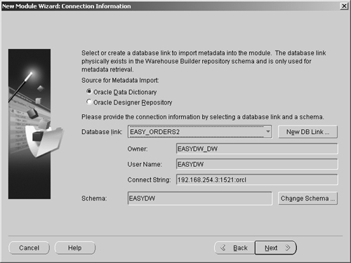
Next, we must specify where this data will be deployed; we have chosen the EASY_DATAW location. By clicking on the Finish button the source and target are now created.
We also have to define the target for our design, which is where the design will be deployed. To achieve this the same process is used as for defining our sources. Therefore, this time in Figure 13.3, we would specify THE_EASYDW_DW, which is the name we want to give to our design, and click the radio button for Warehouse Target.
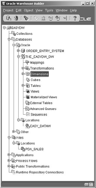
If there are any file data sources that will be input to our data warehouse, these can also be defined at this stage. Suppose that customers can also place orders via PDA devices. These orders are captured from the device and are currently stored in a file for subsequent processing into the system. This data source can be defined by right-clicking on Files in Figure 13.5 and then selecting Create Flat File Module. The details of this flat file are entered into the wizard, and the data source, PDA_SALES, has now been defined.
This process is repeated for every data source in our system, and OWB provides for several standard data sources, including, flat files, SAP, Oracle database, or other databases such as DB2.
After doing all of this work, it is extremely important to save it, because OWB does not automatically save your work. Therefore, whenever you are satisfied with the state of the objects, you must Commit the changes by either clicking on the commit icon or selecting Commit from the Project option on the strip menu at the top.
In the previous section, we defined the sources for our data and our data warehouse. Now is the time to define the tables that we require inside our data warehouse. This can be achieved by either defining the tables manually or importing them from another database.
Importing the table definitions illustrates how OWB can save on development time, because it can be quite time consuming and error prone defining the tables by hand. When you are defining these tables, which are going to be the sources for your data, its very important that they are defined exactly as they exist in your production system; otherwise, costly delays will incur when trying to resolve the data inconsistencies. If you have to define them by hand, then it’s easy to make mistakes, which can subsequently delay implementation of your data warehouse.
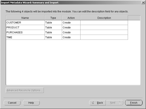
The table definitions are imported by right-clicking on Database and selecting Import. The Import Metadata Wizard will appear for you to answer the questions as to what is to be imported—tables, sequences, and so on. Upon completion, Figure 13.6 appears, where we can see the tables that have been imported from another database.
Some of the tables may have to be defined manually, and this can be achieved by double-clicking on THE_EASYDW_DW database source shown in Figure 13.5, then right-clicking on Tables, and then selecting Create Table. This will start the new table wizard; Figure 13.7 illustrates how the columns are specified. Here we have defined a new table called COUNTRY.

While using this wizard don’t forget that you can also specify constraints, such as primary-key, foreign-key, and check constraints. When the definition is complete, click on the Finish button to complete the definition of our table.
Typically, a data warehouse consists of tables, which can be fact and dimension tables; in the previous section, we saw how to physically create tables. At this stage in the development of our data warehouse, we probably only have a model, described in terms of facts and dimensions. OWB allows us to define these logical objects and then, when it is time to generate our design, OWB will physically create the tables to represent these facts and dimension.
A dimension is created in OWB by using the dimension wizard, which is selected by right-clicking on the Dimension object, shown in Figure 13.5, and selecting Create Dimension.
The process is very similar to the one we saw in Chapter 8 for creating a dimension. That is, you must name the dimension, define each level and its attributes, and then describe the hierarchy. In Figure 13.8, we see one of the dimension wizard screens where we are defining the hierarchy for our customer dimension.

Once the dimensions have been created, the next step in our design process is to define one or more fact tables, which are known as cubes. In OWB a cube is a logical object in that only when the physical design is generated, does our cube become a physical table. It is created by right-clicking on Cube in Figure 13.5 and selecting Create Cube; the New Cube Wizard appears. One of the screens is shown in Figure 13.9, which is where the foreign keys for our cube are defined. In this example, OWB automatically offers a foreign key to each dimension that was previously defined.
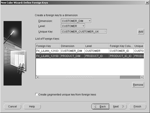
The wizard also allows you to add measures and by clicking on the Finish button our cube is created.
At any time while the data warehouse is being defined, the various parts of the design can be validated by selecting the Validate option, described in section 13.2.8. Any problems, can be correctly immediately before proceeding to defining the next part of the design.
There are a number of other objects that can be defined but will not be described in this chapter. They include materialized views, external tables, sequences, and views.
In Chapter 5, we saw that when data is being moved from one source to another, it often needs to undergo some transformations. In OWB we can define these transformations using functions, procedures, and packages.
The real power of Oracle Warehouse Builder starts to become apparent when we see how it can be used to define how data is moved from our sources, such as from our OLTP system into our data warehouse. In Chapter 5, we discussed the various techniques that we can use to load and perform transformations. Now, inside Oracle Warehouse Builder, by using its GUI interface, we can graphically represent these processes by defining a mapping. When the design is finally generated, OWB even creates the procedures required to transform and load the data, using the principles described in Chapter 5. Now we will look at just a few of the many different types of mappings that are possible.
A mapping is defined from the OWB client by right-clicking on Mappings, in Figure 13.5; selecting Creating Mappings gives the mapping a name and then the Mapping Editor appears, as shown in Figure 13.10. The first mapping that we are going to define is extracting information from our ORDER_ENTRY_SYSTEM and moving it into our data warehouse. OWB can also take information from flat files or from SAP, but we won’t be showing here how that is done.
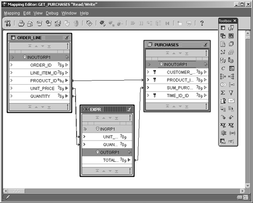
When the blank Mapping Editor appears, click on the Mapping Table icon (which is top left in the floating toolbar) and drag it onto the Editor. It now asks you where your table is to come from, and we are going to select the ORDER_LINE table from our source ORDER_ENTRY_SYSTEM, which we defined earlier. Then click on the Mapping Cube icon and select PURCHASES. Now in our Editor we have two tables: ORDER_LINE and PURCHASES.
The next step is to specify which items are to be moved from each table. First, we are going to move the item PRODUCT_ID from the ORDER_LINE table to the PURCHASES table. This is achieved by dragging a line from PRODUCT_ID in ORDER_LINE to PRODUCT_ID in PURCHASES. In Figure 13.10, we can see the line that OWB has drawn between the two items.
The next column to be defined in PURCHASES is the value of the order, and this can only be obtained by computing its value from two columns in the ORDER_ITEM table. To compute this value an intermediate expression box must be created, as illustrated in Figure 13.10.
Click on the Expression icon and drag that onto the Mapping Editor. An empty box appears with empty input and output groups. Take the two columns from ORDER_LINE, unit_price and quantity, and drag them over to the input group box. Now we have to use the right mouse button to add a new attribute in our output group, which we will call Total_Price. Do this by choosing Edit from the right mouse menu, and under the Output Attribute tab add the new attribute, called Total Price.
Then you select that item’s properties and click on the expression box and the expression builder will appear, where you can specify how the attribute is to be computed, which in our case is to multiply the two numbers together. Then drag a line from TOTAL_PRICE to the column SUM_PURCHASES in PURCHASES to complete the mapping operation.
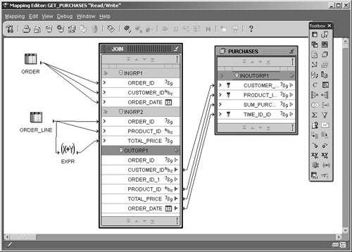
Another common task that our warehouse designer has to perform is joining data from two or more tables to extract information that is used as input to another table. In Figure 13.11, we see a join that we have created between ORDER and ORDER_LINE to enable us to store one record in our data warehouse for the total value of the order. Note that the expression that we created in Figure 13.10 has now been used as input to the join.
Previously in this book we have described surrogate keys, where the natural keys used in the sources for your data warehouse are transformed into a key used by the data warehouse. In OWB we can define exactly how that transformation should occur by using the key lookup feature.
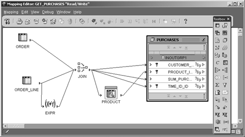
In Chapter 5, we described the process of converting the product code used in out OLTP system to a surrogate key in the data warehouse. In Figure 13.12, this has been implemented in OWB by showing that the column PRODUCT_ID from the join between ORDER and ORDER_LINE is input to the key lookup process. Although not visible, a mapping has been defined that states that PRODUCT_ID is to be matched to PRODUCT_ CD. The resulting output is the column PRODUCT_ID, which is sent to the PURCHASES table.
When data is being extracted from sources such as our OLTP system, there may be times when we do not want all of that data to be sent across to our data warehouse. In OWB, this is not a problem, because it allows us to filter the incoming data in a variety of ways.
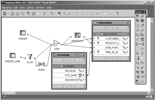
In Figure 13.13, we are filtering the items from the ORDER_LINE table according to criteria that we have specified. For example, we could say that we are only interested in certain products. Also see in our example how, after we have filtered the data, we are then applying the expression we defined in Figure 13.10 to the data that has passed through the filter.
There may be times when, rather than extracting data from a source, the data must be automatically generated. OWB has this capability, and it can automatically create:
Record number
Sequence number
System date
In Figure 13.13, we can see the system date being used to set the date for our order. This was achieved by dragging the Data Generator icon onto the Mapping Editor, and then selecting the item required and attaching it to PURCHASES.
Over these few pages, we have barely touched the surface on the types of transformations and mappings that are possible with Oracle Warehouse Builder. All of the icons shown in the toolbox in Figure 13.13 can be used to define your warehouse. Also, in these examples we have kept them simple, but in a real warehouse, they would be connected; we did start to show this in Figures 13.12 and 13.13 where the expression was being used as input to another stage in the loading process.
Once the design is complete, or while it is being developed, it must be validated before Oracle Warehouse Builder can create all the components needed to build, load, and manage our data warehouse. You can validate each component individually, or the entire project, but it’s probably easier to resolve problems if you validate each component as it is defined.
To validate any component, select Object from the strip menu at the top and then select Validate, or it can be selected by clicking on the right mouse button. In Figure 13.14, we can see that there are several errors with our design. We can’t use SYS_DATE for the time in the purchases column and, more importantly, OWB has detected that the data types of the CUSTOMER_ID column are incompatible between the ORDERS system and the data warehouse. Therefore, we need to fix these problems before we can continue.
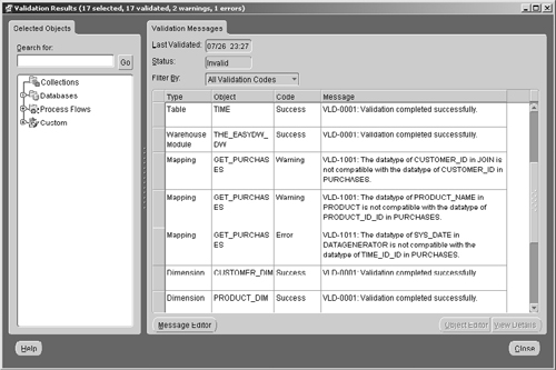
This illustrates the benefits of using a tool such as OWB, because with a complex design it is very easy to miss a problem such as the one in Figure 13.14 until very late in the day. We have known of systems where data type inconsistencies were only detected the first day someone tried to transfer data from the source system.
Once the design has been validated, Oracle Warehouse Builder can now generate the design. From the OWB client, shown in Figure 13.5, we can generate each component individually or by selecting Generate. The generation process will run and OWB will create scripts that perform the following tasks:
SQL for creating the database
PL/SQL for executing within the database
Procedures for loading the data
SQL*Loader files for working with our flat files

In Figure 13.15, we can see the various components that OWB will generate. There are the schema objects, such as our PRODUCT table. By clicking anywhere on the PRODUCT line, everything that OWB created for the PRODUCT table is displayed in the lower part of the screen.
By clicking on the Validation tab, the validation messages are shown, and clicking on the Script tab lists all the scripts created for this object. To view the script, click on the script name and then click on View Code.
If we click on the Mappings tab, we would see that OWB has created a package for us to load the data, which we defined previously. By clicking on the View Code button, we can see part of this long procedure generated by OWB (Figure 13.16). Just look at where the slider bar is to see how much code OWB has created for us. The section of code we have shown here is part of the INSERT statement, but prior to this there are variable definitions and lots of other things that we would have had to write ourselves.
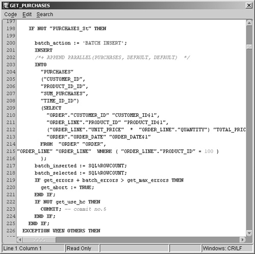
In this example, OWB has chosen to use a SQL INSERT statement, but since OWB has been designed to take advantage of features in the database, it can therefore use statements such as MERGE, which we saw earlier in the code that it generates.
Vast amounts of time can be saved using OWB, because you no longer have to write the code needed to implement and load data into your warehouse. The code that OWB generates is optimized for the Oracle database and it works immediately. When was the last time you wrote a complex piece of code that worked the first time?
Now the time has come to implement our design, but before this can be completed, you must ensure that the runtime repository has been created on the system where your design will be deployed, because this is where all the information about your deployed system is stored. This task should have been completed when OWB was installed, but it can be performed at any time by running the OWB Runtime Assistant.
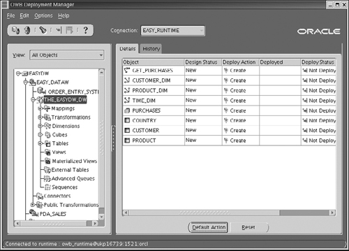
Launch the Deployment Manager from the OWB client by selecting File from the strip menu at the top and Figure 13.17 appears. Here we can see all the objects for our system, such as the PRODUCT table and the CUSTOMER_DIM dimension. To deploy an object, click in the Deploy Action box to specify the action required, which, in Figure 13.17, is create.
Once all appropriate actions have been set for the objects, to actually deploy them, click on File in the strip menu at the top and then select Generate/Deploy. A status bar will appear showing how deployment is progressing.
The next screen to appear is that shown in Figure 13.18, which is the predeployment report, where we can see the state of every object. Referring to TIME, it has completed validation, and by clicking on the Script tab, we can see all the scripts that will be generated.

Select the script, and then click on the View Code button to view the contents of any of those scripts. When you are satisfied with what is to be built, click on the Deploy button and your system will be generated.
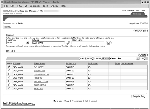
The design has now been generated, and in Figure 13.19, which is a screen from Enterprise Manager, we can see the all the objects created by the deploy operation in our new schema, EASY_OWB.
Returning to the Deployment Manager, we see that in Figure 13.20 that the status of all of our objects is displayed and that everything was successful except for the GET_PURCHASES mapping. OWB did tell us about this problem earlier, but we decided to deploy regardless, because it was not affecting the deployment of any other objects.
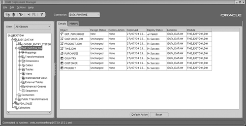
With virtually all of the system deployed, OWB allows us to go back to the OWB client, fix the problem with the GET_PURCHASES mapping, and then repeat the deploy process; however, this time it would only be performed on this object.
Although we have generated a logical design, it is most likely that it does not include all of the physical aspects of our design, such as whether a table is partitioned and which indexes are needed. These physical components can be configured in OWB by selecting the module to be configured, right-clicking on the mouse, and selecting Configure. Figure 13.21 is displayed, which lists all of the properties that you can configure. In this example, for our COUNTRY table, we can see that an index has been defined, and the table is going to be stored in tablespace USERS.
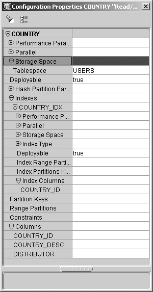
When defining indexes, OWB has the ability to automatically recommend bitmapped indexes; clicking on the Generate button shows these recommendations.
Normally, the physical design for the objects would be done prior to deployment. However, in our example we have created the EASYDW warehouse and then returned to OWB, defined more physical design attributes, and then redeployed.
Hopefully, you now have an appreciation of what OWB can do. This is a very powerful product and, over these few pages, we have only been able to highlight some of its features. What we have not covered here is how OWB can be managed using a browser and integrated into Oracle Portal.
There are many benefits from using tools such as Oracle Warehouse Builder. It provides a visual representation of your warehouse and, by using the various wizards that are available, it is easy to complete the tasks needed for building the warehouse. In addition when changes to the environment occur, you can visually see the impact of them and OWB can easily incorporate them into the environment. The Deployment Manager enables you to clearly see the state of all modules in the system and view the code for those modules.
Now that you have deployed the physical design to the database, you may want to enable this for a query tool. OWB has the capability of transferring the design metadata into a Discoverer environment, which is described in the next section. By doing this you can save yourself time and effort in creating the reporting solution on top of your logical design. A second benefit is the concentration of metadata in a single place, allowing you to reduce the maintenance efforts for your integrated solution.
Oracle Warehouse Builder provides a comprehensive environment for building and managing your data warehouse that could significantly reduce your development time and costs when its full potential is exploited.
Oracle Discoverer is an extremely popular tool for querying data warehouses and generating reports, because it is very easy and intuitive to use and has been designed for use by end users who are focused on the business aspects and not necessarily familiar with databases. Therefore, in order for these business users to be able to use Discoverer easily, some setup is required from the DBA group. But once this has been done, these end users should really like using this tool. There are four parts to Oracle Discoverer:
Administrator
Desktop
Plus
Viewer
Discoverer Administrator is the version that is used by the power user or analyst of the data warehouse to set up the environment for the general Discoverer users. The business end user will either use the Desktop or Plus version, because it has been designed especially for people who are not familiar with writing computer programs, as well as for anyone who is not familiar with SQL and prefers to deal with data using familiar business entities. For business users and others who may be concerned that they could change the data within the data warehouse, fear not, because Discoverer Viewer allows the user to only view predefined reports. The attraction of using Discoverer Viewer is that all users require to access the data is their PC and a browser.
Oracle Discoverer is also integrated with Oracle Portal, which we will learn more about later. From within Oracle Portal it is possible to set up Web pages that have direct access to Discoverer reports on our data, thus providing a very powerful and dynamic mechanism for displaying information.
Oracle Discoverer is part of Oracle Application Server and it can be run in one of two ways. When Oracle Developer Suite is installed, this provides access to Discoverer Administrator and Discoverer Desktop, which are the original, nonbrowser-based versions of Discoverer. Currently, Discoverer can only be configured using the Discoverer Administrator therefore, Oracle Developer Suite will have to be installed.
Discoverer requires some configuration, which will be described shortly, before it can be used by general users. Once this task is complete, it can then be queried using Discoverer Desktop; however, you may prefer to use one of the browser-based tools, Discoverer Viewer or Plus, due to the additional capabilities these offer because they are tightly integrated into Oracle Application Server. Some additional setup and configuration is required when Discoverer Viewer and Plus are used, but it is worth all the extra effort.
Oracle Discoverer can also be used to access data held in non-Oracle databases, using Oracle Heterogeneous Services. A single business area can be created that references data from these different data sources. Then, Discoverer functionality, such as report scheduling, query prediction, and use of analytical functions, can be used against this non-Oracle data.
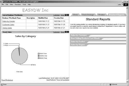
Before we learn how to set up Discoverer, let’s first look at the types of reports that it can produce. Imagine logging on to the corporate Web site and having available to you reports containing the latest data from Discoverer, along with other company information. Figure 13.22 illustrates its capabilities with Oracle Portal, where we can see a list of all of the reports available to us in its only region on the screen. In another region, one of the reports is displaying its results in a pie chart. Since each user of the Portal can have his or her own customized view, it can greatly improve productivity and business efficiency.
Many organizations run Discoverer independently, and Discoverer Viewer provides a user with the ability to access predefined reports and have the capability to modify those reports in a limited way. The advantage of this approach is that the user only needs a PC and a browser to access the data in the warehouse and the DBA can rest assured that users cannot change the data.
You can start Discoverer viewer from your browser using a URL such as:
http://easydw.com:7777/discoverer/viewer
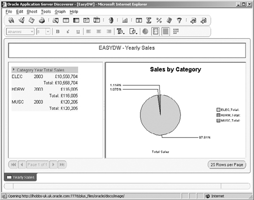
A connection is made to this database, and a list of the available workbooks that we can attach to is presented. We select our workbook, EASYDW and the query contained within is immediately executed. In Figure 13.23, we can monitor the progress of our executing query, and when it has completed our report is displayed, as shown in Figure 13.24.
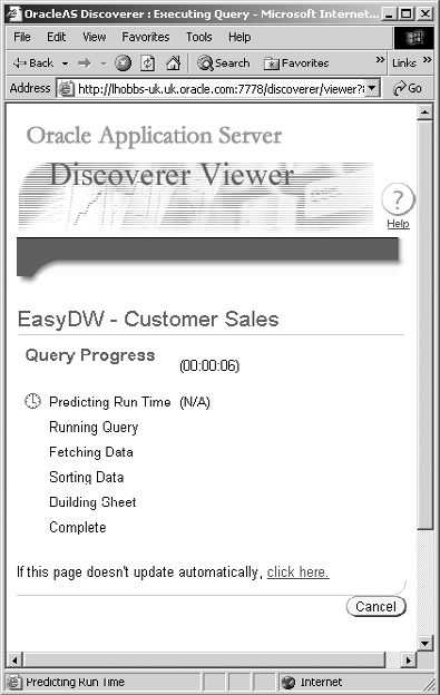
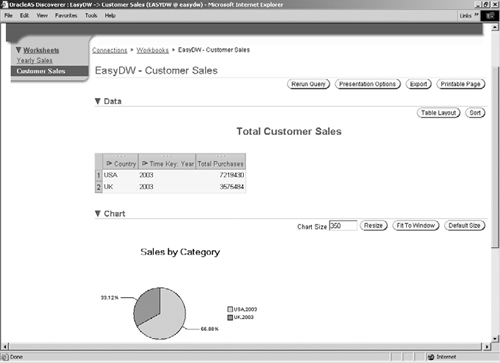
Since we defined this report as both a table and a graph, both versions are displayed in Figure 13.24. Note that at any time we can hide the graph or table by clicking on the Data or Chart option. The report shown here is the default generated by Discoverer, and I am sure you will agree that it is a very nice format, which is presented well and is easy to understand.
Inside a workbook there can be many reports. In Figure 13.24, we can see a list of those reports in the top left. Any of these reports can be run by simply clicking on the report name.
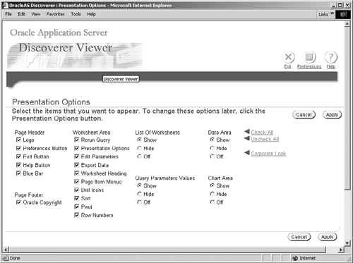
One of the advantages of using Discoverer Viewer is that is the user is not able to change the data in the warehouse or generate new reports. However, there are limited customizations that can be done to this report, such as changing the sort order or table layout, or, by clicking on the Presentation Options items, as illustrated in Figure 13.25, changing how our report looks.
One of the features that makes Discoverer nice to use is the ability to group together a number of reports that can be easily run and customized to your own requirements. In the example shown here, we have a workbook called EASYDW and, referring to Figure 13.24, at the top left of the screen we can see a tab, with two entries on it, for each of the reports that are available:
Yearly Sales
Customer Sales
In Figure 13.24, we see both a table and a graph generated from data in our warehouse. When this report is run, the user is prompted to specify his or her criteria for which years the sales are to be displayed.
When a report is produced, someone reading it may say that this is very interesting, but I need to know more about how this data is derived. For example, suppose the user is viewing the report shown in Figure 13.24 and sees that we sold many items in the United States, but how does that break down by state and is it more than we sold in the United Kingdom?
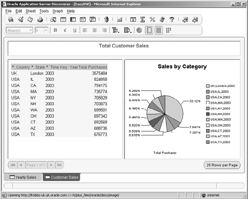
By clicking on Country, a drill-down list is displayed and State was selected; Figure 13.26 shows us the report with the data by state. Now we can see that we sold across a number of states, rather than in just one state, and U.K. sales are equivalent to selling in over four U.S. states.
Now that we have caught a glimpse of the types of reports, Discoverer can produce, we must return to setting up Discoverer, because, before you can use it, that setup we mentioned earlier must be performed.
When a database is created, usually everything is named using terminology that is familiar to a computer-literate person, but for a typical end user it may look like a foreign language. Oracle Discoverer overcomes this problem by creating what is known as the End-User Layer. Here, all those technical computer terms are turned into a user-friendly environment so that it is easy for anyone to understand and access the information in the database. Therefore, this task has to be completed before anyone can access the database. This may seem like a lot of work, but, once completed, it will make it very easy for users to access all the information, thus saving countless phone calls to the IT department.
A major advantage of this approach is that it enables an organization to control exactly which data in the warehouse users can see how they see it, and, most importantly, they won’t need to understand how to join data in order to query the data warehouse. To begin using Discoverer, first connect to your Oracle database.
Hint
You may prefer to create a special user for Discoverer and connect to your database using that user to ensure that the metadata is loaded under that user name.
The first time the Discoverer Administrator is started, you will be asked to create an end-user layer (EUL), which consists of all the metadata that is needed by Discoverer; therefore, this task will be performed only once. Figure 13.27 shows the screen where you can manage the end-user layer, including creating a new one or deleting an existing one.
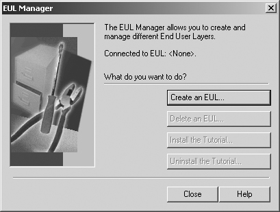
The wizard will then ask who will own the EUL. In our example, it would be EASYDW. Now click on the Finish button and the end-user layer is created. This process may take a few minutes, depending on the complexity of the schema that it has to analyze.
Once the definition of the end-user layer is complete, a Business Area is named, where all of the information needed to query the warehouse must be defined. The purpose of the business area is to group information into business-oriented categories, such as Sales or Finance, which are familiar to end users. Business areas are the unit of access control and a user can be assigned to one or more business areas. Users will then have access to all of the objects within the assigned business area.
Within this business area, you will specify exactly which data a user may access, how that data may be joined, and describe data aggregations and new data items based on calculations on existing data items. Creating the business area will take some time, but it will reap significant benefits later.
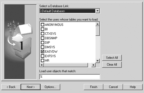
When creating the business area, we must first specify the schemas from where data is to be made available to the end user, as illustrated in Figure 13.28. We can select any number of users from the list and also request that it only selects items from the list that match the pattern specified in the box. In our example, we have selected only the user, or schema EASYDW.
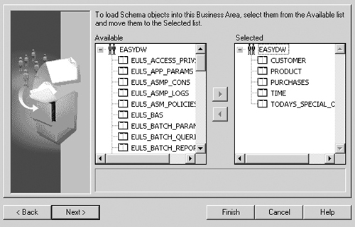
Once we know the schema from which the data will be available, we can then explicitly state from which tables or views we can retrieve data, as shown in Figure 13.29. Using our Easy Shopping Inc. example, we have given the users access to all of the five tables in this data warehouse.
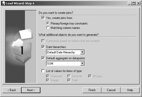
One extremely useful feature in Discoverer is the ability of the wizard to automatically create joins based on primary and foreign keys and create hierarchies from the data, as illustrated in Figure 13.30. By allowing the wizard to perform these tasks, there will be less setup work for you to do, and by default these options are already selected. The advantage to the end users is that when they are constructing queries they won’t need to know how to join the data, because Discoverer will know this from what was done at this stage. Therefore, end users require minimal computer design knowledge in order to construct reports in the database.
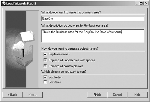
There is one final screen before the first stage in creating the business area is complete. In Figure 13.31, we must name the EUL and optionally add a description to describe what is being held. Discoverer will also generate names for all of the objects, and in Figure 13.31 you can see the options available, such as capitalize or replace underscores with spaces.
Clicking on the Finish button, completes the first stage in creating our business area. A task list will appear, as shown in Figure 13.32, to help remind us of the steps to follow.

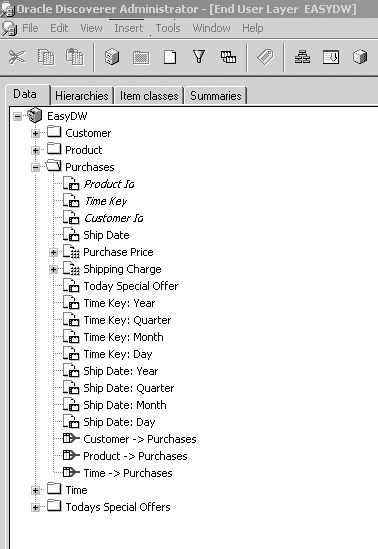
In Figure 13.33, we can see that part of the basic EUL screen in Discoverer from where everything can be managed. Discoverer has already identified that the table PURCHASES can be joined to the customer, product, and time table and that some computation may be applied to the column purchase price.
With the basic EUL is place, this is where the real work begins, since we can now set up the rest of the business area; although we have shown only the creation of one business area, you could create any number of business areas in your environment, each with its own unique set of data requirements.
By default, when access is given to a table, all the columns in that table are accessible. What is nice about Discoverer is that users can only access data via the business area. If the table and column are not given visibility by Discoverer, then the user will never even know that this data existed.
In Figure 13.33, we can see all the tables from the database that we have access to. Note that our table TODAYS_SPECIAL_OFFERS is now called Todays Special Offer, as a result of the naming change requested earlier. By default, the end user will have access to every column in those tables. If you click on the table name to expand it, all the columns in that table will appear. To remove any of those columns, simply click on the item using the right mouse button, and a drop-down list will appear. One of the items in that list is Delete Item. Simply select that option, and the item will be removed from the business area but not from the database.
Before moving on, there is some terminology that you should familiarize yourself with. In Discoverer, a table or view is known as a folder, and a column from the table is called an item. A folder can be one of two types:
Simple, where it is based on a single database table or view
Complex, where it can contain items from other folders and can be nested
An item corresponds to a column in a relational database. A simple item is based on a single column in the database, but an item can also be calculated or derived based on a formula using other items, functions, or operators.
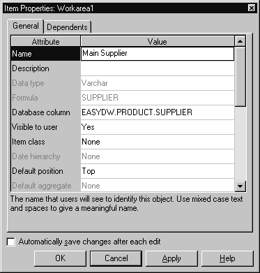
The attributes of any of the items that you have selected may be modified by selecting that item, clicking on the right mouse button, and then selecting Properties. The window illustrated in Figure 13.34 will appear, and you can then modify whichever properties you like. In this example, we have changed the item’s name from Supplier to Main Supplier, which means that our users can be presented with friendly meaningful names, rather than computer format names.
When the business area is first created, if the database has primary and foreign keys defined, then Discoverer will automatically create joins between those constraints. However, you can specify your own joins by selecting Insert from the strip menu and then Joins.
Another feature that many DBA’s may require is the ability to create new columns or items in the database by calculating their results from other columns.
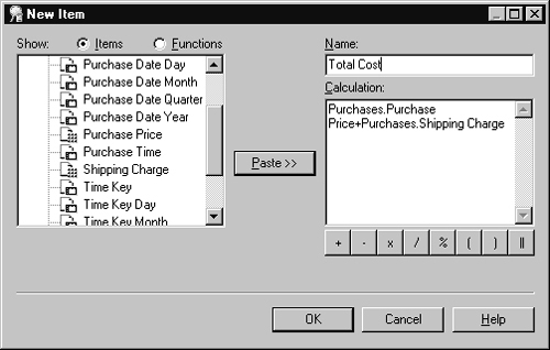
A calculation creates a new item in the end-user layer. It will not add underlying columns to database tables and is used to create a new item where there is no underlying database column that contains the data required. Calculations can be simple, such as weight * 4.54 or they can be complex mathematical or statistical expressions. For example, in Figure 13.35, a new column called Total Cost is created in the PURCHASES table by adding together the columns purchase price and shipping charges. You can create as many of these types of calculations as you require, and they will appear as an item for that table.
When the EUL was first created, Discoverer tried to identify which joins to create from the primary- and foreign-key relationships that had already been defined. However, there may be times when additional joins are required and these can easily be created using the join wizard.
A join is created by clicking on Create Joins in the Discoverer Administrative Task List, which is shown in Figure 13.32, or from the Administration Work Area, shown in Figure 13.34, by clicking on Insert and then Joins; the wizard will then appear, as illustrated in Figure 13.36.

By using the wizard, give the join a name and then, from the drop-down list, select the table and columns to join on and the type of join. In our example in Figure 13.36, we have specified a join between the TODAYS SPECIAL OFFERS table and the PRODUCT table using the column PRODUCT_ID. The advantage of defining these joins now is that when a user writes a query, Discoverer will know how to join the data, so it’s one less piece of information that our user has to supply; in this way we ensure that a meaningful join is being applied.
Click on the Next button to proceed to the second and final join wizard screen, where you can specify some more advanced options about the joins.
We have already seen that hierarchies play an important role in our data warehouse. Although in Oracle we can create dimensions, at the time of writing, these are not used by Discoverer, and we must create our own dimensions, which are known in Discoverer as hierarchies. Hierarchies are very important in Discoverer, because if an item is in a hierarchy, then users can:
Drill up, which changes the query to show a higher level of details
Drill down, which shows more detail
This is how we were able to drill on our report shown earlier. A hierarchy is created by clicking on Insert in the menu at the top and then selecting Hierarchy. First, you will be asked about the type of hierarchy you want to create: an item or a date. When the business area is first created, it is quite likely that Discoverer will automatically create a time-based hierarchy. Therefore, you will probably only have to create nontime-based hierarchies.
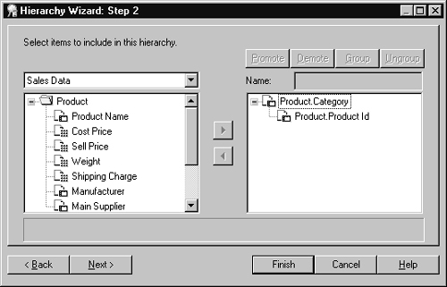
Figure 13.37 shows how easy it is to create the hierarchy by selecting the items and then defining the hierarchy relationship. In Figure 13.37, we have created a very simple hierarchy between PRODUCT_ID and CATEGORY.
Hint
Click on the Hierarchy tab shown in Figure 13.34 to see all the hierarchies that Discoverer created automatically when the EUL was generated.
When the end users are actually querying the data, there are times when it may be helpful to them if they can see a possible list of values. For example, suppose they want to pick out all of the electrical items. If they know which category they are represented in, then this will facilitate rapid query generation.
An item class can describe the hierarchical relationship between items, a list of values, alternative sort keys for items, and the display methods. Therefore, an item class defines all of the attributes for an item. Once an item class has been defined, it can then be assigned to other items, which share similar properties.
An item class is created by selecting Insert from the menu at the top and then Insert Class from the list or by clicking on the text in the Administration Task List, shown in Figure 13.32, the Item Class Wizard will now appear.
The first step is to define the type of item class, a List of Values, Alternative Sort, or Drill to Details, which is used to drill between a summary and the detail. Then all you have to select is the column containing the values and which tables will use it. When it is complete, click on the tab Item Classes, and the window shown in Figure 13.38 will appear.

In this example, a list of values called Categories has been created from our products dimension table. If we expand the entry categories, the data warehouse can be queried, and all the different values will be displayed; in Figure 13.38, we can see some of the different categories for products that are sold. Here we only have a few items, but in the real world, where you may have a number of different values, you can omit this step of displaying the results.
When an item class is defined, you can also define the sort order for the data. In Figure 13.39, we have chosen to use the conventional alphabetical method, but that is not always suitable, so Discoverer will allow you explicitly to specify a logical order, such as N, S, E, W (North, South, East, West) rather than E, N, S, W.

We have already seen the importance of creating and using materialized views in our data warehouse in Chapter 7. Discoverer allows you to create your materialized views, which Discoverer calls summaries, from its summary wizard, by:
Using query performance statistics
Manually creating the summary
Registering a previously built summary
To create your summary, click on Insert in the menu at the top, and then select Summary and the summary wizard appears. Three types of summaries can be created:
Specifying items in the end-user layer
Recommendations based on query performance statistics
Registering an existing summary table
Then the window shown in Figure 13.39 appears, where you select the folders and items from within those tables that are to appear in the summary. In our example, we have selected only the PURCHASES table, but you could select multiple tables. Then we have chosen four of the data items in that table. For the item purchase price, we have asked that this value be aggregated. You will see that Discoverer will automatically supply a range of functions for you to select when a function may be applied to an item. In Figure 13.39, for the item PURCHASE_PRICE, we have asked that the SUM function be applied to this item. Next, you are asked to specify which groups of items you require.
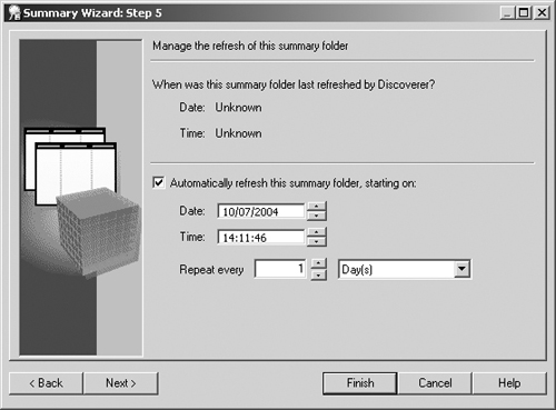
As we have seen, it is very important to ensure that the materialized views or summary contain the latest data. When defining your summary in Discoverer, you can specify how often it is to be refreshed. Remember that, as new data is added to the warehouse, the summaries must be maintained to reflect the latest data. In Figure 13.40, we can see that we have stated that this summary should be refreshed every day.
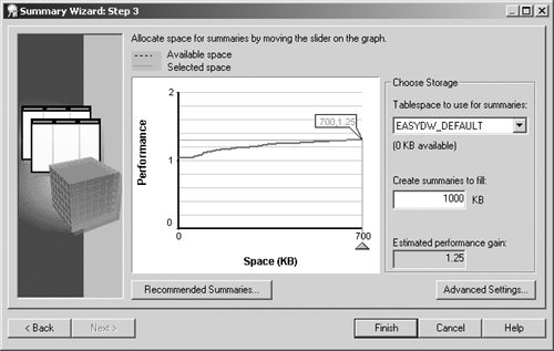
If you don’t know which summaries to create, Discoverer can recommend them for you using its own summary wizard. In Figure 13.41, we can see one of the steps from the wizard, where we can select the summaries we require based on our space requirements. This wizard is very similar to summary management’s own SQL Access Advisor, described in Chapter 10, but the recommendation process used by Discoverer is different from the one used by the Oracle SQL Access Advisor.
Creating either Discoverer summaries or materialized views is very important if you want to achieve the fastest query response time. Here, we have seen how to create summaries directly in Discoverer, but you can create materialized views, as discussed in Chapter 7, or use the SQL Access Advisor, which was described in Chapter 10. Irrespective of how the materialized view is created, Discoverer will still use it whenever possible.
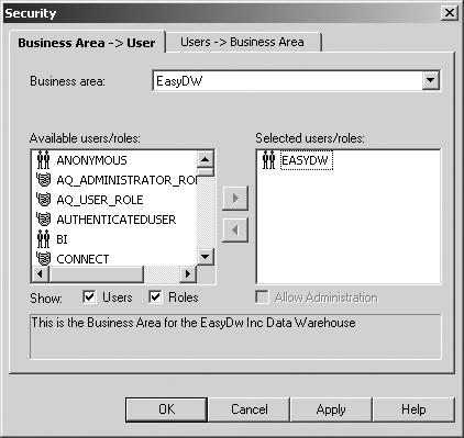
The final setup task is defining who may access the business area that you have just created. You can start this component by double-clicking on Grant Business Area Access, shown in Figure 13.42. A window will appear that will allow you to state which users can access a business area or which business areas a user can access. In Figure 13.42, we can see that the only user who will be granted access to our business area is EASYDW. Don’t forget that although in this example we have enabled access via the user name, you can also grant access to the business area via the roles that may be given to a user. When you are satisfied that all the relevant access rights have been given, click on the Apply button to complete the changes.
In Figure 13.43, our complete business area is shown. Expanding just the PURCHASES table, we can see all the items that are available to our users; the new calculation that we created, called Total Cost; and the functions that we can apply to that column. At the bottom of the window, we can see that joins have been created from the PURCHASES table to the PRODUCT and TIME table. Of course, not all the information can be displayed on this one window, so, to see the Hierarchies tab, you will have to click that tab. The same is true for item classes and summary information.

We have now completed all of the basic setup tasks for using Discoverer. Don’t forget to save all of your work, and please remember that the tool is much more comprehensive than we have shown in these few pages. For example, we haven’t shown here that Discoverer fully supports the Oracle analytical functions to enable sophisticated analysis of the data. Now we can start using Discoverer Desktop, Viewer, or Discoverer Plus to retrieve data from our data warehouse.
Once the environment has been set up for querying via Discoverer, you can now start either the Desktop edition or the Plus version, which has been designed for use via a browser. In this chapter, our examples will use the browser version, Discoverer Plus.
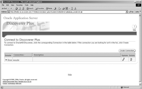
Reports in Discoverer are held in a workbook; therefore, the first step is to connect to the database where our workbooks reside. In Discoverer Plus, launch Plus from your browser using a URL such as:
http://easydw.com:7777/discoverer/plus
You will be presented with a list of the databases that you can connect to, as shown in Figure 13.44. Here we can see that we only have one database, called EASYDW.
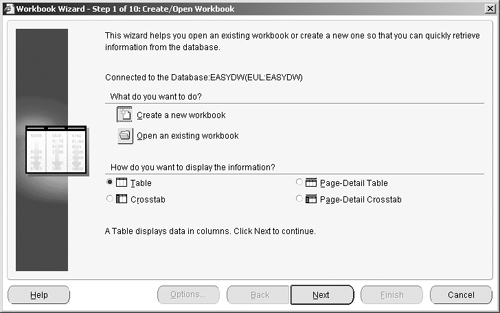
These connections will have been defined previously and consist of your user name and database name. Therefore, all you must supply is your password, and you will be asked whether to create or open an existing workbook. In Figure 13.45, we see the initial window, where we specify the workbook and how the results are to be displayed. Discoverer offers a range of display options, such as showing the data in tabular or a crosstab form. Using the crosstab format is ideal when you have multidimensional data to display.
Now, it is time to specify exactly what is to be reported in this query. First, you must select the business area that was defined using the Administration edition, which determines the data that you may see. In our example, we have only the EASYDW business area, but there could be several areas to choose from.
Now we have to select the items from those folders. This is a simple process, involving moving them from the left window (available) to the right window (selected). In Figure 13.46, we have selected the item category from the product folder, purchase price from the purchases folder, and the year from the time folder.

Next, we must specify the layout for our report. This is very easily achieved by dragging the columns to where you require them on the report. In Figure 13.47, we have specified our order as category, year, and price. Initially the year column was to the right of the purchase price column, but by simply dragging the year column, we can place it wherever we wish on the report. At this stage, we can only decide how the data is to be presented; we can specify formats and headings on another screen.

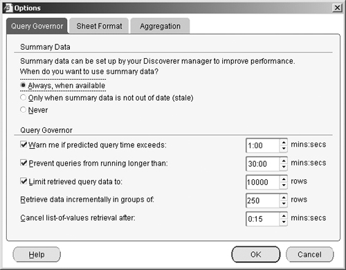
At this stage, by clicking on the Options button, Figure 13.48 will appear, and, in Discoverer, some very useful limits can be set on the query, such as preventing it from running longer than a specified period of time or only returning a limited number of rows.
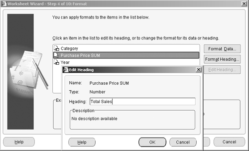
For each item that will be displayed on our report, we can now specify how that data is to be formatted and the heading to be used on reports. In Figure 13.49, we have changed the heading for our sum on PURCHASE_ PRICE to Total Sales. By clicking on the Format Heading button, the font and alignment options can be defined, and clicking on Format Data allows us to specify how the data is actually presented. In this example, we have decided that our total will have no decimal places.
Progressing through all of the steps in the wizard shows a number of other options that are available, but we will not show all of these steps here. For example, a condition can be specified to limit the results of our worksheet to a specific criterion. There are some very extensive options available here, however, in this example we are going to view all of the data.
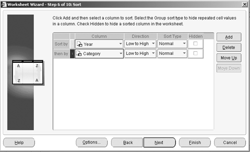
Step 6 in the wizard is specifying the sort order of our data, which is achieved by clicking on the Add button and selecting one of the available columns. In our example in Figure 13.50, we are sorting by year first and then category.
At this stage we could also add calculations to appear on our report, such as profit made by subtracting purchase price from cost price. In our report today, we will not include any calculations. Another option is the ability to create a percentage point on any item on the report, which can be useful to help understand the data.
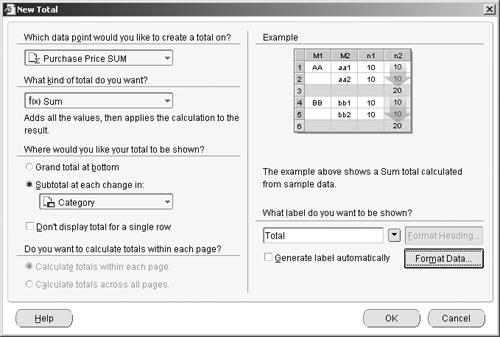
We have already said that we want to total the item purchase price, and in Figure 13.51 we can now add a total to this item as well. As you can see, there are a number of options available to us, such as whether we want a subtotal, the type of sum to perform, and how the data should be formatted. Once again, we can create as many totals as we need for inclusion in our report.
The last step on the wizard is the ability to define a parameter so that the user of the report can be prompted to enter some value. In our example here, we want to see all of the data, but we could use this if, say, we wanted the ability to specify which years data we wanted.
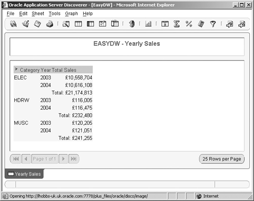
Clicking on the Finish button will display our data. Discoverer will now query our data warehouse directly and show us the results, as shown in Figure 13.52. There we can see the total sales by category for a given year.
Hint
You may have to format the cells of the report to see the data if the numbers are large, because, by default, it uses small numbers.
Note that in order to report this data, we did not have to specify how to join the tables that we selected, because the join information had already been specified in the business area. This is one of the really nice benefits of using Discoverer, because the end user does not have to know about relational joins. The person who created the business area using Discoverer Administration edition has done all of this work behind the scenes. Now all that the user has to do to get the report is select the data of interest, answer the questions on a few screens, and then click the Finish button to request the information.
Now that we have our report, we can customize it to our own requirements by either clicking on the items or selecting from the menu at the top. To change the format of our numbers, if we click on Sheet and then Format, the item can be amended.
If you are interested in how the report is being executed within the database, selecting Sheet, followed by Show SQL, will bring up the SQL Inspector box shown in Figure 13.53. Here you can either view the SQL used to execute the query by clicking on the SQL tab, or, as shown in Figure 13.53, the query execution plan. Here we can see that query rewrite has selected a materialized view to show the results of this query.

Now that we have our report, we may want to look at the data from a different perspective. Discoverer will automatically offer alternative drill down on the data; it’s easy to see if this is possible, by looking for a sideways triangle beside a column.
In Figure 13.52, the column Category has one of these triangles beside it, and clicking on it displays the drop-down list shown in Figure 13.54. Now we have the ability to view the data either by category, or to drill down to the product level. Note that the user did not have to tell Discoverer about how it could report on the data. All this information was previously defined during the setup, so once again the end user needs to know little about how the data is stored in order to get the information requireed.
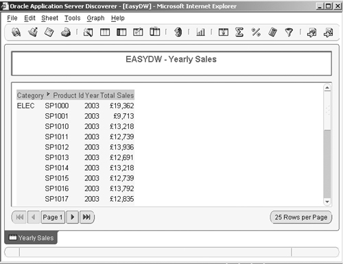
In Figure 13.55, we now see our report with the information at the product level. Because we have a product hierarchy, we can change our report to total by product, instead of by category, simply by selecting product from the drop-down list. Hopefully, now you are beginning to appreciate the benefits of all the setup work that we completed using the Discoverer Administration edition.
So far, we have only viewed our data in a traditional report format, but Discoverer Plus can also represent our data graphically. By answering a few questions using the Graph Wizard, which is started by clicking on the graph icon shown in Figure 13.55, it is possible to create a report similar to the one shown in Figure 13.56.
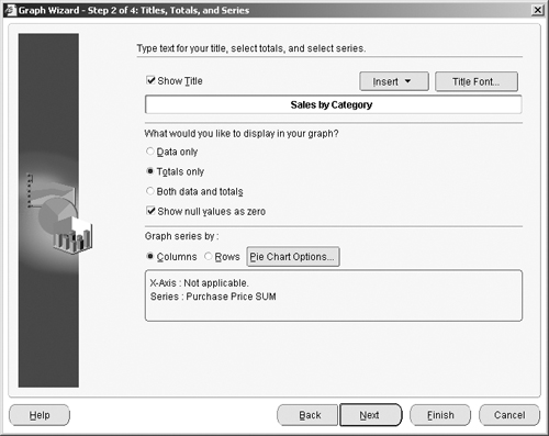
There are over a dozen different types of graphs available from within Discoverer Plus, and you can totally customise the output by adding your own titles and legends. We have decided to use a pie chart to represent our yearly sales, shown in Figure 13.57, which makes it easy for us to see that electrical items were the most popular item.
In this sample Discoverer report, we reported all of the data, but you can select a subset by specifying a condition. What is nice in Discoverer Plus is that you can set up a number of conditions and then select the ones you want for this report. In Figure 13.58, we see one of the screens where you specify these conditions.


There is another screen where you specify the condition, which can be done using quite a complex expression. Here, we can see that we have one conditions defined so that we can select data for a year. Then, when we view the new report in Figure 13.59, we can see that when we restrict the view to just the sales for 2003, electrical is still by far our top-selling item.
There are many more facilities available from Discoverer, but, hopefully, over these few pages, you can now see some of this tool’s capabilities and how ideal this tool is for business-focused end users.
We will discuss Discoverer further in Chapter 14, when we describe how to integrate these reports into Oracle Portal, so that they can be run and viewed from within our browser as part of our Web content.
We have just seen how reports can be generated using tools such as Oracle Discoverer. But if you are looking to create sophisticated reports, which accept data from a variety of sources, can use report templates, and can be published in a variety of formats, such as HTML and PDF, then consider using Oracle Reports 10g.
Oracle Reports 10g will accept data from a variety of sources, including Oracle Database, Oracle Express, Oracle OLAP, XML, JDBC, or even a simple text file. Reports can be presented in a variety of styles and can be enhanced by adding graphs, such as pie charts or bar charts. Each report can be based on predefined templates, or the Template Editor can be used to create your own templates, which means that you can define a standard layout and include, for example, your company logo. Once the report has been defined, it can then be sent to a number of different destinations, which include a file, a printer, email distribution list, or Oracle Portal for inclusion on your corporate Web site. However, the real power of Oracle Reports 10g comes when you can use its powerful Web publishing capabilities, which allow you to create JavaServer Pages (JSP)using Report Builder.
Let us now look at some of the types of reports that we can produce using Oracle Reports.
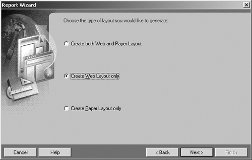
A report can either be constructed manually or by using the Report Wizard, which we will use to guide us through the steps of creating a report. In Figure 13.60, we see one of the first screens, where we are asked to select the type of layout. Since our report is going to be published on our intranet, we have selected the Create Web Layout option. This means that a single report can have two formats, if required: one for paper and another for the Web.
Our next step is to select the type of report we require, as shown in Figure 13.61, where there are a number of options to choose from; a thumbnail sketch of the style is presented next to each radio button. The title of this report will be Monthly Sales by Manufacturer, and the data will be presented in tabular format. Later, we will see examples of reports using the matrix option.

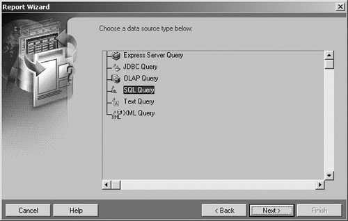
The next step is to define the source of the data; in Figure 13.62, we can see the ways that Oracle Reports allow us to query the data source. In this example, we have chosen to use SQL, but it could just as easily be a query to Oracle OLAP or JDBC.
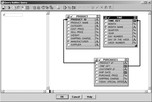
Since we are querying the database, in Figure 13.63 we see there are three methods available for defining the SQL. If you know SQL, then you can type it in manually; otherwise the SQL can be imported from a file, or the Query Builder can construct the query.
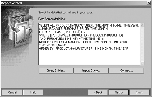
For users not familiar with SQL, use the Query Builder, because it makes defining SQL statements very easy and will certainly save you a lot of time, since all you have to do is select the tables to include in your report and then select the items that are to appear.
Oracle Reports automatically determine how to join the data and creates the required SQL when you leave the query builder. In Figure 13.64, we have selected the PRODUCT, TIME, and PURCHASES tables and have selected some columns from these tables. Note how Oracle Reports have determined how to join the PURCHASES table to the TIME and PRODUCT table.
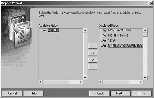
Oracle Reports will now validate our SQL statement, and next we are asked which fields are to appear in the report. In Figure 13.65, we have selected manufacturer, the month name rather than a number, the year, and the total purchase price.
We can now select, in Figure 13.66, whether we require any totals to be computed for data. See how Oracle Reports give us buttons to request for sum, average, count, minimum, maximum, and %total.

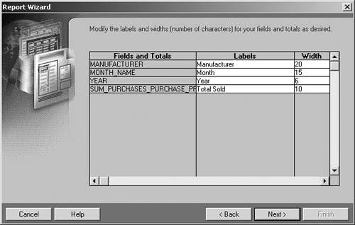
A nice feature in Oracle Reports is the ability to specify how wide the columns should be for our data and what our column headings should be. In Figure 13.67, we are given the option to specify these widths before our report is produced. At this time, column headings can also be defined therefore, we have taken the opportunity to change the heading for Month Name to Month and increase the size of the column for the Manufacturer.
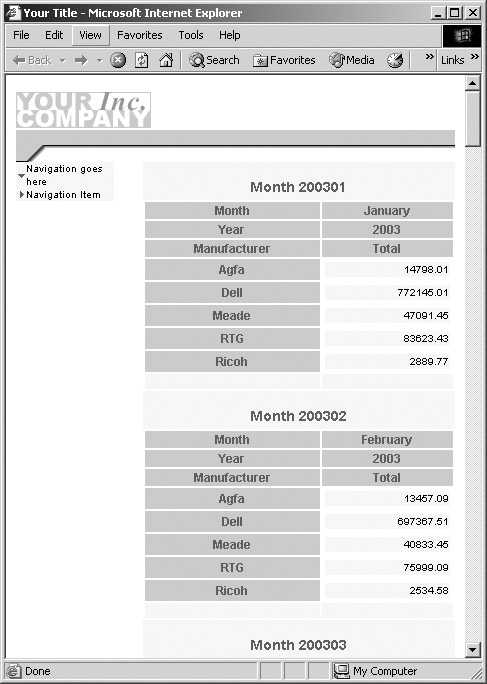
The layout for the report is determined by selecting one of the predefined templates, or you can define your own template. When you’re done, click Finish and you are returned to the Report Builder. Once here you can save the report and then select Program followed by Run Web Layout to actually run the report. Figure 13.68 shows us the actual report as viewed from our browser.

However, this is in its raw format, and it can be customized as required. Therefore, the report layout can be modified to include currency symbols, commas, and decimal points. Other possible changes include changing the fonts, bolding numbers, underline, or italicize text, and you can format numbers to represent a monetary value. You can even add your own logos, graphics, headings and footers, and construct company-specific templates for report layouts.
Report Builder has so many reporting capabilities that once its capabilities are appreciated, it soon becomes apparent how this extremely sophisticated reporting design tool can be used to produce flexible and powerful reports.
The report shown in Figure 13.68 is a very simple report and not that exciting, but it illustrates how to create a report. Let us now look at examples of some more reports that we have created using Oracle Reports from our EASYDW Data Warehouse.
In Figure 13.69, we see an example of a report using the matrix with a group layout, where we can view the total amount that has been purchased for each of our manufacturers for the month of January.
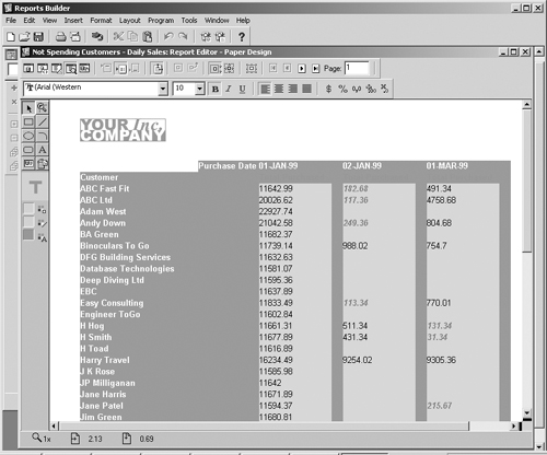
The extensive capabilities of Oracle Reports begin to become apparent when we see how defining a condition on our report can be used to highlight when specified conditions have been reached. In Figure 13.70, we have chosen to highlight in red any customer who spent less than $250. We could even go further and specify a number of conditions, all highlighted with a different color. Therefore, customers spending less than $250 are in red, up to $1,000 in yellow, and over $1,000 in black. Unfortunately, in a black and white book we can’t show this, so the red numbers are in italic.
Once our report has been created, it can then be published in a number of formats. From within Report Builder, we can see the options by clicking File, then Generate, and a list of output formats is displayed, which includes, HTML, PDF, XML, RTF, and Text; we have already seen the HTML layout in Figures 13.68 and 13.69.
By selecting PDF and HTML formats, we have the ability to view the reports using a Web browser. Oracle Reports also allow you to deploy a report to:
File
Printer
OracleAS Portal
Email
Select the type of report that is required, and you will be prompted to specify where the report is to be stored. Optionally, you may also be prompted for database connection information. The report is then run immediately, and the report can be viewed from the location where it is stored.
The report can also be published in OracleAS Portal as a portlet, and we will learn more about publishing data this way in Chapter 14.
In this chapter, we have barely skimmed the surface of what is possible with these three data warehousing tools from Oracle. They are all very powerful and it is strongly recommended that you find out more about these tools; visit http://otn.oracle.com, where there will be demos showing the tools capabilities and very detailed documentation, tutorials, and best practices.