
Query performance tuning is an ongoing process, which is needed throughout the life cycle of any database application. A data warehouse is no exception, and, in fact, good query performance is extremely crucial to the success of any data warehouse. It is important when the application is first designed that the SQL statements are well written and all requisite access structures, such as indexes and materialized views, are created to obtain good execution plans. However, even after the application is deployed, as the data and query workload changes, you will find that you will need to tune the SQL and modify the access structures periodically in order to meet your performance goals.
There are many different reasons why a query may perform poorly. Performance issues may arise due to resource constraints such as inadequate memory or inadequate processing resources. Over time the data distribution may change and the current execution plan may not be optimal. A DBA faces a challenging task of constantly monitoring performance, identifying poorly performing queries, determining the reason for the poor performance, and finally fixing the problem. Therefore, performance tuning can be a very difficult and time-consuming task for even the most experienced DBA.
Fortunately, with Oracle Database 10g, the task of performance tuning is greatly simplified by using several new tools available for this purpose. In this chapter, we will take a look at various aspects of tuning query performance in a data warehouse and the tuning tools available in Oracle Database 10g.
The first step in tuning query performance is to be able to monitor the database and identify queries that are not performing adequately. Oracle Database 10g Enterprise Manager provides a simple interface to monitor such queries. Figure 10.1 shows the Performance page of Oracle Enterprise Manager, which monitors various metrics of performance for the database, such as the waiting sessions, user versus system I/O and instance throughput. To get to this page, after logging into Oracle Enterprise Manager, click on the Performance link at the top of the initial (Home) page.

Near the bottom of this page is a link called Top SQL, which will bring you to the page shown in Figure 10.2. On this page, you can monitor the SQL statements that consumed (or are currently consuming) significant resources in the database. The graph on the top shows the CPU, I/O, and Wait activity in the system over time. The shaded box on the graph corresponds to a five-minute window, and the table below the graph displays the SQL statements that were executed in that window. Click on the rectangle below the graph to move the shaded box to pick a specific five-minute window you are interested in. The page will automatically refresh every 15 seconds by default, though this can be altered by changing the value in the View Data box in the top right of the screen.

The table below the graph in Figure 10.2 shows the SQL statements sorted by a statistic such as by percentage of CPU consumed. Click on the links in the SQL ID column to view the detailed SQL statement, its execution plan, and statistics, as shown in Figure 10.3. From this page it is possible to peruse the execution history and tuning history of the SQL statement.

Once you have identified the poorly performing SQL, you can create a collection, called a SQL Tuning Set, to save these SQL statements persistently in the database. The benefit of creating this collection is that you can keep track of your problematic SQL over a period of time and can use it as input to the tuning tools, SQL Access Advisor and SQL Tuning Advisor, which we will discuss in sections 10.3 and 10.4 respectively.
A SQL Tuning Set can be created either using Oracle Enterprise Manager or by the DBMS_SQLTUNE PL/SQL package.
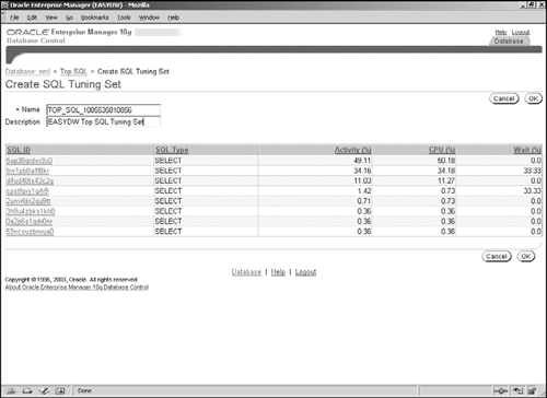
To create a SQL Tuning Set simply select one or more statements from the table in Figure 10.2, and press the Create SQL Tuning Set button to bring up the screen shown in Figure 10.4. Here you can provide a name and description for the SQL Tuning Set and then press OK to create it.
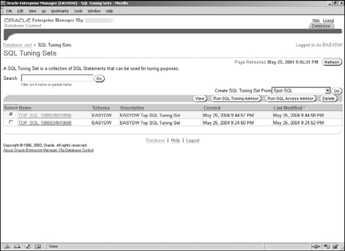
The available SQL Tuning Sets will then be listed in the screen shown in Figure 10.5. From this page, we can manage the SQL Tuning Sets and also run the SQL Access and SQL Tuning Advisors.
SQL Tuning Sets can also be created using the DBMS_SQLTUNE package. The DBMS_SQLTUNE package allows you to create SQL Tuning Sets from the SQL Cache, or any user table as long as it includes some specific columns. In Chapter 5, we discussed how SQL Table functions can be used in the FROM clause instead of an actual table. The SQL Tuning Set procedures provide built-in table functions that allow you to load a workload from the SQL Cache (also called the Cursor Cache), from the Automatic Workload Repository (described in Chapter 11), or from any user table with the SQL statements.
Hint
In order to use the DBMS_SQLTUNE package to create SQL Tuning Sets, you must be familiar with programming using PL/SQL cursors and SQL Table functions.
To avoid creating the SQL Tuning Set with too many statements, you can specify a filter condition restricting the SQL statements to be considered. You can also specify up to three ranking measures used to prioritize (i.e., order) the SQL statements and then request that only the top-N statements or only the ones contributing up to a certain percentage of the ranking measures should be included. When creating a SQL Tuning Set from the SQL Cache, you can use any column from the V$SQL view as a filter condition, and the numeric ones can be used as ranking measures. This should become clearer from the following example, which shows how to create a SQL Tuning Set from the SQL Cache:
DECLARE
   sqlsetname VARCHAR2(30);
   sqlsetcur dbms_sqltune.sqlset_cursor;
BEGIN
   sqlsetname := 'MY_STS_WORKLOAD';
   dbms_sqltune.create_sqlset(sqlsetname, 'SQL Cache STS'),
   OPEN sqlsetcur FOR
     SELECT VALUE(P)
     FROM TABLE(
      dbms_sqltune.select_cursor_cache(
              'SQL_TEXT like ''%purchases%''',
              NULL,
              'CPU_TIME', NULL, NULL, -- ranking measures
              NULL, 10) -- limit to 10
      ) P;
   dbms_sqltune.load_sqlset(sqlsetname, sqlsetcur);
end;
/
In this example, the CREATE_SQLSET procedure creates a SQL Tuning Set with the given name (MY_STS_WORKLOAD) and description (SQL Cache STS). The OPEN statement opens a cursor using the built-in table function, SELECT_CURSOR_CACHE. We have specified a filter, which says that the SQL_TEXT must include the word “purchases,” a ranking measure as CPU_TIME, and a maximum limit of 10 statements.
You can now view the SQL Tuning Set by either using the list in Oracle Enterprise Manager (Figure 10.5) or by using the dictionary views, DBA_SQL_SET and DBA_SQLSET_STATEMENTS, as follows:
select substr(name,1,15) name,substr(owner,1,6) owner,
       substr(sql_text,1,30) description, sql_id
from dba_sqlset d, dba_sqlset_statements s
where id = sqlset_id and name = 'MY_STS_WORKLOAD';

NAME            OWNER  SQL_TEXT                   SQL_ID
--------------- ------ -------------------------  -------------
MY_STS_WORKLOAD EASYDW SELECT t.month, t.year, p  4bw858yjjb11x
MY_STS_WORKLOAD EASYDW SELECT count(distinct pro  4rt9sqw6tnrzz
MY_STS_WORKLOAD EASYDW SELECT sqlset_row (sql_id  5ts120q1a40b5
MY_STS_WORKLOAD EASYDW SELECT VALUE(P) FROM TABL  5z0pw0x58fj88
MY_STS_WORKLOAD EASYDW SELECT VALUE(P) FROM TABL  5zs8b269g338s
...
10 rows selected.
This is a very powerful interface and can be used when you need more functionality and flexibility than are available in the graphical interface in Oracle Enterprise Manager.
Oracle Database 10g Enterprise Manager includes several tools called advisors to aid in performance tuning of the system. The advisors can be launched from a number of locations within Enterprise Manager. However, the most convenient way to find and run any advisor is to follow the Advisor Central link, which can be found at the bottom of the Performance page in Figure 10.1.
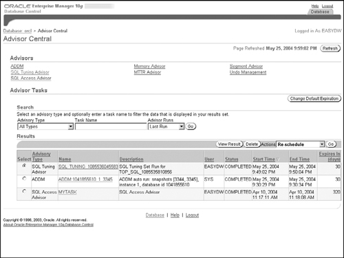
Figure 10.6 shows the Advisor Central page, where you can find links to the following advisors related to query performance tuning:
SQL Access Advisor, which gives advice on index and materialized views
SQL Tuning Advisor, which identifies problems such as missing statistics, possibly bad SQL construction, and so on.
Memory Advisor, for tuning SGA and PGA memory
Additional advisors, such as Segment Advisor and ADDM, are discussed separately in Chapter 11.
Hint
To run the advisors in Oracle Database 10g you must be granted the ADVISOR system privilege, which you will already have if you have the DBA role.
Many of the advisors in Oracle Database 10g, including the SQL Access Advisor and the SQL Tuning Advisor, use a common container known as an Advisor Task to store their tuning parameter settings and the results. On the Advisor Central page, you can monitor currently executing advisor tasks and press the View Result button in Figure 10.6 to look at recommendations of completed tasks.
Hint
By default, a task will be automatically deleted after 30 days, but you can change the expiration date by using the Change Default Expiration button.
We will now look at each of the advisors in detail, starting with the SQL Access Advisor.
One of the most critical aspects of tuning any query is to ensure that it is making use of appropriate access structures such as indexes and materialized views. In Chapter 4, we discussed various indexing techniques for a data warehouse, and in Chapter 9, we saw how you could use a materialized view to answer many different queries using query rewrite. Determining the optimal set of materialized views and indexes to create for the application’s workload of queries is often a difficult exercise. The materialized views must work cooperatively with indexes defined on the base tables and may also need additional indexing. If not done correctly, the application may be slowed down and you could be wasting space and incur overhead to maintain unnecessary structures. The SQL Access Advisor in Oracle Enterprise Manager is an invaluable tool for this purpose. This tool will take a given workload of SQL statements and recommend the ideal set of materialized view and indexes for that workload.
The SQL Access Advisor is available as a wizard in Oracle Enterprise Manager. We recommend using the graphical interface; however, if you prefer to use the command-line interface, you could use the DBMS_ADVISOR PL/SQL package. We will illustrate both of these mechanisms.
Hint
In the previous versions of Oracle, there was a tool called the Summary Advisor, which only recommended materialized views but no indexes. This tool has now been replaced by the SQL Access Advisor, which also recommends indexes.
Figure 10.7 shows the overall flow of the SQL Access Advisor.
The SQL Access Advisor takes as input a workload of SQL statements and some optional tuning parameters. It recommends indexes, materialized views, and any materialized view logs to make the recommended materialized views fast refreshable (see Chapter 7). As mentioned in section 10.2, the analysis parameters and the recommendations resulting from the analysis are stored in an Advisor Task and can be monitored from the Advisor Central page (see Figure 10.6). Note that many of these steps are transparently done for you by the Oracle Enterprise Manager wizard; therefore, you do not need to even know these details unless you plan to use the PL/SQL procedures.
The workload used by the SQL Access Advisor can come from one of the following sources:
A SQL Tuning Set: In section 10.1.1, we discussed how to collect SQL statements from the Top SQL page into a SQL Tuning Set. Once you have created a SQL Tuning Set, you can specify it as a workload source to the SQL Access Advisor.
The SQL Cache: This consists of the current contents of the SQL Cache.
A user-specified table: The workload table may be a table in any schema, which contains the text of the SQL statements.
A Hypothetical Workload: The SQL Access Advisor can generate hypothetical SQL statements using dimension and constraint information from a schema. This can be very useful when you are designing your application schema and cannot run the queries yet.
An Oracle 9i Summary Advisor Workload: If you have used the Summary Advisor in Oracle 9i and have some existing workload, you can reuse this workload for the SQL Access Advisor. To do this, you must provide the SQL Access Advisor with the workload id of the Summary Advisor workload. Note that this option is not available in the graphical interface.
We will now walk through the various steps of the SQL Access Advisor wizard in Oracle Enterprise Manager.
The SQL Access Advisor can be launched from the Advisor Central page shown in Figure 10.6. Alternatively, it may be launched by specifying a SQL Tuning Set as a workload source and then pressing the Run SQL Access Advisor button in Figure 10.5.
If the SQL Access Advisor is launched from Advisor Central, you will first see the screen shown in Figure 10.8, where you must choose a workload source. (When the SQL Access Advisor is launched directly on a SQL Tuning Set, this screen is skipped.)

In Figure 10.8, we have decided to specify a user-defined workload that is contained in the table EASYDW.USER_WORKLOAD. The table used for a SQL Access Advisor workload can be any user table but must have columns, as shown in the following example:
CREATE TABLE user_workload
( MODULE                VARCHAR2(48),
  ACTION                VARCHAR2(32),
  BUFFER_GETS           NUMBER,
  CPU_TIME              NUMBER,
  ELAPSED_TIME          NUMBER,
  DISK_READS            NUMBER,
  ROWS_PROCESSED        NUMBER,
  EXECUTIONS            NUMBER,
  OPTIMIZER_COST        NUMBER,
  LAST_EXECUTION_DATE   DATE,
  PRIORITY              NUMBER,
  SQL_TEXT              CLOB,
  STAT_PERIOD           NUMBER,
  USERNAME              VARCHAR2(30) )
Although this table has many columns, only a couple of them are mandatory columns—namely, the sql_text, which is the complete text of the SQL statement, and the username, which is the name of the user who will execute that SQL statement. The PRIORITY column is a user-settable priority for each SQL statement (1 = HIGH, 2 = MEDIUM, or 3 = LOW). The analysis will make trade-offs in favor of the high-priority SQL statements. If not specified, all statements are treated on an equal footing. All other columns are optional but provide useful statistics for the analysis and will improve the quality of the recommendations.
Alternatively, we can choose the workload source to be a SQL Tuning Set, the current contents of the SQL Cache, or a hypothetical workload generated from a given set of schemas and tables.
At the bottom of Figure 10.8 is a link named Show Advanced Options. Clicking on this link will allow you to set additional options, as shown in Figure 10.9.

Here, you can indicate whether the workload is for a primarily read-only application; in this case, the analysis will ignore the impact of index and materialized view maintenance. Otherwise, the SQL Access Advisor will try to identify the maintenance impact from the DML statements in the workload. Unless you are in the initial design phase of the application, it is wise to allow the Advisor to consider the maintenance impact.
Hint
In order for the SQL Access Advisor to correctly consider maintenance impact of the recommended indexes and materialized views, the workload must include a representative sample of DML statements, such as INSERT, UPDATE, DELETE, and MERGE.
It is also possible to specify if the SQL Access Advisor should consider dropping existing access structures and replacing them with new ones. If you are unsure if your workload covers all relevant SQL for the application, you should choose not to recommend dropping any access structures.
When using a workload source such as the SQL cache, it is possible to have a large number of SQL statements not interesting to the application you are trying to tune. In order to achieve a more focused tuning, it is advisable that you should specify various criteria to narrow down the relevant SQL statements in the workload. By restricting the workload in this manner, the SQL Access Advisor can work in a more focused manner and thereby its analysis would be faster.
In the example, shown in Figure 10.9, we have specified that only SQL statements executed by the user EASYDW and containing tables in the EASYDW schema should be considered for analysis. You could also specify that the top-N most resource consuming SQL be analyzed, or that only SQL from a certain application (specified using the MODULE and ACTION attributes) should be considered.
Once the workload has been chosen, press the Next button to proceed to the screen shown in Figure 10.10, where you can pick various recommendation options for the SQL Access Advisor, as follows.

Recommendation Types: The SQL Access Advisor can recommend Indexes, Materialized Views, or both. If the Indexes option is chosen, it will recommend either B*tree or bitmap indexes. If the Materialized Views option is chosen, it will recommend materialized views and also any materialized view logs required for fast refresh. If both Indexes and Materialized Views are chosen, it will recommend all of these, as well as indexes on the materialized views.
Advisor Mode: The SQL Access Advisor has two modes: Limited and Comprehensive. In the comprehensive mode, it will perform an exhaustive analysis of the entire workload; however, this can take significantly longer to run, depending on the size of the workload. If you would like a quick analysis of the workload, you can specify the limited mode; however, you may not get the best possible recommendations. Use the comprehensive mode as much as possible, unless you have a really large workload.
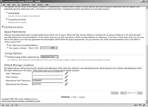
If you click the Show Advanced Options link in Figure 10.10, you can set some additional recommendation options, as shown in Figure 10.11. The advanced options allow you to specify a storage limit (in megabytes) that the recommended access structures should fit within (if created) and also to pick the tablespace and schema where any recommended materialized views and indexes should reside. Note that this information is used when implementing the recommendations, as we will see later.
Pressing the Next button will bring up the screen shown in Figure 10.12, where you can name the advisor task that will contain the results of the analysis. It’s worth choosing a sensible name, because you will need this to retrieve your recommendations from Advisor Central, especially if you wish to come back at a later date and review them. The analysis can be scheduled to execute immediately or at a specified later date.

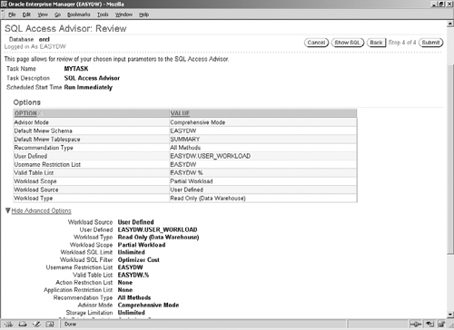
On pressing the Next button, you will see the review screen shown in Figure 10.13, where you can see all your choices at a glance. To make any changes, go back to the previous screens by using the Back buttons.
Once you are satisfied with the settings, you click the Submit button, which will bring you back to Advisor Central; from here you can monitor the status of your job (see Figure 10.6).
Hint
You will need to click the Refresh button on the top right corner in Figure 10.6 to check if the status has changed.
Once the status of the task in Advisor Central indicates Completed, you can select the task and click the View Result button, which will bring you to the recommendations page, shown in Figure 10.14.

There are two ways to view the results of the SQL Access Advisor:
Recommendations View: This view shows each recommendation, consisting of indexes and/or materialized views, along with the estimated performance improvement obtained from that recommendation.
SQL Statement View: This view shows each SQL statement in the workload along with the specific recommendation for that statement and the performance improvement for that statement.
Hint
To switch between these two views choose the required view from the drop-down box labeled View in Figure 10.14. We will look at each of these views in detail.
Figure 10.14 shows the recommendations view, where you can see a bar graph of the estimated improvement in your workload for each recommendation. You can also see the estimated space required to implement that recommendation and the number of SQL statements benefited by that recommendation.
Each recommendation consists of a series of actions to CREATE new materialized views or indexes or to DROP or RETAIN existing ones. There may also be actions to CREATE or ALTER materialized view logs for the recommended materialized views. You can see the actions for each recommendation by clicking on the link in the Recommendation ID column for that recommendation. For example, recommendation ID 4, shown in Figure 10.15, consists of a materialized view and two associated materialized view logs. There is also an auxiliary action to gather statistics on the materialized view once it is created. You can also see the SQL statement(s) that it benefits.
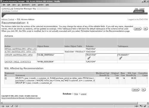
The text of the materialized view can be seen by clicking on the CREATE MATERIALIZED VIEW link in the Action column. Or you can see the SQL for all the actions in a recommendation by clicking the Show SQL button in Figure 10.14. The SQL for Recommendation ID 4 is shown in Figure 10.16.

Recommendation ID 3 consists of an index, as shown in Figure 10.17. Clicking on the CREATE INDEX link will show the detailed columns in the index key.
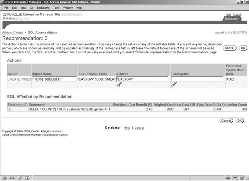
In both Figure 10.15 and Figure 10.17, you can edit the names of the recommended structures and the tablespace and schema where they reside.
The alternate way to view the recommendations is by the SQL statements in the workload, as shown in Figure 10.18.

This view shows the SQL statements that contribute the most improvement in the overall performance of the workload. It also shows the original optimizer cost (as shown by an EXPLAIN PLAN) and the estimated reduction in cost (and thereby increase in performance), if the recommendation were implemented. For example, SQL statement ID 95 was improved by 75 percent. Just as in the recommendations view, you can see the detailed actions in the recommendation by clicking on the links in the Recommendation ID column.
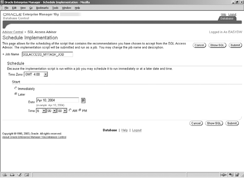
To choose the recommendation(s) you would like to implement simply click on the check boxes in the Select column in Figure 10.14. Creating the access structures can be time consuming and therefore you may want to schedule the implementation during an appropriate maintenance window. Pressing the Schedule Implementation button will bring you to the page shown in Figure 10.19, where you can specify parameters to schedule the implementation. Once you press the Submit button, the implementation job will be scheduled and you will be returned to the Advisor Central page where the status of the job can be monitored.
As we have seen, the SQL Access Advisor wizard is extremely simple to use, and, with a few simple choices, you can tune your application for materialized views and indexes. Next, we will take a brief look at the command-line interface for the SQL Access Advisor.
The SQL Access Advisor can also be run using the PL/SQL procedures in the DBMS_ADVISOR package. The flow for using the command-line interface is the same as the graphical interface. The following example shows the various steps involved in running the SQL Access Advisor on a workload from the SQL Cache.
The first step is to invoke the CREATE_SQLWKLD procedure to create a workload object, which will store the SQL statements in the workload. In this example we are creating a workload object named MY_WORKLOAD.
variable workload_name varchar2(255);
execute :workload_name := 'MYWORKLOAD';
execute dbms_advisor.create_sqlwkld(:workload_name);
You can also specify various criteria to narrow down the workload using the SET_SQLWKLD_PARAMETER procedure. For example, you can specify that the statements in the SQL Cache should be ordered using their ELAPSED_TIME, and only the top-10 statements should be considered.
execute dbms_advisor.set_sqlwkld_parameter(:workload_name,
                                           'ORDER_LIST',
                                           'ELAPSED_TIME'),
execute dbms_advisor.set_sqlwkld_parameter(:workload_name,
'SQL_LIMIT', 10);The next step is to load the SQL statements into the workload. We are loading the workload from the SQL Cache. The filter parameters described in step 2 will be used to determine the statements being loaded.
variable saved_stmts number;
variable total_stmts number;
variable failed_stmts number;

execute dbms_advisor.import_sqlwkld_sqlcache(:workload_name,
                                             'APPEND', 2,
                                             :total_stmts,
                                             :saved_stmts,
:failed_stmts);The next step is to use the CREATE_TASK procedure to create a SQL Access Advisor Task to store the analysis parameters and the recommendations. This is the time to set various parameters such as whether the execution should be INDEX_ONLY and whether the analysis should be limited or comprehensive.
variable task_id number;
variable task_name varchar2(255);

execute :task_name := 'MYTASK';
execute dbms_advisor.create_task('SQL Access Advisor',
                                :task_id, :task_name);

execute dbms_advisor.set_task_parameter(:task_name,
                                        'EXECUTION_TYPE',
'INDEX_ONLY'),Once both the workload and the task are created, they must be linked using the ADD_SQLWLKD_REF procedure.
execute dbms_advisor.add_sqlwkld_ref(:task_name, :workload_name);
Finally, execute the task to generate the recommendations. To obtain a SQL script for the recommended access structures, use the GET_TASK_SCRIPT procedure. This can be run later to create the access structures. Note that you must specify a DIRECTORY object (in this example, ADVISOR_RESULTS) where the script will be placed and you must have write permissions on this directory object.
execute dbms_advisor.execute_task(:task_name);

execute dbms_advisor.create_file(
   dbms_advisor.get_task_script(:task_name),
  'ADVISOR_RESULTS', 'advisor_script.sql'),
The following is an excerpt from a SQL Access Advisor script:
Rem  SQL Access Advisor: Version 10.1.0.1 - Production
Rem
Rem  Username:        EASYDW
Rem  Task:            MYTASK
Rem  Execution date:  19/06/2004 23:59
Rem
...
CREATE BITMAP INDEX "EASYDW"."_IDX$$_0188000E"
    ON "EASYDW"."CUSTOMER"
    ("GENDER")
    COMPUTE STATISTICS;
...The PL/SQL command-line interface provides some features not available in the graphical user interface. One useful feature is templates, which allow you to define a model task, which can then be used as a starting point for other tasks. To create a template, use the same procedure as creating a task and set various analysis parameters. Then, when you need to create a new task with the same parameters, you just create the task from the template.
The following example shows how to create a template named MY_TEMPLATE and then use it to create a new task named MY_TASK.
To create a template, use the CREATE_TASK procedure but set the is_template parameter to TRUE. In this example, the template sets up the default naming conventions for the recommended materialized views and indexes.
variable template_name varchar2(30);
execute :template_name := 'MY_TEMPLATE';
execute dbms_advisor.create_task
    ('SQL Access Advisor',:template_id,
     :template_name,is_template=>'TRUE'),

execute dbms_advisor.set_task_parameter(:template_name,
                                        'INDEX_NAME_TEMPLATE',
                                        'SH_IDX$$_<SEQ>'),

execute dbms_advisor.set_task_parameter(:template_name,
                                        'MVIEW_NAME_TEMPLATE',
'SH_MV$$_<SEQ>'),Another procedure available via the command-line interface but not in the graphical user interface is the ability to analyze a single SQL statement for materialized views and indexes using the QUICK_TUNE procedure. This is a useful tool if you have a problematic SQL query that needs to be resolved immediately and you do not have the time to collect an entire workload and analyze it. Note that if you would like to set any recommendation options for QUICK_TUNE, you must first create a template and then pass it to this procedure.
The following example shows how to run the QUICK_TUNE procedure to analyze a single SQL statement. We use the template MY_TEMPLATE, defined earlier.
variable task_name varchar2(255);
variable sql_stmt varchar2(4000);

BEGIN
   :sql_stmt := ' SELECT count(distinct product_id) as num_cust
                  FROM purchases f, customer c
                  WHERE f.customer_id = c.customer_id and
                        c.gender = :1'

   :task_name :=  'MY_QUICKTUNE_TASK';
   dbms_advisor.quick_tune('SQL Access Advisor',
                           :task_name, :sql_stmt,
                    template=>'MY_TEMPLATE'),
END;
/
Once the procedure completes, you can generate a script just like we did with the previous example.
Unfortunately, due to limited space, we cannot discuss all the procedures in the DBMS_ADVISOR package in detail.
The next section discusses the SQL Tuning Advisor, which is a tool that complements the SQL Access Advisor to tune SQL statements.
It is not always possible to create a new access structure to fix a long-running query. Perhaps it would take too long to create the index or it is not possible to do so except during the maintenance window. Or maybe the problem is that there is a skew in the data distribution, which causes the optimizer to pick a bad execution plan. There may be alternative ways to express the query that are more efficient. In these situations, when you need a quick fix targeted at a specific SQL statement, you should try the SQL Tuning Advisor.
The SQL Tuning Advisor takes as input one or more SQL statements (or a SQL Tuning Set) and gives recommendations to fix each SQL statement using one of the following techniques:
Identifying if a table has changed significantly and its statistics are no longer accurate.
Identifying potential problems in the way the SQL is written. For example, a query may be missing a join condition between two tables, leading to an extremely expensive Cartesian product.
Identifying if the internal estimates used by the cost-based optimizer are off the mark and creating a corrective structure known as a Profile.
The SQL Tuning Advisor is available as a graphical user interface in Oracle Enterprise Manager and as a command-line interface in the DBMS_SQLTUNE PL/SQL package. We will review both these interfaces.
The SQL Tuning Advisor has a simple one-page graphical user interface in Oracle Enterprise Manager. This Advisor can be launched from the Top SQL page, discussed in section 10.1 (see Figure 10.2), by selecting one or more SQL statement(s) and pressing the Run SQL Tuning Advisor button. Alternatively, it is possible to first create a SQL Tuning Set and then launch the SQL Tuning Advisor on it from the screen in Figure 10.5. Once you launch it, you will get a screen similar to the one in Figure 10.20.

As with the SQL Access Advisor, the SQL Tuning Advisor stores its inputs and recommendations in an Advisor Task, for which you may provide a name and description. We recommend you provide a meaningful name or description so you can identify the task in Advisor Central at a later time.
The SQL Tuning Advisor has two modes of analysis: Limited and Comprehensive. In the limited mode, it will spend around one second per statement and do a very quick analysis to look for major problems such as missing statistics. Typically, you would want to run it in the comprehensive mode, where it will attempt to check the optimizer’s cost estimates, check for possible problems in the SQL, look for better execution plans, and so on. In the comprehensive mode, you can specify a maximum time limit for the analysis.
The Advisor can be run immediately or scheduled to run later using the scheduling mechanism in Oracle Enterprise Manager. If you ask to run it immediately, you will get a screen (not shown here) showing the progress of the Advisor until it completes. If you schedule it for later, you can monitor its progress from the Advisor Central page, shown in Figure 10.6, just as you did for the SQL Access Advisor.
Figure 10.21 shows the summary of the recommendations of the SQL Tuning Advisor. For each SQL statement, there will be a check mark indicating the type(s) of recommendations produced. Select any one SQL statement and press the View Recommendation button to see its detailed recommendation. We will now look at a couple of these recommendations.
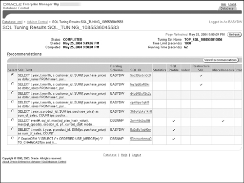
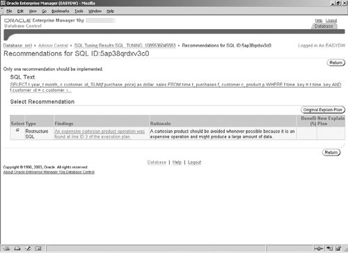
Figure 10.22 shows a recommendation for restructuring a SQL statement. Recommendations in this category require the user to change the SQL text to a different statement, which is not generally equivalent to the original one, but, based on application knowledge, may perform better. For example, suppose a UNION operator were present in the SQL. It is possible that the query would not produce any duplicates (which can only be determined by the application developer), and hence a UNION ALL operator could be used instead and would be much faster. Another common problem is a missing join between two tables, which could be an oversight on the part of the application developer.
Hint
To implement a Restructure SQL type of recommendation, you must be able to physically modify the application or script that launched that SQL statement. Also, care should be taken to ensure that the new SQL produces the same result as the original one, based on your application knowledge.
Note that the SQL Tuning Advisor does not recommend transformations that could transform a SQL into another, better-performing but semantically equivalent SQL statement. This is because the cost-based optimizer will automatically and transparently do these transformations whenever applicable! One example of such a transformation is query rewrite using materialized views, which we discussed in Chapter 9.
Another type of recommendation produced by the SQL Tuning Advisor is a profile, which keeps track of various statistics on the table, as well as predicates and joins in a SQL statement, to assist the optimizer in producing a better execution plan. These statistics are collected by actually running the query on a sample of the data, and by verifying if the optimizer’s estimates match the values found during actual execution. There could be many reasons why the optimizer might produce a bad plan—for example, data skew or stale statistics. The SQL profile will provide information that will allow the optimizer to correct its past mistakes. Once a profile is implemented by pressing the Implement button in Figure 10.23, the optimizer will then automatically use the improved estimates to produce a more efficient execution plan.

Note that sometimes the SQL Tuning Advisor may indicate that a very critical index is missing on a SQL statement. However, this is a very limited analysis and should not be considered as advice to implement the index right away. You should instead run the SQL Access Advisor on that SQL Tuning Set to obtain the comprehensive access structure advice.
In section 10.1.1, we saw how the DBMS_SQLTUNE package can be used to create a SQL Tuning Set. This package also provides PL/SQL procedures to run the SQL Tuning Advisor and to create and manage SQL profiles.
The SQL Tuning Advisor can be run either on a single SQL statement or on a SQL Tuning Set. The following example illustrates how to run this advisor on a single SQL statement. Begin by first using the CREATE_TUNING_TASK procedure to create a task, supplying the SQL statement, and then call EXECUTE_TUNING_TASK to analyze the statement.
variable   task_name     varchar2(30);
declare
  sql_stmt      varchar2(4000);
begin
  -- prepare task to tune
  sql_stmt :=
   'SELECT p.product_id,
          SUM(ps.purchase_price) as sum_of_sales,
          COUNT (ps.purchase_price) as total_sales
   FROM product p, purchases ps
   WHERE ps.customer_id
      not in (select customer_id
              from customer where country = ''US'')
   GROUP BY p.product_id';

  task_name
      := dbms_sqltune.create_tuning_task(sql_text=>sql_stmt);
  -- execute the task created above
  dbms_sqltune.execute_tuning_task(:task_name);
end;
/
The recommendations and any modified query execution plans can then be viewed using the REPORT_TUNING_TASK function, as shown in the following example.
set long 3000
select dbms_sqltune.report_tuning_task(:task_name)
from dual;

----------------------------------------------------------------
GENERAL INFORMATION SECTION
----------------------------------------------------------------
Tuning Task Name   : TASK_497
Scope              : COMPREHENSIVE
...

FINDINGS SECTION (2 findings)
----------------------------------------------------------------
1- SQL Profile Finding (see explain plans section below)
--------------------------------------------------------
A potentially better execution plan was found for this statement.

  Recommendation (estimated benefit: 81%)
  ----------------------------------------
  Consider accepting the recommended SQL profile.
    execute :profile_name :=
        dbms_sqltune.accept_sql_profile(task_name =>'TASK_497'),
...
If the recommendation includes a SQL profile, as in the preceding example, you can use the ACCEPT_SQL_PROFILE procedure to accept the recommendation and create the profile. The next time the SQL statement is executed, the optimizer will use this profile to adjust its estimates when determining an execution plan.
Hint
The REPORT_TUNING_TASK function returns the report as a CLOB column, and hence you must set the long parameter in SQL*Plus and use a SELECT statement to display this column.
Instead of a single statement, if you would like to tune a SQL Tuning Set, you must pass the name of a SQL Tuning Set to the CREATE_TUNING_TASK procedure. The remaining steps are identical to the preceding example.
We have seen how the SQL Access Advisor and SQL Tuning Advisor help find and fix problems with the query performance. However, even with the most optimal plan the performance may be poor if there is a problem during the SQL statement execution. In the next two sections, we will discuss two common problems: insufficient memory and parallel execution problems that can affect query performance.
Good memory configuration is extremely important in the data-intensive applications typical of a data warehouse. The total available physical memory on your system must be properly split between the Operating System, Oracle Shared Global Area (SGA), Process Global Area (PGA), and any other applications running on the system. The SGA is shared by all Oracle server processes. Among other things, the SGA contains the buffer cache, which caches data blocks, and the shared pool, which caches dictionary metadata and compiled cursors. PGA is a separate private memory used by each Oracle server process. PGA memory is used for complex SQL operations, such as sorts, hash joins, and bitmap merges. PGA is also used as buffers for bulk loads and other processing such as PL/SQL and Java. If available physical memory is insufficient to satisfy all these needs, it will result in the Operating System writing pages to disk to free up memory (known as thrashing), causing performance to degrade rapidly.
Oracle Database 10g includes advisors to help tune both PGA and SGA memory. Oracle Enterprise Manager provides a graphical interface to these tools.
PGA memory is the most critical memory parameter for the resource-intensive queries found in a data warehouse. In a data warehouse, PGA memory is used by SQL operations, such as sorts, hash joins, bitmap merges, and bulk loads. The amount of PGA memory used by each operation is called its work area. Due to the memory-intensive nature of these operations, tuning the work areas is very crucial to ensure good query performance. If enough memory is not available, intermediate data may need to be written to temporary segments on disk, which can slow down performance significantly. Prior to Oracle 9i, in order to tune query performance, the DBA had to tune various initialization parameters, such as SORT_AREA_SIZE, HASH_AREA_SIZE, CREATE_BITMAP_AREA_SIZE, and BITMAP_MERGE_AREA_SIZE, to get good performance. However, this was a very difficult and time-consuming process because, the ideal values for these parameters may vary from query to query and may depend on the load on the system. Oracle 9i introduced the automatic PGA memory management feature to ease this burden. Additionally, in Oracle Database 10g the PGA advisor can be used to determine the ideal memory size setting for the system.
Automatic PGA memory management will automatically balance the work area sizes across SQL statements so as to make best use of available memory. The DBA only needs to specify the total amount of memory available for the database instance by setting the initialization parameter, PGA_AGGREGATE_TARGET. To enable automatic memory management the initialization parameter WORKAREA_SIZE_POLICY must be set to AUTO (setting it to MANUAL will revert back to manual memory management).
Hint
The automatic PGA memory management is not available when you use the shared server–based operation in Oracle. For a data warehouse, the number of connections is usually not an issue; hence, it is recommended to use the dedicated server model.
Before we discuss how to tune PGA memory, let us learn how to monitor the PGA memory usage.
The amount of PGA memory allocated and used by each Oracle server process can be seen in the V$PROCESS view, as follows. The PGA_USED_MEM column represents the memory currently in use, PGA_ALLOC_MEM column is total memory currently allocated by the process (some of it may be freed but not yet returned to the operating system), and PGA_MAX_MEM is the maximum ever allocated by that process. In a well-tuned system, every process should be allocating adequate memory but no more than necessary.
SELECT spid, pga_used_mem, pga_alloc_mem, pga_max_mem
FROM v$process;
SPID         PGA_USED_MEM PGA_ALLOC_MEM PGA_MAX_MEM
------------ ------------ ------------- -----------
340                132552        198880      198880
341                135056       3371624     3371624
343               4349880       7570468     7570468
...
The memory used by the work area of SQL statements is seen in the V$SQL_WORKAREA view. You can join to V$SQL to get the complete text for the SQL statements. (We have edited the following output to show only part of the text for lack of space.)
SELECT sql_text, operation_type,
       estimated_optimal_size estsize, last_memory_used
FROM v$sql_workarea w, v$sql s
WHERE w.address = s.address
AND parsing_schema_id = USERENV('SCHEMAID') ;


SQL_TEXT        OPERATION_TYPE    ESTSIZE LAST_MEMORY_USED
--------------- --------------    ------- ----------------
SELECT t.month, GROUP BY (SORT)     56320            49152
SELECT t.month, HASH-JOIN          874496           628736
...
While a query execution is in progress, you can monitor the work area usage in the V$SQL_WORKAREA_ACTIVE view.
-- shows the current workarea usage during an execution
SELECT operation_type, work_area_size, expected_size,
       actual_mem_used
FROM v$sql_workarea_active;

OPERATION_TYPE WORK_AREA_SIZE EXPECTED_SIZE ACTUAL_MEM_USED
-------------- -------------- ------------- ---------------
HASH-JOIN             1087488       1086464          628736
Complex SQL operations need adequate work area memory; otherwise, the operation may need to spill over to temporary segments on disk. The optimal memory size is one that allows the entire operation to be performed entirely in memory. If memory is somewhat less than optimal, then one or more extra passes over the data may be required. A one-pass operation is the next best to the optimal and will perform reasonably well and as work area sizes get larger, may be the typical case. However, a multipass operation will severely degrade performance and should be avoided as much as possible.
Hint
A well-tuned system should have a high percentage of optimal and one-pass executions and very few, if any, multipass executions.
The view V$SQL_WORKAREA_HISTOGRAM can be used to find the distribution of optimal, one-pass, and multipass query executions in your system. The view shows the number of optimal, one-pass, and multi-pass executions for different ranges of work area sizes. For example, in the following query, most executions use work area sizes under 2MB and are able to execute with the optimal amount of PGA memory. There is one query with work areas between 4 and 8 MB, which needed a one-pass execution and two queries with work areas between 8 and 16 MB, which needed a multi-pass execution.
SELECT LOW_OPTIMAL_SIZE LOW, HIGH_OPTIMAL_SIZE HIGH,
       OPTIMAL_EXECUTIONS OPT, ONEPASS_EXECUTIONS Onepass,
       MULTIPASSES_EXECUTIONS multipass
FROM V$SQL_WORKAREA_HISTOGRAM
WHERE TOTAL_EXECUTIONS != 0;

       LOW       HIGH        OPT    ONEPASS  MULTIPASS
---------- ---------- ---------- ---------- ----------
      2048       4095       4712          0          0
     65536     131071         44          0          0
    131072     262143         23          0          0
    262144     524287         20          0          0
    524288    1048575        178          0          0
   1048576    2097151         34          0          0
   4194304    8388607          0          1          0
   8388608   16777215          0          0          2
Now that we understand how to monitor PGA memory usage and identify any multipass executions, let us see how we go about tuning it.
As we mentioned earlier, available physical memory on a system running Oracle must be distributed among the Operating System, SGA, and PGA. For a data warehouse, a good rule of thumb is to set the PGA_AGGREGATE_TARGET initially to about 40 percent to 50 percent of available physical memory and then tune it based on execution of a real workload.
Oracle Database 10g will continuously monitor how much PGA memory is being used by the entire instance by collecting statistics during executions of queries. This information can be seen in the V$PGASTAT view. Using these statistics, it estimates how the performance would vary if the PGA_AGGREGATE_TARGET were set to different values. This information is published in the V$PGA_TARGET_ADVICE view and can be used to tune the PGA_AGGREGATE_TARGET parameter.
Hint
Set the initialization parameter STATISTICS_LEVEL to TYPICAL (default) or ALL; otherwise, the V$PGA_TARGET_ADVICE view is not available.
The following query shows the various statistics in V$PGASTAT:
SELECT  * FROM V$PGASTAT;
NAME                                       VALUE UNIT
------------------------------------------------ ------------
aggregate PGA target parameter          15728640 bytes
aggregate PGA auto target                4194304 bytes
global memory bound                       786432 bytes
total PGA inuse                         16775168 bytes
total PGA allocated                     50482176 bytes
maximum PGA allocated                   59011072 bytes
total freeable PGA memory                6094848 bytes
PGA memory freed back to OS             23986176 bytes
total PGA used for auto workareas         460800 bytes
maximum PGA used for auto workareas      1323008 bytes
total PGA used for manual workareas            0 bytes
maximum PGA used for manual workareas     529408 bytes
over allocation count                        426      <- non zero
bytes processed                         69940224 bytes
extra bytes read/written                62337024 bytes
cache hit percentage                     60.87 percent <- too low

16 rows selected.
The first step is to look at the top two lines of this output: the aggregate PGA target parameter, which is the current setting of PGA_AGGREGATE_TARGET, and the aggregate PGA auto target, which Oracle has calculated as the total memory it can use for SQL work areas. The difference is the estimated memory needed for other processing, such as PL/SQL, and is not tuned by the automatic memory management feature. In our example, the PGA_AGGREGATE_TARGET is 15.7MB, and the total amount available for work areas is 4.2MB. Note that if you find the auto target is much smaller than the PGA_AGGREGATE_TARGET, as is the case in our example, this is one indication that there is not enough PGA memory for work areas and you may need to increase it.
To confirm whether your PGA_AGGREGATE_SETTING is too small, you should look at two quantities - the cache hit percentage and the overallocation count, underlined in the preceding output. The cache hit percentage indicates the percentage of work areas that operated with an optimal allocation of memory. The overallocation count indicates how many times Oracle had to step over the user-defined limit for PGA_AGGREGATE_TARGET, because there was not enough memory available. In a well-tuned system, the overallocation count should be zero, meaning the available PGA memory was sufficient, and the cache hit percentage should be over 80 percent, meaning most queries execute with the optimal amount of memory. If you find that your cache hit percentage is too low or the overallocation count is nonzero, you have insufficient PGA memory. In our example, the cache hit ratio is 61 percent, which is low, and the overallocation count is 426, which is not good.
In these cases you should look at the V$PGA_TARGET_ADVICE view for advice. The view shows the projected values of the cache hit percentage and the overallocation count for various memory sizes. For each memory size, the FACTOR column shows which factor of the current memory setting it is. For example, the row where the FACTOR column is 1 is the current setting, in our example 15.7MB.
select PGA_TARGET_FOR_ESTIMATE PGA_TARGET, PGA_TARGET_FACTOR
FACTOR,
       ESTD_PGA_CACHE_HIT_PERCENTAGE CACHE_HIT_PCT,
       ESTD_OVERALLOC_COUNT OVERALLOC_CNT
from v$pga_target_advice;

PGA_TARGET   FACTOR CACHE_HIT_PCT OVERALLOC_CNT
----------  ------- ------------- -------------
  11796480      .75            50            23
  15728640        1            61            23 <-current setting
  18874368     1.2             61            23
  22020096     1.4             65             2
  25165824     1.6             70             1
  28311552     1.8             80             0 <-minimal needed
  3145728      2               85             0
  47185920     3               87             0
  62914560     4               88             0 <-optimal
  94371840     6               88             0
 125829120     8               89             0

11 rows selected.
When tuning PGA memory, you must ensure that the PGA_AGGREGATE_TARGET is at least set to a value where the overallocation count is zero. Otherwise, there is simply not enough memory for all the work areas. In this example, the minimum memory setting where overallocation count goes to zero is around 28MB. Further, notice that as you increase memory size, the cache hit ratio value increases rapidly up to a point (88 percent for around 63MB in the previous output), and after that it starts to increase more slowly. This point is the optimal value of PGA memory. You must ideally set your PGA memory at or close to this optimal value.
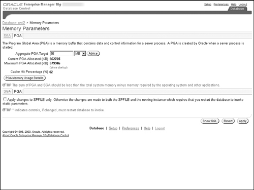
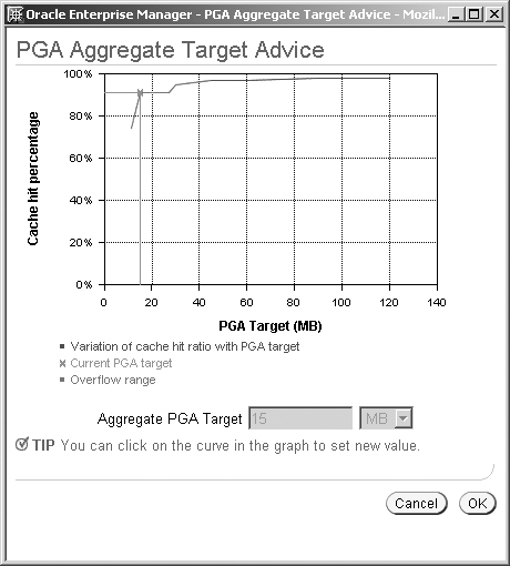
You can see a graphical representation of this view in Oracle Enterprise Manager. From the Advisor Central page (Figure 10.6), if you follow the Memory Advisor link and then click on PGA link, you will see the screen shown in Figure 10.24, which shows the current PGA settings and usage.
From this page, if you click on the Advice button, you will see a line graph as shown in Figure 10.25 with the memory size setting on the X-axis and the cache hit percentage on the Y-axis. You will find that the initial part of the line graph indicates the threshold below which you will see nonzero overallocation count. The optimal value of memory is where this line starts to taper off. The vertical line shows the current setting of the PGA_AGGREGATE_TARGET parameter and can be moved to choose a new setting for this parameter. Once you have chosen a new value, you simply press the OK button and the change will be made.
Hint
At all times, you must ensure that there is adequate physical memory on your system to accommodate increases in the PGA memory for all users. If not, then you will need to decrease the SGA memory size, which may not always be desirable. Increasing PGA memory size without available physical memory means that there will be thrashing, which will only slow the system down.
In the next section, we will discuss how to set the value for the SGA memory.
SGA memory is accessible across all Oracle processes and is used to store various internal control structures, such as compiled cursors and dictionary entries (known as the shared pool), and the buffer cache. The SGA memory setting is not as critical as the PGA in a data warehouse application; however, in any system, it is important to have sufficient SGA memory for smooth functioning. One component of the SGA, known as the large pool, can be important if you are using parallel execution, which was discussed in Chapter 6. Also, you should ensure that you are not allocating too much shared memory, which takes away valuable physical memory that can be used for PGA instead.
Following the Memory Advisor link from Advisor Central, you will come to the SGA Memory Advisor page, shown in Figure 10.26. Here you can see at a glance the allocation of SGA between various pools, such as buffer cache, Java pool, large pool, and so on. On this page you can set the Maximum SGA Size parameter, which will determine the total shared memory allocated when the database starts up. Later, as the database is running, you can adjust the sizes of the individual components, as long as the total does not exceed the specified maximum.

Oracle Database 10g has an Automatic Shared Memory Management feature, which will automatically and dynamically size the various components of the shared memory to adapt to the current workload. To enable this feature, click the Enable button, near the top of Figure 10.26. Note, however, that if you use the automatic feature, you will no longer be able to use the Advisor, since the system will automatically make the changes for you.
You can click the Advice buttons to get advice on setting the shared pool and the buffer cache sizes.
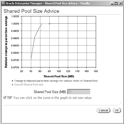
Increasing the shared pool size will improve the time taken to compile a SQL statement. Hence, the shared pool size advice is in the form of a graph, shown in Figure 10.27, with the shared pool size on the X-axis and the expected savings in parse time on the Y-axis. The optimal value is the knee of this graph (i.e., where the graph tapers off). The vertical line shows the current setting of the shared pool, and you can click on the curve to change this setting.
The buffer cache is used to cache frequently used data blocks from disk into memory, thereby speeding up queries. In a data warehouse, many queries involve scanning entire tables, and increasing the size of the buffer cache does not usually speed up these scans. (This is because as new blocks get loaded they displace the earlier blocks and so the next query that needs that earlier block will need to get it from the disk again.) Also, loading of data using SQL*Loader or Parallel DML uses PGA memory and not SGA. So, typically, the size of the buffer cache in a data warehouse would be small compared with that in an OLTP system. You can use the buffer cache advice shown in Figure 10.28, to correctly size your buffer cache so you do not waste too much memory. In this graph, the Y-axis shows the decrease in physical disk blocks read as you increase the buffer cache size shown on the X-axis. Again, the optimal value is around the knee of the graph (i.e., where it starts to flatten out) and you can choose the new setting by clicking on the graph.

Hint
Automatic Shared Memory Management must be disabled in order to see the shared pool and buffer pool advice.
It must be said that, as with all tuning tasks, memory configuration is an iterative process and depends on the workload; therefore, you may need to repeat this process a few times before you get to the optimal settings. However, once you start using automatic PGA and SGA advisors, this process is very straightforward and will ensure that you get the best performance out of your queries.
Parallel execution is one of the most useful features for good query performance in a data warehouse. However, sometimes you may find that your query did not perform as expected even with parallel execution. First and foremost, it is imperative that you have accurate statistics on your tables. If the data has changed significantly and statistics are not updated, the query plan may no longer be optimal. If statistics are not the problem, it may be that the optimizer did not generate a parallel execution plan for your query. It is also possible that resource constraints forced the query to be executed serially.
In this section, we will discuss some of the problems that can occur with parallel execution and how to identify and fix them.
The first step when troubleshooting parallel execution is to check for possible problems with the query plan. You can use the EXPLAIN PLAN facility (discussed in Chapter 6) to display the parallel query execution plan. Note that you must use the script utlxplp.sql to display the plan. The following example shows the parallel execution plan for the same query used in Chapter 6. We have formatted the plan to show only columns related to parallel execution, for lack of space.
EXPLAIN PLAN FOR
SELECT t.month, t.year, p.product_id,
       SUM (purchase_price) as sum_of_sales,
       COUNT (purchase_price) as total_sales,
       COUNT(*) as cstar

FROM time t, product p, purchases f
WHERE t.time_key = f.time_key AND
      f.product_id = p.product_id
GROUP BY t.month, t.year, p.product_id;
                                 ----------
------------------------------------------------------------------
|Id|Operation                    |Name     |  TQ |IN-OUT|PQDistrib|
------------------------------------------------------------------
| 0|SELECT STATEMENT             |         |     |      |         |
| 1|PX COORDINATOR               |         |     |      |         |
| 2| PX SEND QC (RANDOM)         |:TQ10003 |Q1,03| P->S |QC (RAND)|
| 3|  SORT GROUP BY              |         |Q1,03| PCWP |         |
| 4|   PX RECEIVE                |         |Q1,03| PCWP |         |
| 5|    PX SEND HASH             |:TQ10002 |Q1,02| P->P |HASH     |
| 6|     HASH JOIN               |         |Q1,02| PCWP |         |
| 7|      PX RECEIVE             |         |Q1,02| PCWP |         |
| 8|       PX SEND BROADCAST     |:TQ10000 |Q1,00| P->P |BROADCAST|
| 9|        PX BLOCK ITERATOR    |         |Q1,00| PCWC |         |
|10|         TABLE ACCESS FULL   |TIME     |Q1,00| PCWP |         |
|11|      HASH JOIN              |         |Q1,02| PCWP |         |
|12|       PX RECEIVE            |         |Q1,02| PCWP |         |
|13|        PX SEND BROADCAST    |:TQ10001 |Q1,01| P->P |BROADCAST|
|14|         PX BLOCK ITERATOR   |         |Q1,01| PCWC |         |
|15|         INDEX FAST FULL SCAN|PRODUCT  |Q1,01| PCWP |         |
|  |                             |_PK_INDEX|     |      |         |
|16|       PX BLOCK ITERATOR     |         |Q1,02| PCWC |         |
|17|        TABLE ACCESS FULL    |PURCHASES|Q1,02| PCWP |         |
------------------------------------------------------------------
The first thing to note is that if you ignore the rows prefixed with a PX, the plan is the same as the serial plan seen earlier in Chapter 6! The PX rows for each operation indicate how that operation has been parallelized. For instance, the PX BLOCK ITERATOR row for id 16 indicates that the scan of the PURCHASES TABLE has been parallelized at the block granule. The TQ column and the :TQxxxx names refer to communication pipes between the query coordinator process and the parallel execution servers. The IN-OUT columns indicate which processes are involved in the communication at each stage. The important thing to note for this column is that as long the value is P->P, PCWC, or PCWS it implies that operation is in parallel. However, if you see P->S or no value at all, it means that at that point the operation is serial. Typically, you will see P->S when the coordinator collects results from all the slaves. This column can be used to check if your plan is using parallel execution throughout or if some operation is being unexpectedly serialized. If you find that an operation that can be parallelized, such as a table scan, a join, or a sort, is executing serially, then there may be a problem with the execution plan.
If you find that an operation is serial where it could be parallel, check your parallel execution setup and ensure that the tables and indexes have statistics. Check if some user-defined function or aggregate (discussed in Chapter 6) is preventing parallel execution. Run the SQL Tuning Advisor to see if your query can be tuned further. For instance, if your query involves subqueries, it may be possible to express the query using a join instead.
Finally, the last column in the plan display, PQ Distrib, is the method used by parallel execution to distribute rows of a table among the slaves: broadcast, meaning all rows are sent to all slaves; hash, meaning a hash function is used to distribute the rows; and random, meaning the rows are distributed randomly among the slaves. If the table data is skewed so that there are more rows with one value than another, or if there are very few distinct values, then this can result in some slaves having more work to do than others. In this case, the PX_DISTRIBUTE hint can be used to alter the distribution method chosen by the optimizer.
If the query plan looks good, then the problem is likely due to lack of some resource.
You can find some useful execution statistics in various dynamic performance views such as V$SYSSTAT, V$PX_SESSION and V$PX_PROCESS_SYSSTAT.
Hint
Corresponding to every V$ view is a GV$ view. The V$ views only give statistics for the current instance. If you are using Real Application Clusters, you will have multiple instances and will need to use the GV$ views. The GV$ views give the statistics for all the instances and therefore have an extra column, INST_ID.
The view V$SYSSTAT keeps cumulative statistics about the Oracle instance from the time of database startup. The following query can be used to query the statistics related to parallel execution. From this you can tell if your queries are being parallelized with the desired degree of parallelism or if they are being downgraded due to resource contention. If you find this to be the case, you may need to limit the number of concurrent users or identify whether there is some high-load SQL statement that is taking up a lot of the parallel execution servers. In the following output, the rows marked with an asterisk indicate that some statements did not execute with the requested degree of parallelism.
SELECT ss.value, ss.name
FROM v$sysstat ss
WHERE UPPER(ss.name) like '%PARALLEL%'
   or UPPER(ss.name) like '%PX%';

     VALUE NAME
---------- -----------------------------------------------
         5 DBWR parallel query checkpoint buffers written
         8 queries parallelized
         0 DML statements parallelized
         0 DDL statements parallelized
         8 DFO trees parallelized
         4 Parallel operations not downgraded
         0 Parallel operations downgraded to serial
         0 Parallel operations downgraded 75 to 99 pct
       * 1 Parallel operations downgraded 50 to 75 pct
       * 1 Parallel operations downgraded 25 to 50 pct
       * 3 Parallel operations downgraded 1 to 25 pct
    151171 PX local messages sent
    151084 PX local messages recv'd
         0 PX remote messages sent
         0 PX remote messages recv'd
15 rows selected.
The V$PX_SESSION view can be used to figure out which parallel execution servers are working together on a query. QCSID is the session id of the coordinator and there is one row for each slave process, with SID being the session id of the slave process. One useful piece of information in this view is the requested and actual degree of parallelism for the operation. If the requested degree is more than the actual, then you have a resource shortage. In this example, the requested degree is 8 and the actual degree is 7, which indicates a shortage of parallel execution servers.
SELECT QCSID, SID, DEGREE "Degree", REQ_DEGREE "Req Degree"
FROM V$PX_SESSION
ORDER BY QCSID, QCINST_ID, SERVER_GROUP, SERVER_SET;
     QCSID        SID     Degree Req Degree
---------- ---------- ---------- ----------
       142        122          7          8
       142        140          7          8
       142        124          7          8
...
Finally, the V$PX_PROCESS_SYSSTAT gives information about the status of the parallel execution servers and statistics about memory and buffer allocations. The Highwater, or HWM, figures represent the maximum concurrent usage for that resource and give you an idea whether the resource is being maximally used at the present time. Specifically, if the Servers Highwater value is equal to PARALLEL_MAX_SERVERS, it means that all the parallel execution server processes were in use concurrently at some point in time. In this case, you should consider increasing this parameter, if you have the processing capacity.
select * from V$PX_PROCESS_SYSSTAT;

STATISTIC                           VALUE
------------------------------ ----------
Servers In Use                         28
Servers Available                       2
Servers Started                        34
Servers Shutdown                        4
Servers Highwater                      30
Servers Cleaned Up                      0
Server Sessions                        92
Memory Chunks Allocated                 9
Memory Chunks Freed                     2
Memory Chunks Current                   7
Memory Chunks HWM                       9
Buffers Allocated                    1234
Buffers Freed                         856
Buffers Current                       378
Buffers HWM                           387
Oracle recommends configuring the LARGE_POOL_SIZE parameter when using parallel execution. This memory pool is used to store the message buffers for communication between parallel execution processes. If the product of Buffers HWM and the initialization parameter PARALLEL_MESSAGE_BUFFER_SIZE is much less than the parameter LARGE_POOL_SIZE, you should consider increasing this parameter setting.
You should also consider using the Oracle Resource Manager to create resource plans to limit resource usage for each user or application. We cannot stress enough that for parallel execution to be effective, it is important to have sufficient hardware capacity; otherwise, no amount of tuning can improve your performance.
You have successfully tuned and deployed your data warehouse application and everything is running perfectly. Then you apply a new patch to the underlying database and suddenly everything slows down and the users start complaining. What happened? Well, the most likely explanation is that the optimizer chose a different strategy for the query execution, which it believes is better but in reality is worse. This can happen for many reasons, including skewed data distribution, different optimizer statistics, or a new default setting for some initialization parameter. Thus, anytime you do a software upgrade, or after statistics get updated, there is a risk that a query execution plan may change and the query may take longer to run.
To mitigate this problem, Oracle has a feature called plan stability. This allows you to create an object called a stored outline for a SQL statement, which keeps a record of the execution plan for that query. When a query is issued, if there is an outline for that query, Oracle will try to reproduce the same execution plan as stored in the outline.
You can instruct Oracle to create outlines for all SQL statements or for specific SQL statements. Outlines can be grouped together into categories to better organize and manage them.
The schema where outlines will be created must have the CREATE ANY OUTLINE system privilege.
To create stored outlines for all SQL statements you must set the parameter CREATE_STORED_OUTLINES to TRUE or specify a category name to group the outline into. In the following example, we are setting the category name to EASYDW_CAT.
ALTER SESSION SET CREATE_STORED_OUTLINES = easydw_cat;
Once you set this, outlines will automatically be created for every SQL statement and associated with the given category (if specified). This is an easy way to create the outlines, but it may result in a large number of outlines. Typically, just before upgrading to a new database version, you would turn this parameter on, leave the application running for some period of time to create outlines, and then turn the parameter off by setting CREATE_STORED_OUTLINES to false.
Alternatively, you can create stored outlines for specific SQL statements using the CREATE OUTLINE statement. In the following example, we are creating an outline named CUST_OUTLN under the category CUST_PURCHASES_CAT.
CREATE OUTLINE cust_outln FOR CATEGORY cust_purchases_cat
ON
SELECT count(distinct product_id) as num_cust
FROM purchases f, customer c
WHERE f.customer_id = c.customer_id and
c.gender = 'F';To use stored outlines, you must set the parameter USE_STORED_OUTLINES to true or to a category name (which you specified when you created the outlines). When Oracle compiles a SQL statement, it looks to see if there is an outline for a query with exactly the same text as the query. If it finds one, then the information stored in the outline is used to control the execution plan generated for the query.
ALTER SESSION SET USE_STORED_OUTLINES = easydw_cat;
To check if a query used an outline, you can run the EXPLAIN PLAN utility to see the execution plan of the query. The output will indicate the name of the outline used, if any. You can also view the available outlines and their usage using the USER_OUTLINES dictionary view, as shown in the following example.
NAME       USED SQL_TEXT
---------- ---- --------------------------------
CUST_OUTLN USED SELECT count(distinct product_id
Hint
Using an outline does not guarantee that you will get the identical execution plan. For example, if the outline referred to an index that was later dropped, you would obviously not be able to use the execution plan using that index. Also, some initialization parameter settings may take precedence over outlines—for example, if you set query_rewrite_enabled to false, Oracle will not use a materialized view even if you had an outline using it.
As you can see, plan stability is extremely simple to use and can be a very valuable tool to ensure that query performance remains predictable. After your application has been tuned adequately, consider creating some outlines for your important queries. Once they have been created and stored in the database, it is not necessary that you use them all the time. Instead, they can be kept in case of emergency and enabled only in the event of performance degradation. Outlines are also useful when building applications that are deployed at a number of sites to ensure the same query execution plan is chosen for all users.
In this chapter, we discussed various aspects of query performance tuning. Oracle Database 10g provides tuning tools such as the SQL Access Advisor and SQL Tuning Advisor, which can be invaluable assistants to a DBA in simplifying the ongoing tasks of performance tuning. With these tools you can create index and materialized views to speed up your queries and also improve the optimizer’s ability to create good execution plans, using profiles. We also discussed how you could find and fix some common parallel execution problems and tune the PGA memory so that the queries execute with the optimal memory required. Finally, we discussed how you can use plan stability to keep the query performance predictable over time.
Query performance tuning is just one of the tasks faced by a DBA when managing a warehouse. Chapter 11 looks at the larger scope of managing a data warehouse and the tools and features Oracle Database 10g provides for this purpose.