Partitioning should be considered for large tables, over 2GB in size. Partitioning is also useful for tables that have mostly read-only historical data. A common example is a fact table containing a year’s worth of data, where only the last partition has data that can change and the other partitions are read-only.

A table can be partitioned using a column called the partition key, whose value determines the partition into which a row of data will be placed. In general, any column of numeric, character, or date data type can be used as a partition key; however, you cannot partition a table by a LONG or LOB column.

All partitions of a table or index have the same logical attributes, such as columns and constraints, but can have different physical attributes, such as the tablespace they are stored in.

Oracle Database 10g provides several methods to partition your tables:

We will now discuss each of these in detail.

One of the most frequently used partitioning methods is range partitioning, where data is partitioned into nonoverlapping ranges of data. In range partitioning, each partition is defined by specifying the upper bound on the values that the partition-key column can contain. As each row gets inserted into the table, it is placed into the appropriate partition based on the value of the partition key column. Range partitioning is especially suitable when the partition-key is continuous, such as time. It allows the optimizer to perform partition pruning for queries asking for a specific value or a range of partition-key values.

Figure 4.1 shows a table partitioned by range, using the TIME_KEY as the partition key. Each partition has data for one month and is stored in its own tablespace.

Figure 4.1. Range Partitioning by MONTH

The SQL that would create this partitioned table is shown in the following code. The VALUES LESS THAN clause specifies the upper bound on the partition-key values in that partition. The lower bound is specified by the VALUES LESS THAN clause of the previous partition, if any. In our example, the purchases_feb_2003 partition has data values with time_key >= ‘01-FEB-2003’ and < ‘01-MAR-2003’.

CREATE TABLE easydw.purchases
(product_id             varchar2(8),
 time_key               date,
 customer_id            varchar2(10),
 purchase_date          date,
 purchase_time          number(4,0),
 purchase_price         number(6,2),
 shipping_charge        number(5,2),
 today_special_offer    varchar2(1))
PARTITION by RANGE (time_key)
 (partition purchases_jan2003
     values less than (TO_DATE('01-FEB-2003', 'DD-MON-YYYY'))
     tablespace purchases_jan2003,
  partition purchases_feb2003
     values less than (TO_DATE('01-MAR-2003', 'DD-MON-YYYY'))
     tablespace purchases_feb2003,
  partition purchases_mar2003
     values less than (TO_DATE('01-APR-2003', 'DD-MON-YYYY'))
     tablespace purchases_mar2003,
  partition purchase_catchall
     values less than (MAXVALUE)
     tablespace purchases_maxvalue);

Notice that the last partition in the PURCHASES table has a special bound called MAXVALUE. This is an optional catchall partition, which collects all rows that do not correspond to any defined partition ranges.

With range partitioning, it is possible to end up with a situation where the data is not evenly divided among the partitions. Some partitions may be very large and others small. For example, if the data was partitioned by month and some months experience peak sales (e.g., December due to Christmas), then this would result in partitions that are very different in size. When the data is skewed in this way, “hot spots” form where there is contention for resources in one area.

Hash partitioning reduces this type of data skew by applying a hashing function to the partitioning key. The resulting output value is used to determine which partition to store the row in. So instead of partitioning by MONTH, if we hash partition the PURCHASES table by PRODUCT_ID, all rows for a month would get scattered across several partitions, as shown in Figure 4.2, resulting in more evenly sized partitions.

Figure 4.2. Hash Partitioning by Product

Notice that all products with the same PRODUCT_ID fall into the same partition however, the user has no control or knowledge of which products go into which partitions. You can only specify how many partitions you would like.

In the following code, we illustrate the SQL required to create a hash-partitioned table with four partitions using the PRODUCT_ID column as the partitioning key.

CREATE TABLE easydw.purchases
 (product_id             varchar2(8),
  time_key              date,
  customer_id           varchar2(10),
  purchase_date         date,
  purchase_time          number(4,0),
  purchase_price         number(6,2),
  shipping_charge        number(5,2),
  today_special_offer    varchar2(1))
PARTITION BY HASH(product_id)
PARTITIONS 4;

With hash partitioning, the optimizer can perform partition pruning if the query is asking for a specific value or values of the partition key. For example, if we had a query based on a specific product, such as “How many tents did we sell each month?” the optimizer could determine which partition to look in to find “Tents.” However, if we had a query that asked for a range of product ids, we would need to search all partitions.

Because hash partitioning reduces contention on the table, you may find hash partitioning used in OLTP systems. However, recall that there is no logical correlation between the partition and the values stored in it. In a data warehouse maintenance operations often require knowledge of the data values, such as deleting or archiving old data from the table. Hence, in a data warehouse, hash partitioning is seldom used alone but instead is used in conjunction with range partitioning. This technique is known as Composite Partitioning and is discussed in section 4.2.5.

In some cases, it may not be convenient to organize data into ranges of values. The data may not have a natural partitioning key such as time. For business reasons, values that are far apart may need to be grouped together. For instance, if we have sales data for the states of the United States, it is not very easy to put data for all states in a given region, such as the Northeast, into the same partition using range or hash partitioning. The partitioning technique to solve this problem is List Partitioning, which allows data to be distributed according to discrete column values. Figure 4.3 shows an example of a list-partitioned table by discrete values of states.

Figure 4.3. List Partitioning by State

The following SQL statement uses list partitioning to organize the sales data by region. The last partition, which uses the keyword DEFAULT, is a catchall partition that captures the rows that do not map to any other partition.

CREATE TABLE easydw.regional_sales
(state                 varchar2(2),
 store_number          number,
 dept_number           number,
 dept_name             varchar2(10),
 sales_amount          number (6,2)
)
PARTITION BY LIST(state)
(
  PARTITION northeast   VALUES ('NH', 'VT', 'MA', 'RI', 'CT'),
  PARTITION southeast   VALUES ('NC', 'GA', 'FL'),
  PARTITION northwest   VALUES ('WA', 'OR'),
  PARTITION midwest     VALUES ('IL', 'WI', 'OH'),
  PARTITION west        VALUES ('CA', 'NV', 'AZ'),
  PARTITION otherstates VALUES (DEFAULT));

List partitioning allows the query optimizer to perform partition pruning on queries that ask for specific values of the partitioning key. For instance, a query requesting data for Massachusetts (MA) or New Hampshire (NH) only needs to access the Northeast partition.

Oracle provides a two-level partitioning scheme known as composite partitioning to combine the benefits of two partitioning methods. In composite partitioning, data is divided into partitions using one partitioning scheme and then each of those partitions is further subdivided into subpartitions using another scheme. Currently, Oracle supports the following two types of composite partitioning schemes:

Range-Hash Partitioning

We mentioned earlier that hash partitioning does not allow a user control over the distribution of data. On the other hand, range partitioning suffers from the potential problem of data skew. Range-Hash composite partitioning combines the benefits of both range and hash partitioning. The data is first partitioned by range and then further subdivided into subpartitions by using a hash function. When partitioning by date, the last partition is often a “hot spot.” Subpartitioning can eliminate such hot spots by placing each subpartition on different tablespaces and on different physical devices if required, thereby reducing the I/O contention.

In Figure 4.4, the data is first partitioned by the month and then further partitioned by the product. Each partition has four subpartitions.

Figure 4.4. Range-Hash Composite Partitioning

The SQL to create a composite partitioned table is shown in the following code. The STORE IN clause allows you to name the tablespace where each subpartition will reside. Each subpartition has been stored in its own tablespace.

CREATE TABLE easydw.purchases
 (product_id                  varchar2(8),
  time_key                    date,
  customer_id                 varchar2(10),
  purchase_date               date,
  purchase_time               number(4,0),
  purchase_price              number(6,2),
  shipping_charge             number(5,2),
    today_special_offer         varchar2(1))
PARTITION by RANGE (time_key)
SUBPARTITION BY HASH(product_id)
SUBPARTITIONS 4
   (partition purchases_jan2003
     values less than (TO_DATE('01-FEB-2003', 'DD-MON-YYYY'))
        STORE IN (purchases_jan2003_1,
                  purchases_jan2003_2,
                  purchases_jan2003_3,
                  purchases_jan2003_4),
    partition purchases_feb2003
     values less than (TO_DATE('01-MAR-2003', 'DD-MON-YYYY'))
        STORE IN (purchases_feb2003_1,
                  purchases_feb2003_2,
                  purchases_feb2003_3,
                  purchases_feb2003_4),
    partition purchases_mar2003
     values less than (TO_DATE('01-APR-2003', 'DD-MON-YYYY'))
       STORE IN  (purchases_mar2003_1,
                  purchases_mar2003_2,
                  purchases_mar2003_3,
                  purchases_mar2003_4));

To avoid data skew it is recommended that the number of hash subpartitions be a power of 2.

CREATE TABLE sales
(state                  varchar2(2),
 store_number           number,
 dept_number            number,
 dept_name              varchar2(10),
 sales_amount           number (6,2),
 sale_date              date,
 item_number            number (10)
)
PARTITION BY RANGE (sale_date)
SUBPARTITION BY LIST(state)
SUBPARTITION TEMPLATE
(
 SUBPARTITION "NorthEast"
    VALUES ('NH', 'VT', 'MA', 'RI', 'CT')
     TABLESPACE sales_ne,
 SUBPARTITION "SouthEast"
     VALUES ('NC', 'GA', 'FL')
     TABLESPACE sales_se,
 SUBPARTITION "NorthWest"
     VALUES ('WA', 'OR')
     TABLESPACE sales_nw,
  SUBPARTITION "MidWest"
     VALUES ('IL', 'WI', 'OH')
     TABLESPACE sales_mw,
 SUBPARTITION "West"
     VALUES ('CA', 'NV', 'AZ')
     TABLESPACE sales_w)
(PARTITION sales_jan_2003
    VALUES LESS THAN (TO_DATE('01-FEB-2003', 'DD-MON-YYYY')),
  PARTITION sales_feb_2003
     VALUES LESS THAN (TO_DATE('01-MAR-2003', 'DD-MON-YYYY')),
  PARTITION sales_mar_2003
     VALUES LESS THAN (TO_DATE('01-APR-2003', 'DD-MON-YYYY')));

SELECT partition_name, subpartition_name
FROM user_tab_subpartitions
WHERE table_name = 'SALES';
PARTITION_NAME              SUBPARTITION_NAME
--------------------------- -------------------------
SALES_JAN_2003              SALES_JAN_2003_NorthEast
SALES_JAN_2003              SALES_JAN_2003_SouthEast
SALES_JAN_2003              SALES_JAN_2003_NorthWest
SALES_JAN_2003              SALES_JAN_2003_MidWest
SALES_JAN_2003              SALES_JAN_2003_West
SALES_FEB_2003              SALES_FEB_2003_NorthEast
SALES_FEB_2003              SALES_FEB_2003_SouthEast
SALES_FEB_2003              SALES_FEB_2003_NorthWest
SALES_FEB_2003              SALES_FEB_2003_MidWest
SALES_FEB_2003              SALES_FEB_2003_West
...

A partition key used for range or hash partitioning can have multiple (up to 16) columns. Multicolumn partitioning should be used when the partitioning key is composed of several columns and subsequent columns define a finer granularity than the preceding ones. We will illustrate this with an example using range partitioning.

The following SQL creates a table with range partitioning using a multicolumn partitioning key, TIME_KEY, PRODUCT_ID.

CREATE TABLE easydw.purchases
(product_id                 varchar2(8),
 time_key                   date,
 customer_id                varchar2(10),
 purchase_date              date,
 purchase_time              number(4,0),
 purchase_price             number(6,2),
 shipping_charge            number(5,2),
 today_special_offer        varchar2(1))
PARTITION by RANGE (time_key, product_id)
 (
  partition purchases_jan2003_100
   values less than (TO_DATE('31-JAN-2003','DD-MON-YYYY'), 100)
   tablespace purchases_jan2003_100,
  partition purchases_jan2003_200
   values less than (TO_DATE('31-JAN-2003','DD-MON-YYYY'), 200)
   tablespace purchases_jan2003_200 ,
  partition purchases_feb2003_all
   values less than (TO_DATE('28-FEB-2003','DD-MON-YYYY'), 100)
   tablespace purchases_feb2003,
  partition purchases_mar2003_all
   values less than (TO_DATE('31-MAR-2003','DD-MON-YYYY'), 100)
   tablespace purchases_mar2003
);

To understand how data gets mapped to partitions, let us now insert some data values into this table and see which partitions they go into.

insert into purchases (product_id, time_key)
       values (1, TO_DATE('15-JAN-2003', 'DD-MON-YYYY'));

insert into purchases (product_id, time_key)
       values (150, TO_DATE('15-JAN-2003', 'DD-MON-YYYY'));

insert into purchases (product_id, time_key)
       values (101, TO_DATE('31-JAN-2003', 'DD-MON-YYYY'));

The first row obviously goes into the first partition. Intuitively, you would expect that the second row with TIME_KEY = 15-JAN-2003 and PRODUCT_ID = 150 would go into the second partition. However, this is not the case. Let us issue the following query, which shows all the rows that belong to the first partition. (Note the special PARTITION syntax, which allows you to query data from a specific partition by specifying the partition name.)

SELECT product_id, time_key
FROM purchases partition(purchases_jan2003_100);

PRODUCT_ID  TIME_KEY
----------  -----------
1            15-JAN-2003
150          15-JAN-2003

What we find is that the row is actually in the first partition! The reason for this is that the condition checked for the first partition is in fact the following:

   (TIME_KEY < '31-JAN-2003')
OR (TIME_KEY = '31-JAN-2003' AND PRODUCT_ID < 100).

In other words, the condition on the second column is checked only if the value of the first column is equal to the partition bound. Therefore, in our example, the row with TIME_KEY = ‘15-JAN-2003’ actually falls into the first partition. On the other hand, the third row, which has TIME_KEY = ‘31-JAN-2003’ and PRODUCT_ID = 101, does not satisfy the condition for the first partition. It will go into the second partition, as shown by the following query:

SELECT product_id, time_key
FROM purchases partition(purchases_jan2003_200);

PRODUCT_ID  TIME_KEY
----------  -----------
101         31-JAN-2003

This is because the condition for the second partition is:

(time_key = '31-JAN-2003' and product_id < 200)

Multikey range partitioning can be useful if you have one TIME_KEY value with lots of PRODUCT_ID values (e.g. lot of purchases may be made on Christmas eve). In this case, you can use the second column to distribute the data for the specific TIME_KEY value into multiple partitions.

Range partitioning with a multicolumn partition key must not be confused with Range-Range composite partitioning. As of the time of writing, Oracle does not support Range-Range composite partitioning. If it were supported, the row with TIME_KEY = 15-JAN-2003 and PRODUCT_ID = 150 would have mapped to the second partition in the previous example.

Now that we know all the partitioning methods, let us briefly review how you would go about choosing the partitioning method.

Range partitioning should be used when your table has a continuous key, such as time. List partitioning is ideal for tables where you would like to place specific discrete values in one partition. Hash partitioning distributes data uniformly among all partitions and may be used alone or in combination with Range partitioning to avoid hot spots in the table. Finally, Range-List partitioning can be used when the table stores data along multiple dimensions, one continuous—for example, time—and the other discrete—for example, product or geography.

It is important to partition the data by a column that is not likely to change. Consider if partitioning were done by PRODUCT_ID and the business frequently changed the encoding scheme for its products. Every time this change occurred, data would need to be moved to a different partition, which can be a time-consuming operation.

In a data warehouse, it is a very common practice to partition by time. For example, in EASYDW, we have range partitioned the PURCHASES table by time_key, with each partition containing one month’s worth of data. Partitioning by time allows us to perform a maintenance operation called a rolling window operation. This is a technique whereby the partitioned table has a fixed number of partitions, each residing in its own tablespace; as one set of partitioned data is aged out of the warehouse, this frees a tablespace, which can be used to house the forthcoming partition of data just being added. For example, assuming the PURCHASES table contained one year’s worth of data, at the end of April 2004 we could add a new partition with that month’s data and delete the data for April 2003. Chapter 11 will discuss this technique for data maintenance in more detail.

Next, we will look at Oracle Enterprise Manager, which provides simple wizards to create partitioned tables.

In Chapter 2, we discussed the basic user interface to create a table, which is available from the Administration page of Oracle Enterprise Manager. The create table interface has several tabs, which allow you to define the column names, storage options, and constraints, which we have already discussed in Chapter 2. In this section, we will take a look at the Partitions tab, shown in Figure 4.5.

Figure 4.5. Create Table: Partitions

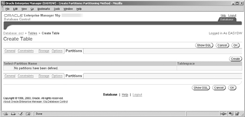
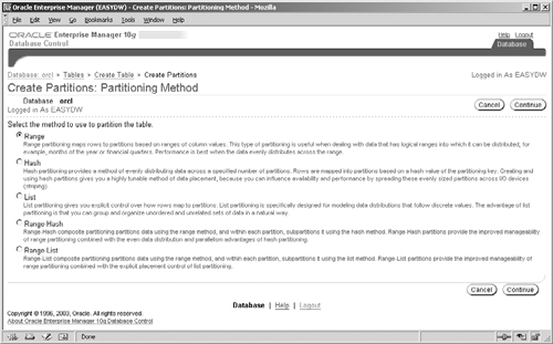
When you first get to this page, you will see a Create button, which, when clicked, will take you to the Create Partitions screen shown in Figure 4.6. Here you can choose the partitioning method: Range, Hash, List, Range-Hash, or Range-List. In our example, we have chosen range partitioning.

Figure 4.6. Choosing the Partitioning Method

The next step is to choose the partitioning column (or possibly multiple columns for range partitioning). You will be shown a list of all the table columns and a box for each, under the heading Order. For those columns that you want to include in the partitioning key, you must enter their desired position in the box. For instance, if we wanted to partition by PRODUCT_ID, TIME_KEY, we would put a 1 in the Order box for PRODUCT_ID and 2 for TIME_KEY. In Figure 4.7, we have chosen to partition by TIME_KEY.

Figure 4.7. Specifying the Partitioning Key

For range partitioning using a single column partition key of date or numeric type, this wizard provides a way to automatically generate the partition bounds. You need only to specify the desired number of partitions, the minimum value of the column, and the desired range of values in each partition. For instance, in Figure 4.8, we have specified that we would like five partitions with the earliest TIME_KEY value being 1/1/2003 and each partition containing one month of data. Later, you will be given a chance to edit the partition bounds and tablespaces; however, this is a very convenient starting point.

Figure 4.8. Automatically Generating Range Partition Bounds

The next screen (not shown here) asks you to pick tablespaces for the partitions. You can either specify a common tablespace for all partitions or a list of tablespaces, which will be used in a round-robin fashion for the partitions.

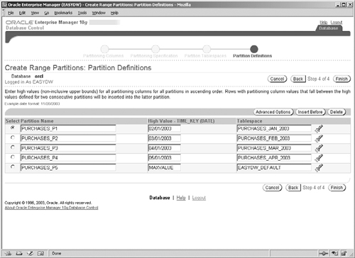
The final screen, shown in Figure 4.9, shows the automatically generated partitions. Now you can edit partition names, bounds, and tablespaces. You can also insert additional partitions or delete partitions.

Figure 4.9. Editing Partition Definitions

Further, for each partition, you can click the Advanced Options button, which will bring you to the screen shown in Figure 4.10. Here you can specify all the storage parameters and also indicate whether you would like to turn on data segment compression, which we discussed previously. You can also specify whether you would like to use the NOLOGGING option, which will turn off redo logging during maintenance operations on that partition; this can significantly improve performance. However, with the NOLOGGING option you can no longer recover the data after a database crash, so you must ensure that you have adequate backups of the data.

Figure 4.10. Specifying Advanced Storage Options for a Partition

If you chose any other partitioning method, the overall flow would be very similar to what we have seen, except that you will not be able to generate partitioning bounds automatically. You must enter the bounds manually in the final screen. For instance, Figure 4.11 shows a table using list partitioning.

Figure 4.11. List Partitioning

We mentioned earlier that partitioning simplifies data management in a data warehouse. This is because you can manipulate partitions in various ways to add, delete and reorganize data within the table more quickly than performing individual INSERT or DELETE statements. Some of the operations you can perform with partitions are as follows:

For composite partitions, similar operations are available at the subpartition level also. These operations are available using the ALTER TABLE SQL command. For example, to add a new partition to the PURCHASES table, you would issue the following SQL:

ALTER TABLE purchases ADD PARTITION purchases_jan2005
values less than (TO_DATE('01-JAN-2005', 'DD-MON-YYYY'));

Using combinations of partition maintenance operations, you can speed up loading new data and archiving old data in a data warehouse. We will discuss various techniques using partition maintenance operations in Chapter 11.

In this section, we have seen how use of partitioning provides great benefits in a warehouse by improving query performance, manageability, and availability of the data. Next we will discuss techniques for indexing a data warehouse and how partitioning can be applied to indexes.

B*tree indexes are hierarchical structures that allow a quick search for a row in a table having a particular value of the index keys. A B*tree index stores pointers to rows of the table using rowids, which uniquely identify the physical location of rows on disk. There are two varieties of B*tree indexes:

A unique index ensures that each row has a distinct value for its key—no duplicates are allowed. A unique index is automatically created when a PRIMARY KEY or UNIQUE constraint is enabled on a table. The following SQL statement creates a unique index on the TIME_KEY column of table TIME:

CREATE UNIQUE INDEX TIME_UK ON TIME(time_key);

B*tree indexes can also be nonunique. Nonunique indexes improve query performance when a small number of rows are associated with each column value. In the SQL statement for creating an index, if you do not specify the UNIQUE keyword, the index is considered nonunique.

When multiple columns are used together in the WHERE clause, you can build an index on that group of columns. Indexes made up of multiple columns are called composite, multikey, or concatenated indexes. For example, city and state are both needed to differentiate Portland, Maine, from Portland, Oregon. The column that is used most frequently by itself should be specified as the first column in the index. In the example, state should be the leading column, since we can anticipate queries on state alone or city and state used together.

Whenever a row is inserted, deleted, or when the key columns are updated, the index is automatically updated to reflect the change. A B*tree index is designed such that the time required to search any particular value in the index is nearly constant. This design is called a balanced index. As new index nodes are created, the B*tree is automatically rebalanced. Index maintenance therefore adds overhead to the DML statement.

A B*tree index is most useful when the index key has many distinct values, each leading to a few rows in the table. For instance, a primary key implies each value of the key corresponds to one row in a table. However, if the index key column has only a few distinct values, then each value would lead to retrieval of large numbers of rows in the table. This provides little, if any, performance benefit. For instance, consider the query: How many women who live in California buy tents? There are only two possible values for the column GENDER. Since not all records with the same gender value may be stored together, finding all the rows corresponding to women may result in a random scan of nearly all data blocks in the table. In this case, a full table scan may be more efficient. Also, for large tables, space requirements for B*tree indexes could become prohibitive.

Bitmapped indexes are designed to solve these problems and hence are more commonly used in a warehouse.

Bitmapped indexes are designed to answer queries involving columns with few distinct values but potentially large numbers of rows for each value. The number of distinct values of a column is known as its cardinality. Unlike B*tree indexes, which store pointers to rows of the tables using rowids, a bitmapped index stores a bitmap for each distinct value of a column.

The bitmap for each distinct value has as many bits as the number of rows in the table. The bit is set if the corresponding row has that value. Figure 4.12 shows a bitmapped index for the GENDER column (cardinality = 2, distinct values—M and F). Two bitmaps are created one for the value M and one for the value F. In the bitmap for M, all rows with male customers would have their bit set to 1 and all female customers would have their bit set to 0.

Row   Gender   Male Bitmap   Female Bitmap
1      M       1              0
2      F       0              1
3      M       1              0
4      M       1              0
5      M       1              0
6      F       0              1
7      M       1              0
8      M       1              0
9      F       0              1
10     M       1              0

Bitmapped indexes on two columns of a table can be combined efficiently using the AND and OR Boolean operators. This allows them to be used for queries involving multiple conditions on bitmapped columns of a table. This gives the benefit that you can answer a wide variety of queries with just a few single-column bitmapped indexes.

For instance, suppose we had a CUSTOMER table that contained the customer name, gender, and occupation (teacher, engineer, self-employed, housewife, doctor, etc.). We are looking at a new promotion targeted toward self-employed women and would like to find out the cities to target. This can be expressed as a query:

SELECT customer_id, city
FROM customer
WHERE gender = 'F' AND occupation = 'Self-Employed';

Figure 4.13 shows the bitmap for the occupation column.

Row   Occupation  Teacher    Engineer Self-Employed   Housewife
1     Teacher           1           0             0            0
2     Engineer          0           1             0            0
3     Teacher           1           0             0            0
4     Teacher           1           0             0            0
5     Engineer          0           1             0            0
6     Self-Employed     0           0             1            0
7     Self-Employed     0           0             1            0
8     Housewife         0           0             0            1
9     Engineer          0           1             0            0
10    Housewife         0           0             0            1

The gender bitmap defined in Figure 4.12 and the occupation bitmap defined in Figure 4.13 can be combined, as shown in Figure 4.14, to quickly determine the rows in the customer table that satisfy this query.

Row   Female   Self-Employed     Result
1         0                0          0
2         1                0          0
3         0                0          0
4         0                0          0
5         0                0          0
6         1                1          1  (Self-Employed Woman)
7         0                1          0
8         0                0          0
9         1                0          0
10        0                0          0

The SQL statement used to create the bitmapped index on the CUSTOMER.GENDER column is as follows:

CREATE BITMAP INDEX easydw.customer_gender_index
ON customer(gender) tablespace indx;

Bitmapped indexes are automatically compressed and therefore require much less space than a corresponding B*tree index. The space savings can be significant if the number of distinct values of the bitmap is small compared with the number of rows in the table.

The main disadvantage of bitmapped indexes is that they are expensive to maintain when the data in the table changes. This is because the bitmaps must be uncompressed, recompressed, and possibly rebuilt. Bitmapped index maintenance is optimized for the common case of loading new data into a warehouse via bulk insert. In this case, existing bitmaps do not need change and are simply extended to include the new rows. In Oracle Database 10g, enhancements have been done to improve the performance and space utilization of bitmapped indexes even when DML other than bulk loads is done to the tables.

Another difference between B*tree and bitmapped indexes is that if a B*tree index updates a row, it only locks that particular row; however, with bitmapped indexes, a large part of the bitmap may need to be locked. Thus, bitmapped indexes reduce the concurrency in the system, and so bitmapped indexes are not suited for systems with lots of concurrent update activity. High update activity is generally not a characteristic of data warehouses and hence bitmapped indexes are very common there.

A bitmapped join index is a bitmapped index that is created as the result of a join between a fact table and one or more dimension tables. To illustrate the concept of bitmapped join indexes, consider the following query, that asks the question: How much did women spend in our store?

SELECT sum(p.purchase_price)
FROM purchases p, customer c
WHERE p.customer_id = c.customer_id
      AND c.gender = 'F';

We could create a bitmapped index on the CUSTOMER.GENDER column, as discussed in the previous section, to find those customers who are women quickly. However, we would still need to compute the join between PURCHASES and CUSTOMERS to find the total purchases made by women.

Instead, if we take the answer to the join and then create a bitmap to identify rows corresponding to purchases made by men and women, we get a bitmapped join index. Figure 4.15 shows the answer to the join between PURCHASES and CUSTOMER table (only first 10 rows are shown).

Row   Customer_id  Gender  Purchase_price
1     AB123456          F          28.01
2     AB123457          F          28.01
3     AB123457          F          28.01
4     AB123457          F          28.01
5     AB123456          F          67.23
6     AB123457          F          67.23
7     AB123458          M          67.23
8     AB123459          M          67.23
9     AB123460          F          67.23
10    AB123461          M          50.71
...

The bitmapped join index has two bitmaps one for the value male and another for the value female, as shown in Figure 4.16. Each row in the bitmap corresponds to a single row in the PURCHASES table. Thus, we can immediately identify the rows for purchases made by women from the bitmap for value female.

Row   Gender     Male Bitmap        Female Bitmap
1     F          0                   1
2     F          0                   1
3     F          0                   1
4     F          0                   1
5     F          0                   1
6     F          0                   1
7     M          1                   0
8     M          1                   0
9     F          0                   1
10    M          1                   0
...

The bitmapped join index on PURCHASES, joined with CUSTOMER, is created using the following SQL statement. The joining tables and their join conditions are specified using the FROM and WHERE clauses, similar to those in a SELECT statement. The table on which the index is built is specified by the ON clause, as with any other index.

CREATE BITMAP INDEX easydw.purchase_cust_index
ON
purchases (customer.gender)
FROM purchases, customer
WHERE purchases.customer_id = customer.customer_id;

We can immediately note some differences between a bitmapped index and a bitmapped join index. While a bitmapped index is created on columns of a single table, a bitmapped join index is built on the fact table (PURCHASES), but the index columns are from dimension tables (CUSTOMER).

As with a bitmapped index, columns included in a bitmapped join index must be low-cardinality columns. For a bitmapped join index to make sense, the result of the join should have the same number of rows as the fact table on which it is created (in our example, the PURCHASES table). To ensure this, a unique constraint must be present on the dimension table column that joins it to the fact table (in our example, the CUSTOMER.CUSTOMER_ID column).

Bitmapped join indexes put some restrictions on concurrent DML activity on the tables involved in the index, but, again, this is not a major issue for data warehouse applications.

One of the common problems with indexes is that if the query involves a function on the indexed column, then the optimizer will not use the index. To solve this problem, B*tree and bitmapped indexes can be created to include expressions and functions involving table columns, instead of simple such as columns as the index key. Such indexes are known as function-based indexes. Function-based indexes are useful when your queries contain a predicate with a function, such as TO_UPPER() or TO_NUMBER(), or an expression such as PURCHASE_PRICE+SHIPPING_CHARGE. To be able to index a function, the function must be deterministic or, in other words, must return the same result every time it is called with the same arguments. For example, the built-in SQL function SYSDATE, which returns the current date, cannot be used, because it gives a different value every time it is invoked.

The following example shows a function-based index on the column PRODUCT_ID and the column CATEGORY, with the UPPER function applied to it to capitalize its contents.

CREATE INDEX prod_category_idx
ON product (product_id, UPPER(category));

The function that we use in our index can also be a user-defined PL/SQL function, provided that it has been tagged as DETERMINISTIC, as shown in the following example:

CREATE OR REPLACE FUNCTION TAX_RATE(state IN varchar2,
                                    country IN varchar2)
RETURN NUMBER DETERMINISTIC IS
BEGIN
 ...
END;
/

This function, TAX_RATE, can now be used in an index, as shown in the following example:

CREATE INDEX customer_tax_idx
ON customer (TAX_RATE(state, country));

When creating a bitmapped index with a function, just as with columns, you must ensure that the function has low cardinality or, in other words, a few possible output values; otherwise, a bitmapped index is not very useful. At the time of writing, bitmapped join indexes did not allow functions.

In the next section, we discuss how partitioning can be applied to indexes.

As with tables, B*tree and bitmapped indexes can also be partitioned. Oracle allows a lot of flexibility in how you can partition B*tree indexes. A B*tree index can be partitioned even if the underlying table is not. Conversely, you can define a nonpartitioned B*tree index on a partitioned table, or partition the index differently than the table. On the other hand, a bitmapped index must be partitioned in the same way as the underlying table.

Partitioned indexes can be of two types:

Global Indexes

A global index cannot be partitioned at all, or, if it is partitioned, it can have a completely partition key different from the table. In a partitioned global index, the keys in an index partition need not correspond to any specific table partition or subpartition. Global indexes can be partitioned using range or hash partitioning methods. However, a partitioned global index must have the partitioning key of the index as the leading column of the index key.

Hint

Any index that is not partitioned is automatically considered a global index.

Figure 4.17 shows a global index, PURCHASE_PRODUCT_INDEX, on the PURCHASES table. Here, the PURCHASES table is partitioned by TIME_KEY, but the index is partitioned by PRODUCT_ID. The leading column of the index is also PRODUCT_ID.

Figure 4.17. Global Index on Product, Partitioned by product_id

The SQL used to create this index is as follows:

CREATE INDEX easydw.purchase_product_index on purchases
 (product_id)
 GLOBAL
 partition by range (product_id)
 (partition sp1000 values less than ('SP1000') ,
  partition sp2000 values less than ('SP2000') ,
  partition other  values less than (maxvalue) );

Figure 4.17 shows why global indexes may not be very efficient for query processing. Since there is no correlation between the table and index partitions, accessing a specific value in a table may involve access to several or all of the index partitions. On the other hand, if you would like a unique index, which does not include the partitioning key of the table, you will have no choice but to use a global index.

Another reason why global indexes can be expensive is that when the data in an underlying table partition is moved or removed using a partition maintenance operation (see section 4.2.9), all partitions of a global index are affected, and the index must be completely rebuilt. The shortcomings of a global index are addressed by local indexes.

CREATE  INDEX easydw.purchase_time_index
 ON purchases (time_key, customer_id)
local
 (partition indexJan2003 tablespace purchases_jan2003_idx,
  partition indexFeb2003 tablespace purchases_feb2003_idx,
  partition indexMar2003 tablespace purchases_mar2003_idx );

Nonprefixed Local Indexes

Local indexes that do not include the partitioning key as the leading column of the index key are known as nonprefixed local indexes. Such indexes are useful when we would like to partition by one column for ease of maintenance but index on other columns for data retrieval. For instance, we may want our indexes and tables to be partitioned by TIME_KEY, so that it is easy to add a new month’s data and rebuild the index partition for that month. However, to get good performance for queries for sales by PRODUCT_ID, we need an index on PRODUCT_ID.

Figure 4.18. Prefixed Local Index on time_key

Figure 4.19 shows a local nonprefixed index on the PRODUCT_ID column of the PURCHASES table. The partitioning scheme is the same as that of the PURCHASES table (i.e., on the TIME_KEY column) however, there is a separate search tree on the PRODUCT_ID column, corresponding to each table partition.

Figure 4.19. Nonprefixed Local Index on Product, Partitioned by Month

The following example shows the SQL to create this local index:

CREATE BITMAP INDEX easydw.purchase_product_index
ON purchases  (product_id)
LOCAL
 (partition indexJan2003 tablespace purchases_jan2003_idx,
  partition indexFeb2003 tablespace purchases_feb2003_idx,
  partition indexMar2003 tablespace purchases_mar2003_idx);

Note the difference between the local nonprefixed index on PRODUCT_ID, shown in Figure 4.19, and the global index on PRODUCT_ID, shown in Figure 4.17. In the local nonprefixed index, there is a separate search tree for each table partition, and so, when searching for sales of some product—say Tents the optimizer is not able to perform partition elimination and must search for the data for all months. On the other hand, in the global index, there is one common search tree for all the table partitions. Thus, in this case, a global index can in fact provide better performance, because multiple index search trees do not need to be probed. However, when searching for Tents sold in January, the optimizer can indeed eliminate the February and March partitions of the index and so the local index will perform better.

An index improves performance of a query but is associated with two types of costs: First, it takes up disk space, and, second, it takes time to maintain when the underlying data changes.

Space requirements for indexes in a warehouse are often significantly larger than the space needed to store the data, especially for the fact table and particularly if the indexes are B*trees. Hence, you may want to keep indexing on the fact table to a minimum. Typically, you may have one or two concatenated B*tree indexes on the fact table; however, most of your indexes should be bitmapped indexes. Bitmapped indexes on the foreign-key columns on the fact table are often useful for star query transformation, as discussed later in Chapter 6. Bitmapped indexes also take up much less space than B*tree indexes and so should be preferred. On the other hand, dimension tables are much smaller compared with the fact table and could be indexed much more extensively. Any column of the dimension table that is frequently used in selections or is a level in a dimension object (to be described in Chapter 8) is a good candidate for indexing.

Typical warehouses have low update activity, other than when the warehouse data is refreshed, and usually you would have control over when and how the refresh is performed. Hence, a warehouse can have many more indexes than an OLTP system; however, you must ensure that they fit within the maintenance window you have for your data warehouse. When loading new data, it is often faster to drop indexes and rebuild them completely after the load is complete.

The maintenance window will also dictate whether you use partitioned indexes, which can be faster and easier to maintain.

The wizard to create indexes can also be found in the Administration section of Oracle Enterprise Manager. Figure 4.20 shows the first screen of the wizard, where you can create either a bitmapped or B*tree index. Once you have entered the table name, you can click the adjoining Populate Columns button to display a list of available columns. You can then indicate the columns you would like to include in the index by specifying their ordinal position in the index key. For example, in Figure 4.20 we are creating an index on (PRODUCT_ID, TIME_KEY) of the PURCHASES table. It is not possible to create a function-based index through this wizard at this time.

Figure 4.20. Creating an Index

Notice that in Figure 4.20 near the Tablespace box there is a button Estimate Index Size. If you click this button, Oracle will estimate the storage the index would occupy once created. For this computation to be done, you must have at least specified the index columns. However, if you have specified storage options, such as the tablespace name and the PCTFREE value, you will get a more accurate figure.

If you click on the Options tab in Figure 4.20, you will be able to set various index options, as shown in Figure 4.21. These options include whether to build the index in parallel, with the specified degree of parallelism and whether to do index key compression. You can indicate if the data for the index is already sorted, which will speed up creation of the index.

Figure 4.21. Setting Index Options

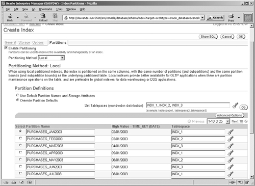
If you are creating a partitioned index, you can define the index partitions by clicking on the Partitions tab. You will get the screen shown in Figure 4.22, with the Enable Partitioning box unchecked. Once you check this box, you will be able to choose the partitioning method: Local, Global Range, or Global Hash. If you choose local, recall that the partition bounds are identical to that on the underlying table. You can, therefore, either use default partition names and tablespaces (which are same as for the table) or choose Override Partition Defaults to edit them, as shown in Figure 4.22.

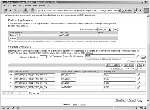
If you choose global partitioning, you will get the screen shown in Figure 4.23. You must first choose the partitioning key and specify the number of partitions. Once you have done this, click the Add button to get a list of partitions with default names. You can then specify the partition bounds (for range partitioning) and edit the partition names and the tablespaces to use.

Figure 4.22. Partitioning an Index

Figure 4.23. Global Partitioning

Once you have chosen all the options, you can click OK to create the index. The Show SQL button can be used to see the SQL statement for the index.

To create an IOT, you must specify the ORGANIZATION INDEX clause in the create table statement. When creating the index, you can specify the columns to include in the index using the INCLUDING clause. All other columns will be stored in the overflow segment. The following example shows the SQL to create an index-organized table:

CREATE TABLE      prodcat
(product_id       number,
 category        varchar2(10),
 description     CLOB,
 detailed_specs  BLOB,
 constraint pk_prodcat PRIMARY KEY(product_id)
)
ORGANIZATION INDEX
INCLUDING category
PCTTHRESHOLD 30
TABLESPACE prodcat_idx
STORAGE (INITIAL 8k NEXT 8k PCTINCREASE 10)
OVERFLOW
STORAGE
(INITIAL 16k NEXT 16k PCTINCREASE 10);

The INCLUDING clause indicates that all columns after CATEGORY—namely, DESCRIPTION and DETAILED_SPECS—should be placed in the overflow segment. Notice that there are two separate storage clauses: one for the index segment and one for the overflow segment. You can also specify a threshold value, known as PCTTHRESHOLD, which indicates the maximum percentage of an index block to use to store non-primary-key index columns. For each row, all columns that fit within the threshold will get stored in the index segment, and the remaining will go into the overflow segment. In this example, the PCTTHRESHOLD value has been set to 30 percent.

Note that if the PCTTHRESHOLD value is not large enough to hold the primary key, or if you have not specified an overflow segment and it is needed, you will get an error.

If you use Oracle Enterprise Manager to create your tables, one of the very first choices you will need to make is whether you would like to create a heap- or index-organized table, as shown in Figure 4.25.

With Oracle 9i and 10g, IOTs have been significantly enhanced and now support nearly all features that normal tables do. For example, you can partition an IOT with range, hash, and list partitioning. However, at this time, composite partitioning for an IOT is not supported. You can create B*tree and bitmapped indexes on an IOT. These indexes are known as secondary indexes and can be partitioned or nonpartitioned.

To create a bitmapped index on an IOT, the IOT must have a mapping table that maps logical rowids to physical ones. You can add a mapping table clause to the CREATE TABLE or add one later, as shown in the following examples:

-- create mapping table
ALTER TABLE prodcat MOVE MAPPING TABLE;

-- change mapping table storage options
ALTER TABLE prodcat MAPPING TABLE allocate extent (size 16k);

Figure 4.25. Choosing Table Organization—Heap versus Index

In a data warehouse, an IOT can be useful when you have dimension tables or lookup tables, such as product catalogs, where a small number of columns form a primary key and are used for querying, whereas other columns, such as product specifications or photos, are not frequently used and occupy, significant amount of space. To keep the index small, these non-key columns should be stored in the overflow segment of the index.

IOT organization for the fact table is not very common, because the fact table typically does not have a primary key. Another reason is that a fact table usually has several non-primary-key measure columns, which are frequently accessed, and therefore the space advantages of an IOT may not be realized. There are also a couple of other key differences between regular tables and IOTs, which make them somewhat unsuitable as fact tables. The primary key constraint on an IOT cannot be deferred or disabled. Checking validity of a constraint is a time-consuming operation, and, hence, when loading new data into the data warehouse, it is common practice to defer or disable all constraints and enable them only after the load is complete. This cannot be done if the fact table is an IOT, which can make the load process more expensive. Also, IOTs do not have physical rowids, which are necessary to use some refresh features of materialized views (see Chapter 7).

Oracle 9i, Release 2, introduced a technique for table compression known as data segment compression. In the Oracle database, data is stored in segments, each of which ultimately consists of data blocks: A data block can be thought of as the smallest unit of storage in the database, by default, 8K in size. Data segment compression compresses a table by identifying repeated values of data within each data block and places them in a lookup table at the beginning of the block. The data rows then point to the value in the lookup table. This can significantly reduce storage used when the data contains large repeating values, especially strings. It is especially useful for materialized views with aggregation, since the data values for the grouping columns are often repeated. Data segment compression can be done for a table or a partition of a table.

When a query is issued against a table compressed in this manner, Oracle will automatically uncompress the rows to return the result. Even though this may appear to be an additional overhead, it is not very significant and will be far outweighed by the I/O savings due to the reduced table size.

Table compression should be considered only if the table rows are not very likely to change. If new rows are added to a compressed table using a conventional INSERT statement, the new data is not compressed efficiently. Similarly, DELETE and UPDATE statements cannot maintain compression efficiently. However, if data is added using DIRECT PATH insert (using SQL Loader or an INSERT /*+APPEND */ statement), the new data is inserted into new blocks, which can be compressed. Hence, segment compression is well suited for data warehousing environments that do batch loads of data or for partitions that are mostly read-only.

To enable data segment compression you must specify the COMPRESS keyword when creating a tablespace, a table, or individual partitions of a range- or list-partitioned table. Note that data segment compression is not available for hash-partitioned tables, and, therefore, if reducing storage is your primary concern, you should consider an alternative scheme for partitioning. Data segment compression is also not available for index-organized tables.

The following example shows a range-partitioned table, PURCHASES, whose first three partitions are compressed. We have left the last one uncompressed, because more data may be added to this partition.

CREATE TABLE easydw.purchases
(product_id              varchar2(8),
 time_key               date,
 customer_id            varchar2(10),
 purchase_date          date,
 purchase_time           number(4,0),
 purchase_price          number(6,2),
 shipping_charge         number(5,2),
 today_special_offer     varchar2(1))
PARTITION by RANGE (time_key)
(
  partition purchases_jan2003
    values less than (TO_DATE('01-FEB-2003', 'DD-MON-YYYY'))
    tablespace purchases_jan2003 COMPRESS,
  partition purchases_feb2003
    values less than (TO_DATE('01-MAR-2003', 'DD-MON-YYYY'))
    tablespace purchases_feb2003 COMPRESS,
  partition purchases_mar2003
    values less than (TO_DATE('01-APR-2003', 'DD-MON-YYYY'))
    tablespace purchases_mar2003 COMPRESS,
  partition purchases_catchall
    values less than (MAXVALUE)
    tablespace purchases_maxvalue NOCOMPRESS );

If you are adding a partition with segment compression for the first time to a previously uncompressed partitioned table, you need to rebuild any bitmapped indexes on that table.

You may want to merge and compress partitions corresponding to older data, since they are not likely to change very much. This allows you to keep more data on-line. For instance, at the end of each month, you could compress the last month’s partition if it is unlikely to receive further updates. To change the compress attribute of a table you need to issue an ALTER TABLE MOVE command. For example, to compress the PURCHASE_CATCHALL partition of the PURCHASES table, you would issue:

ALTER TABLE purchases MOVE PARTITION purchases_catchall COMPRESS;

For B*tree indexes, Oracle performs key compression by storing only once the common prefix of index key values in an index block. Index key compression must be enabled using the COMPRESS keyword on the CREATE INDEX statement. Key compression is also possible for the index underlying an index-organized table.

For bitmapped indexes, the bitmap for each data value is automatically compressed by Oracle. For columns whose cardinality is much less than the number of rows in the table, the bitmaps tend to be dense (having a lot of 1s) and can be compressed greatly. Thus, a bitmapped index can occupy much less space than the corresponding B*tree index.