
Once the warehouse has been created and is populated with data, it is very important to ensure that it is correctly managed. The warehouse must be configured for optimal performance and availability. Disk, memory, and CPU resources must be managed effectively. In this chapter, we will describe some of the tasks involved in managing a data warehouse and provide advice on how to execute them.
We will make use of the various GUI tools provided in Oracle Enterprise Manager (OEM) to manage our database. There are alternative methods to this approach, but we are sure you will agree that using OEM makes managing the database considerably easier.
This chapter will first provide an introduction to OEM and then discuss various tasks, such as reorganizing the warehouse, gathering optimizer statistics, maintaining security, and monitoring space usage.
With Oracle Database 10g, Enterprise Manager changed significantly from the Java-based GUI tool to an easily accessible interface accessed via any browser on your wide area network. There are two named variants of Enterprise Manager: Database Control and Grid Control.
For managing an individual database and its ASM storage, EM Database Control is used, and this is the version that we are using predominantly in this chapter. EM Database Control is installed as standard with the database.
For managing multiple databases, application servers, and ASM storage components in your enterprise environment, Enterprise Manager Grid Control is used. EM Grid Control is installed from a separate installation CD.
EM Database Control provides a subset of the functionality that is present in EM Grid Control.
Therefore, from one lightweight browser you can manage your entire system, no matter where the components may be located. This is an extremely powerful capability, and you should remember that what we are describing here could be used not only for the data warehouse database but also for other Oracle databases—from versions 8.1.7 and above, Oracle Application Server 10g, and ASM storage on your network. In this section, we’ll take a look at some of the concepts and steps required to start using OEM.
Before we launch into a more detailed examination of the new Enterprise Manager, it is worth mentioning that we still have the old Java GUI EM console to handle certain aspects of managing our environment.
The Java EM Console is installed from the Client CD and still has the same familiar interface from its Oracle 9i version. With the Oracle Database 10g version, you will find that some of the tools have been removed to the browser version, such as the import and export wizards, backup wizard, the events and job scheduling tools, and the ability to create warehouse dimensions and cubes. For handling the following product areas you will still need to use the Console.
Streams
Advanced replication
Advanced queues
XML database
Spatial
None of these components is crucial to a data warehouse, so you can manage the warehouse environment exclusively using the browser-based interface.
EM Database Control, which we have been using so far, is for administering and managing an individual Oracle Database 10g at a time. As we have seen in previous chapters, you simply point your browser at the URL for the instance on a server that you wish to administer. The deployment is shown in Figure 11.1.
The URL for Database Control is shown in the following code, and the default port number is 5500. If you have multiple Oracle 10g databases on your server, then EM will be configured to use a different port number for each database. For example, the second database may be configured to use port 5501.
http://<server name>:port/em
The background tasks for the database console can be manually started and stopped from the operating system command line, using the Enterprise Manager command-line utility, emctl, as follows:
To start the console:
emctl start dbconsole
Or to stop the console:
emctl stop dbconsole
On a Windows system, Enterprise Manager uses a Windows service for operation. The Windows service name is OracleDBConsole<sid>, where <sid> is that for your database. For example, the service for the EASYDW database is OracleDBConsoleeasydw. The service will be configured during installation to start automatically at system startup.
However, if we want to be managing and administering a number of databases, and also other components such as Oracle Application Server 10g, then we need to use Enterprise Manager 10g Grid Control.
Enterprise Manager Grid Control is designed to run in a three-tier architecture.
The console, which is accessed using a browser, provides the graphical user interface on the client system.
The management service (OMS), which provides administrative functions, such as executing jobs and events, runs in the middle tier.
The management agents, which monitor the various targets on the servers, such as the database and ASM instances, start and stop them and gather performance data.
All information required to manage and administer the environment is stored in the OEM repository, which can be part of any Oracle database or in a separate Oracle database, which is used exclusively for Enterprise Manager. It is where the management service stores the information it needs to manage the network configuration, the events to monitor, jobs to run, and the administrator accounts.
The various components in EM Grid Control are shown in Figure 11.2. To manage a server and the different components deployed on it, you must have a management agent deployed. This is done as part of an installation separate from that for the database itself. In Figure 11.2, we have shown just two types of servers with agents deployed:
A server with two database instances and an ASM instance
A server with a Oracle Application Server 10g instance

Of course, via EM Grid Control you can administer as many servers and components as you have agents deployed
The Grid Control management service communicates with the agents via secure https. Your browser can communicate with the management service either via a nonsecure or a secure https connection. Considering the importance of your enterprise environment, we recommend you always use the secure https URL.
For EM Grid Control, the secure URL is different from the one for Database Control. For Grid Control, the default URL is:
https://<server name>:port/em
where the default port number is 7777.
To control the management service we again use the emctl command-line utility. To start the management service we execute the following from the operating system command line:
emctl start oms
The management agent must similarly be started and this is done as follows:
emctl start agent
We will continue looking at the new interface and features in the Enterprise Manager for now and have a further look at the extensions for Grid Control later in the chapter.
In Chapter 2, we have already touched upon how to access the EM login screen via the browser. When you logon to EM Database Control, you have the option of logging on as a normal user, an operator, or as SYSDBA. Each has different levels of privileges, and certain administration functions will not be available from all login types. For example, if you want to change the value of certain initialization parameters, such as shared_pool_size, then you will need to be logged on as a privileged SYSDBA account. We will assume that a DBA account is being used and point out any differences when we come across them.
When you have logged in, you are presented with the Home screen, shown in Figure 11.3, which provides you with a basic summary and status of your database operation. It is grouped into separate areas, and, if you scroll down further, you will see other areas, such as the Alerts section, where you can easily see if there are any critical alerts and notifications for your attention. We will look at alerts in more detail later in the chapter. The home page is also an active display. On the top right of the screen there is the View Data field, where you can switch from a manual refresh to a regular one every 60 seconds.
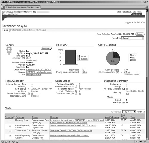
Even further down the screen (which isn’t shown), there is a section for-Job Activity and Critical Patch Advisories. We will look at jobs later in this chapter. The new patch advisory feature uses an Oracle Metalink connection, configured in OEM to determine whether or not any new patches have been released by Oracle and need to be installed on your system.
Enterprise Manager has four different home tab areas, which are accessed from the links at the top left of the screen. These are:
Home
Performance
Administration
Maintenance
The Home page is the initial login Home page with the summary information, where critical alerts and warnings are flagged for the administrator’s attention.
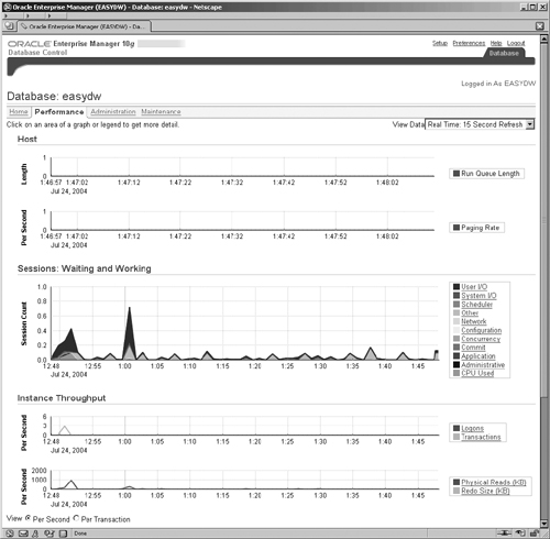
The Performance screen provides a new graphical user interface to show the performance and operation of the system and visually highlight problem areas. Various links by the graphs enable drill down, so that the administrator can analyze the system and focus in on any problem areas and even drill down to identify the SQL or other activity that is causing the problem. This is a very powerful new area and set of screens for assisting the administrator in problem identification and resolution.
We discussed various SQL tuning tools available from the Performance page in Chapter 10.
The Administration screen is the area that we have visited quite frequently during the course of this book. It is the main launch area to specific screens for administering the objects and other activities in the database. For example, we can administer the instance, monitor the memory usage, and change the initialization parameters from the Instance section. Or we can monitor and control the use of resources among our consumers in the database in the Resource Manager section.
From the work that we have done in the preceding chapters, you should now be quite comfortable with the look and feel of these administration screens, so, instead of reviewing each area, later in the chapter we will focus on some new areas, such as the Scheduler.
The Maintenance screen consists of three main areas for Utilities, Backup & Recovery, and Deployments. The Utilities section includes some areas that we have already talked about in Chapter 5, such as import and export and SQL*Loader. It also contains some other very useful features, such as Online Redefinition, which we will discuss later and Chapter 12 is dedicated to backup and recovery, and software upgrades is discussed in Chapter 17.
Finally, at the bottom of the screen, we have a small section on related links, which will take us to other important areas of Enterprise Manager. You will find the Related Links section is common to each of the four Home screens described previously.
Enterprise Manager Grid Control enables us to view the status of all of the components in our enterprise grid, including the host servers, the databases, the application servers, and the storage instances. EM enables us to drill down from the enterprise perspective to look at any aspect of the individual operation of these components. In this section, we will provide a brief overview of what we mean by this.
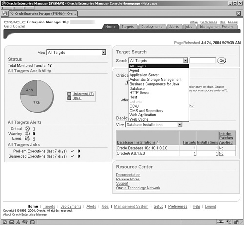
When we log on to EM Grid Control, our initial view and Home page is very different from what we are used to with EM Database Control. The EM Grid Control Home screen is shown in Figure 11.4.
Hint
Figure 11.4 shows the use of a drop-down list. Drop-down lists are a key feature used in Enterprise Manager screens for finding more options or actions that can be performed.
In Enterprise Manager, targets are components that you monitor or configure via Enterprise Manager. In the expanded drop-down list shown in Figure 11.4, we can see how the Grid Control interface enables us to view all component targets in our environment. The drop-down list demonstrates the comprehensive nature of what can be monitored and administered, such as databases, application servers, and ASM storage.
Notice that in Figure 11.4, we have a main tab menu at the top of the screen showing the following options:
Home
Targets
Deployments
Alerts
Jobs
Management System
For certain selections from this tab menu, a secondary menu, as shown in Figure 11.5, is displayed. The submenu for Targets contains entries for the different types of targets that can be administered; they are:
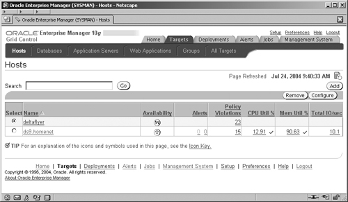
But to enable us to monitor and manage a target, Enterprise Manager must first know about it. To do this we must direct EM to discover the targets. This operation only needs to be performed once for a new server. Go to the top of the main Hosts screen, shown in Figure 11.5, select the Targets tab at the top, and then select Hosts from the submenu. Once the Management Agent on the new host has started talking to the Management Service, then your new host will appear in the list on the Hosts screen. Select the host on which you want EM to discover the targets and click on the Add button.
On the next screen (not shown) enter the name of the host and click the Continue button. This will start a task, which may take a few minutes to execute, where the EM management service is talking to the agent that is deployed on the new host. The agent examines its host environment and the targets that are deployed on it—for example, database instances or ASM instances—and communicates the findings back to the management service. These are then displayed in the Targets Discovered screen, shown in Figure 11.6.
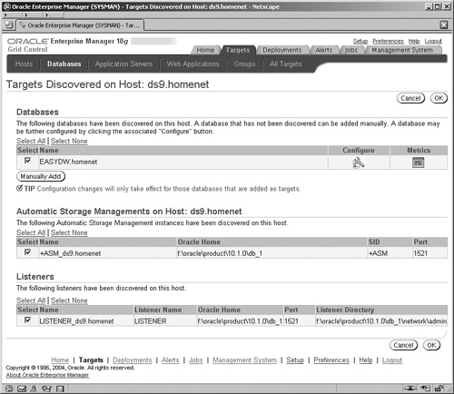
By clicking the OK button you accept the discovered targets and the metadata for these is written to the OMS repository. You are now able to access and drill down to manage these target components directly from the EM screens. For example, by selecting the Targets tab and Hosts subtab at the top of the screen, you will see the Hosts screen shown in Figure 11.5. Clicking on the name of a host in the list will navigate you to the host’s Home page for which there are four separate screens for the host: Home, Performance, Targets, and Configuration. By clicking on the Targets link, you will see a list of all of the targets on that host that are monitored by EM, as shown in Figure 11.7.
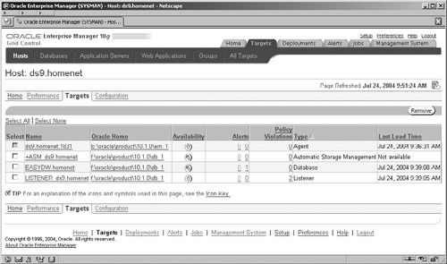
You can now click on the name of any of these targets to navigate to specific screens for the administration of that type of target. In Chapter 3, we have already seen some of the screens for administering an ASM instance. Alternatively, if the database name is clicked (which is third in our list), we navigate to the now very familiar EM Database Control Home pages for that database.
There is much, much more to Grid Control than we have space for in this chapter, so we have only provided a quick glimpse of its capabilities here. Grid Control is not just about the ability to monitor, diagnose, and control—though, as we have seen at the database level, it is a very important component—it is also about the ability to control resources across the grid.
To perform certain operations, an Enterprise Manager administrator account is required. An administrator account is a database account that has been enabled within Enterprise Manager to perform administration tasks. Database and normal Enterprise Manager accounts are not administrators by default. Enterprise Manager has two types of administrator accounts: regular administrators and super administrators, who have additional privileges.
A super administrator is created when Enterprise Manager is installed and configured. This is the SYSMAN account and, depending upon the password option you selected during database creation (see Figure 2.7), will either have your common password for key accounts or a specifically chosen one. Go to the Administration screen and select the Administrators link, which takes you to the Administrators Setup screen, shown in Figure 11.8 from where we can manage the administrators’ accounts.
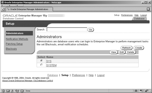
When we click the Create button, we can create a new administrator in the screen shown in Figure 11.9, where an existing database account can be selected and granted the privileges to be an administrator in Enterprise Manager. The Super Administrator is creating an account with the user name of EASYDW, for the DBA of the EASYDW data warehouse. Note that this is not a Super Administrator account, because we have not selected that option.

Earlier, we spoke of the issues surrounding managing multiple databases, and this applies equally to other targets in our grid, such as application servers and ASM instances. The purpose of a group is to allow you to logically associate the different targets in your environment to assist with the issues surrounding managing multiple targets. The Oracle grid in an enterprise environment can manage many different separate systems. For example:
Warehouse databases
Warehouse ASM instances
Application Servers
Source OLTP servers and databases
HR and payroll servers and databases
There are many other Oracle systems typically required for the running of the business that fall into this list.
In a large enterprise environment, we often require some way to group these together to help us better understand and appreciate the organization of the grid that we are administering. A group can consist of targets of the same type—for example, all databases—or it can consist of targets of different types, such as the database, ASM instances, and application servers for the warehouse. Some examples of ways that we may want to define the groups are:
A functional requirement—for example, all targets for the data warehouse
A geographical split for example, a group for the systems in the North-east United States and another for the systems in the United Kingdom.
An area of individual responsibility for example, the systems which are the responsibility of a particular administrator
You can only create and administer groups from EM Grid Control and not EM Database Control, because it is Grid Control that has the management framework for the administration of multiple targets.
To create a group, go to the Targets tab at the top of the Grid Control Home screen and select the Group subtab below it. The resulting screen (not shown) lists all of the groups that have been defined. To create a new group, choose the type of group and click the Go button. There are three types of groups that can be created:
Group, which can either be for mixed or for all the same type of targets.
Database Group, which is only for database targets
Host Group, which is only for host server targets
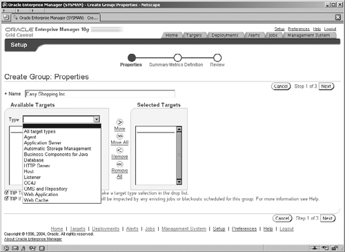
We have chosen to create a general group, which can contain targets of mixed types, the range of which you can see from the displayed drop-down list in Figure 11.10. On this screen you enter the name of the group, Easy Shopping Inc. When a target type is selected, the list is refreshed to display all available targets of that type, which you can then select and move to the Selected Targets list.
On the next screen of the wizard (not shown), you can define which metrics are to be collected and used for the group. This screen displays the metrics that are applicable to each type of target in the group. When the choice of metrics has been made, the minimum, maximum, and average of these for the targets are used for the alerts and warnings on the group’s Home page (see Figure 11.11).
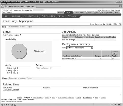
In Figure 11.11, we can see our group, called Easy Shopping Inc., which represents our warehouse. The screen is a summary display of key information about the hosts that make up our group. This is one of the powerful visual features of creating a group, because you can instantly look at the screen and see the state of your system. From this screen we may drill down and focus on different aspects of the various targets in the group by navigating to the Member Targets screen.
You may be saying to yourself: This is all very well, but what is the point? Later in the chapter, we will describe metrics, alerts, and warnings in more detail, and when these are combined with the group concept, you have a very powerful management environment.
Groups simplify the management of a complex environment by enabling the environment to be subdivided into logical groups, which serve a similar purpose. You can create as many groups as you like to assist with the management of your environment.
Data warehouses require a great deal of maintenance, because data is continually being loaded. You could write scripts to perform these tasks and remember to run them, or you could use the Scheduler in Enterprise Manager to automatically run your jobs at the designated time.
The new Scheduler facility in Oracle Database 10g provides the ability to define jobs that must be run in order to manage your data warehouse. These jobs can be placed in a library and scheduled automatically by EM to run at the specified time.
First, we need some simple definitions to help us understand the process:
The Program. This is the actual executable that we want to run.
The Job. This is metadata that defines how a program is to be run. It defines the argument values for the execution of the program.
The Schedule. This specifies when the job is executed. The schedule also defines whether or not, and how, the job repeats its execution.
Before we can create a job, we must first create a program that we want to run. A program can be a PL/SQL block, a stored procedure, or an operating system executable outside of the database. We will base our example on a small program to collect schema statistics. As we have seen in the previous chapters, the ability of the database optimizer to select the best access plan to get the data to answer the queries depends on statistics having been collected on our schema objects.
We will now create a program that gathers the statistics for a schema and for this we will use a simple PL/SQL stored procedure, which takes the schema name as its single parameter and calls a standard procedure, called GATHER_SCHEMA_STATS, in the package DBMS_STATS.
CREATE OR REPLACE PROCEDURE gather_schema_stats
   (schema_name IN VARCHAR2)
AS
BEGIN
  dbms_stats.gather_schema_stats(schema_name);
END;
/
To create a program, click the Programs link under the Scheduler section on the Administration screen and you will get a screen that contains a list of programs. Click the Create button on the right to get to the Create Program screen shown, in Figure 11.12, where we can define our program. Name your program and make sure that it is owned by EASYDW and that it is enabled. For our example, we have decided to use a naming convention with a _P suffix for the programs and _J suffix for the jobs. Make sure that you have clicked the Yes radio button so that the program is enabled.
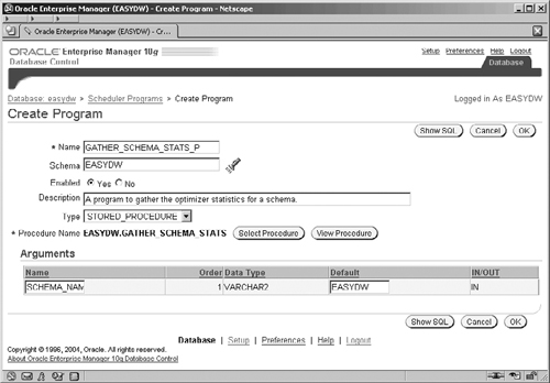
Now you have to specify the type of the program; in this example we are going to create one for a stored procedure. When you click on the Type box to select STORED_PROCEDURE, the screen layout will change to the screen shown and will contain extra fields that are specific to that program type. If the default procedure name shown isn’t the one for our stored procedure, then click the Select Procedure button. This will display a new screen (not shown), which enables you to select the GATHER_SCHEMA_STATS procedure in the EASYDW schema.
We will create our program as a stored procedure in order to demonstrate how the arguments work. In Figure 11.12, you can see that the single argument for our stored procedure has been displayed. At this point, we have the opportunity to provide a default value for the argument, which will be used if the program is invoked without any value at all. Enter EASYDW into the Default field.
Our program is ready to be created, and, if you click on the Show SQL button, you will see the screen shown in Figure 11.13, which Enterprise Manager is going to execute. This involves three calls to procedures in the DBMS_SCHEDULER package to create metadata about the program and the arguments and then to enable the program.
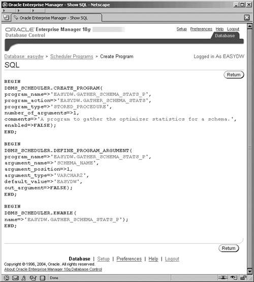
Click Return to go back to the Create Program screen and then OK to create the program.
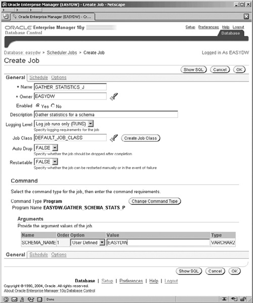
Now that we have created the program, we need to define the job that will execute it. In the Administration screen in the Scheduler section, click on Jobs to get to the Scheduler Jobs screen and then click the Create button to see the Create Jobs screen, shown in Figure 11.14.

In the same fashion as when we created the program, the Job screen defaults to fields for the command that are relevant to a PL/SQL block. Changing the command type will refresh the screen with fields appropriate to that type. In our example to gather schema statistics, we could have entered the call to the DBMS_STATS package directly into the PL/SQL block in this screen. However, this wouldn’t have helped demonstrate how programs and arguments are used by the Scheduler, which is why we are using a program.
Once you have completed the Name, Owner, and Description fields, click on the Change Command Type button and you will see the small screen shown in Figure 11.15 for selecting the program to be associated with this job.
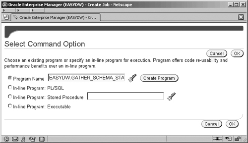
Select the Program Name radio button and the program that we just created and click OK. Figure 11.16 shows that the Command section now reflects our program with its single argument. If we fill in the Value field with EASYDW, then, whenever this job is run, it will gather statistics for the EASYDW schema.
There are two other screen tabs associated with creating a job. The first is to specify the schedule that is used for executing the job. Click on the Schedule link. The resulting screen, similar to that shown in Figure 11.17, enables us to specify whether or not the job should reexecute on a repeating basis and if so, when it repeats. Assuming that our warehouse will be refreshed every night, we would want the optimizer statistics to be collected daily at the end of that refresh task, just before the warehouse starts to be used for the business day. Click on the Repeat field and select By Days, and the resulting screen will be similar to that shown in Figure 11.17.
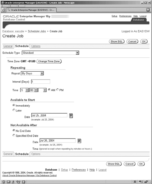
In Figure 11.17, there are four different ways to define the schedule for our new job, specified by the Schedule Type field.
Standard, where you can create a specific schedule, as shown in Figure 11.17.
Use Predefined Schedule, where the job uses a predefined and stored schedule. With this type, the stored schedule name is simply selected for use.
Standard, using PL/SQL for repeated intervals where a PL/SQL expression (e.g., “SYSDATE + 1” is the Enterprise Manager suggestion) is used to define the repeat interval.
Use Predefined Window, where a predefined window of operation can be used as a schedule. A job starts when the window opens and can be forced to stop when the window closes.
The remaining schedule fields on the screen change to be appropriate to the schedule type selected. We are using the standard schedule type. Similarly, the fields required to define the repeat schedule will change and be appropriate to the Repeat field value that is selected. The Available to Start and Not Available After parameters enable us to specify the boundaries within which our repeating schedule will operate. There is actually a lot of sophistication in how the schedule may be defined via this screen.
The definition of our job is almost complete. Clicking the Options link enables some more controls on the job execution, such as job priority, to be set, as shown in Figure 11.18.
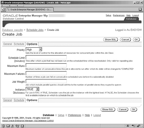
We don’t really need to set any of these for our job, though we should possibly consider setting the Priority. This defaults to Medium, but we may want to consider a higher priority to ensure that our statistics gathering completes, so we have raised its priority slightly to High. Clicking OK will create our job and return us to the Scheduler Jobs screen, where we can see our new job listed, as shown in Figure 11.19.
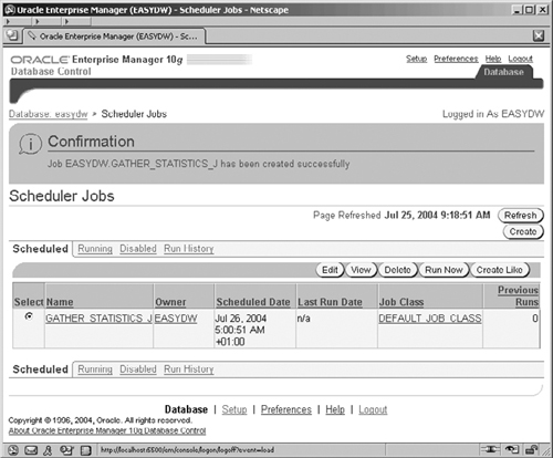
From this screen there are a number of links for tabs to display the jobs we have:
Scheduled
Currently executing
Marked as disabled
Already executed
We can use these lists to manage, edit, and monitor our jobs. For example, if we now wanted to disable the job that we have just created, we would click on its name, GATHER_STATISTICS, in the Name field in the Scheduled list and change the Enabled flag. Once the screens are refreshed, the job will have disappeared from the Scheduled list and appeared in the Disabled list. In a similar fashion, those jobs in the Run History list can be drilled into to examine their execution status and their results.
Distinct from the new Oracle Database 10g Scheduler jobs and programs that we’ve just discussed, there is another EM Job screen, which can be accessed by following the Jobs link in the Related Links section at the bottom of the four main Home pages.
The Job Activity screen shown in Figure 11.20 enables information about all EM jobs and current and previous executions to be searched for and examined. At the bottom of the screen, you can follow the link to the Job Library. The title of Jobs is used for both these EM Job screens and those for the new Oracle Database 10g Scheduler section, but these are actually two separate areas. You will notice that different jobs submitted by different parts of EM will utilize either these EM Job screens or the new Oracle Database 10g Scheduler job screens. For example, backup jobs will be listed in the Results section of this EM Job Activity screen; however, the new Segment Advisor jobs will be listed in the Run History list of the Scheduler Jobs screen.
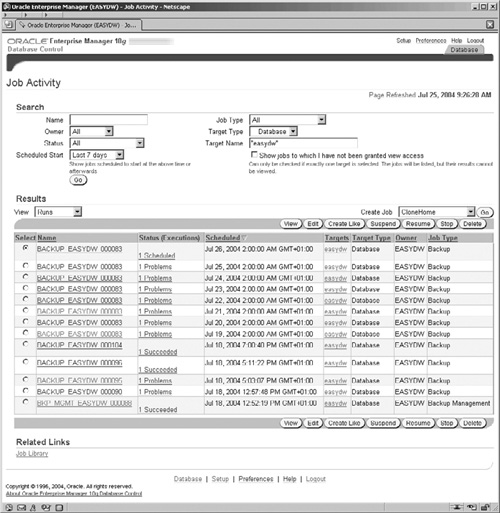
Figure 11.20 shows the Job Activity screen. By clicking on the job Name field in the Results section, the jobs can be drilled into. This will display new screens (not shown) containing information on the job’s execution, its individual steps, and the output logs from these steps—with further information on any error that may have occurred. For example, the backup jobs listed in Figure 11.20 show a problem that was caused by lack of space in the disk area where the backups were being written to.
To create a job, select the type of job that you want to create from the Create Job field on the right and click Go. The screen shown in Figure 11.21 will appear, which is where you describe the details for this job. In this example, we are again creating the job to collect the EASYDW schema statistics. First, we name the job and state upon which database it is to be performed. We can also define the accounts and passwords required for the job’s execution on both the server and the database, if necessary. Enterprise Manager has stored preferred credentials for our current login account, and this section allows us to override these defaults should we need to.

Although this example features a database task, other options are available from the drop-down list on destination type.
All jobs may be kept in the job library for reuse. Therefore, if you wish to retain the job, now is a good time to click on the button at the top of the screen to Save to Library.
The jobs form a library for reuse and can also be used by other user accounts. It is easy to see that a sophisticated suite of reusable components can be created. The other links on this page enable the job to be scheduled, and the Access link displays a screen where access to the new job can be granted to other administrators.
The examples in this section have shown a database operation and job. Alternatively, a job could be an operating system task that needs to be performed for managing the warehouse, such as ensuring that files are copied from one system to another prior to loading the warehouse.
The number of jobs that we can submit by both of the job mechanisms described in this chapter is quite extensive, and, once they are defined and as long as we are backing up our database, we have a comprehensive set of tasks that is safe and that can never be lost.
Oracle Database 10g introduces new tools for monitoring the performance of your data warehouse, diagnosing and providing recommendations for correcting any problems. The new components associated with this are the Automatic Workload Repository (AWR) and the Automatic Database Diagnostic Monitor (ADDM).
A database administrator may be barraged daily with questions about the performance of the warehouse. How do we make this SQL run faster? What is the problem? Where is the bottleneck? What do I look at to solve this one? These may be questions that your users have asked or they may be ones that you have asked yourself when something executes and grinds the database to a halt. The examination of what is happening on the database and where to look for information to resolve it comes from experience and knowledge. Similarly, the ability to know how to correct the problem without disrupting other aspects of the system often requires a knowledgeable Oracle person. On many occasions, solving one issue just uncovers another or can cause a problem elsewhere if care is not taken. Hence, the task of problem diagnosis and resolution can be a time-consuming and iterative process, which can take up quite a bit of a DBA’s time.
With the new AWR and ADDM components, Oracle Database 10g is addressing the perennial problem of assisting with the collection of the myriad data about the operation of the database and the analysis of this data to identify problem areas. AWR collects and stores the statistics and ADDM uses them to diagnose problems with the database performance. Oracle Database 10g is also providing new options and EM performance screens to increase the administrator’s ability to focus on the causes, and then EM assists with the correction and deployment of the solution.
The Automatic Workload Repository is a repository of the statistics and information about the operation of the Oracle Database 10g. To be able to understand what is happening as the database operates is a prerequisite to being able to analyze and resolve any problems that may occur; in order to be able to understand something, we must first have information about it. AWR is the repository of the information that enables us to understand the database operation. The statistics gathered are an enhanced superset of those used by Statspack in prior versions of the database. AWR is used by a number of other components in the database, such as the EM Performance screens and ADDM (which is discussed in the next section).
By default, every 30 minutes AWR collects detailed performance statistics and derived metrics on the operation of the database and stores these in the database. These are known as snapshots. The operation of AWR is designed and optimized to be an integral part of the database and not an operation that sits on top of it utilizing resources. Consequently, this integral aspect of the design and optimization minimizes the impact on the database operation and performance.
AWR is configurable and there are a number of parameters that control its operation. For example, the 30-minute collection frequency, which we have already mentioned, can be adjusted, as can the default seven days used to purge old snapshots. The AWR screens can be accessed by going to the Administration screen and clicking on the Automatic Workload Repository link in the Workload section. The resulting AWR screen, shown in Figure 11.22, enables you to view the general information about the AWR, such as the retention period and frequency that the snapshot is taken.
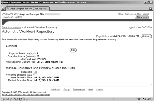
By clicking on the snapshot id number, the Snapshots page is displayed, where you can further control and manage snapshots. For example, you can use the snapshots to create a SQL Tuning Set (as described in Chapter 10) or create a set of preserved snapshots for future reference to use as the basis of a baseline for other metrics operations.
By clicking the Edit button on the AWR screen, the Edit Settings screen (not shown) is displayed, where you can adjust the retention period for the snapshots and the frequency with which they are taken—or even turn the snapshots off all together.
AWR and the comprehensive nature of the statistics that are collected underpin both the monitoring features of the EM performance screens (which are accessed from the Performance Home page) and the diagnostic capability that is possible with ADDM, which we will look at next.
ADDM is Oracle’s “expert DBA in a box.” It is a diagnostic engine that runs after every snapshot collection and analyzes the collected data to identify possible problems and recommend corrective actions. Principally, ADDM focuses on potential problem areas that are consuming a lot of database time and resources. It drills down to identify the underlying cause and creates a recommendation, with an estimate of the associated benefit.
First, we need to define the range of snapshots that we want ADDM to analyze. To launch ADDM, start at Advisor Central and in the list of Advisors click on ADDM. The resulting screen (not shown) enables you to specify the start and end snapshots and then create an ADDM task to analyze these snapshots.
To define the snapshot range, click on the Period Start Time radio button and then on one of the little camera icons under the graph. This specifies the start of your snapshot range. Then click on the Period End Time radio button and click on a camera icon for a later snapshot time. When you click the OK button, an ADDM task is created and executed. This task analyzes the data in AWR between your start and end points and provides you with a list of performance findings, as shown in Figure 11.23.
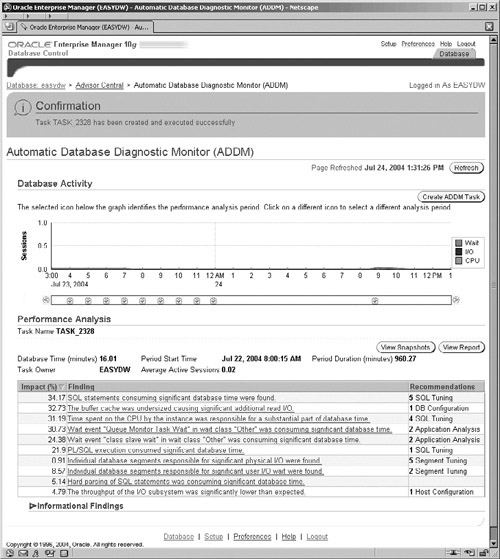
The Performance Analysis section, as shown in Figure 11.23, displays a list of the ADDM findings based on the snapshots that you specified. The ADDM findings are prioritized by the estimated impact on the system, as shown by the Impact (%) column on the left. Due to the different sets of metrics that ADDM analyzes, it also categorizes the findings, as shown by the Recommendation column on the right. For example, in the analysis findings we have shown in Figure 11.23, the highest impact is one involving potentially badly performing SQL. In the second finding, ADDM has discovered that the buffer cache is undersized and that the database configuration should be adjusted.
Note the two buttons on the right-hand side, which will enable you to view the information on the individual snapshots and also generate a very detailed HTML report of the finding.
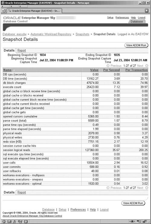
In Figure 11.24, you can see the result from clicking on the View Snapshots button in Figure 11.23, which contains details of the snapshots involved. By clicking on the Report link, you generate the comprehensive and user friendly HTML report.
From the list of the ADDM findings shown in in Figure 11.23, you can click on the Finding links for one of the findings categories that are displayed, and this takes you to other screens, which enable further drilling—even right down to the piece of nonperforming SQL or other cause of a problem. For example, by drilling down on a SQL statement that ADDM has identified, you get to the SQL Details screen (not shown), where there are different sections to enable you to examine more thoroughly the cause of the problem. These areas are:
From any of these four screens, you can then invoke the SQL Tuning Advisor (described in Chapter 10) to provide recommendations on how to correct the SQL.
This ability to drill down from the general to the specific is an approach adopted in many places within Enterprise Manager in order to facilitate the identification of a problem. For example, the graphs on the main Performance Home page, shown in Figure 11.25, operate in a similar fashion and use the historical snapshot data. The approach here is that the graphs display a larger block of color to indicate a possible problem area. You can then drill down using the links on the right-hand side to further identify the causes of the problems.
We have only touched upon the power of the new EM interface in order to demonstrate the functionality and importance of ADDM and AWR. These new features provide a very comprehensive set of monitoring and recommendation technologies, which appear in many aspects of the database operation and the management approach by EM. To assist with the normal day-to-day tasks in administering the warehouse, it will pay significant dividends for the DBA to explore and get a good understanding of these new features.
One of the problems for anyone managing a database is knowing when certain events occur. For example, suppose a tablespace fills up and has no free space remaining. Wouldn’t you like to know immediately that it has happened rather than wait for the calls from your users, who are complaining that the system is no longer available?
An alert is a notification that occurs when a metric, about which you have instructed the database to collect information, goes above a threshold target that you have set. Within Enterprise Manager, there are many alerts that are defined as standard and you see an example of these every time you log into Enterprise Manager in the Alerts section of the Home page. But you can also define your own alerts, which will allow you to monitor custom aspects of your data warehouse and be notified when certain events occur.
To manage these metrics, thresholds, and alerts, click on the Manage Metrics link in the Related Links section and you will get the screen shown in Figure 11.26. This screen lists the standard precreated metrics, as well as the custom ones, the thresholds that will trigger an alert, and the operator that defines the boundary criteria for the threshold. For example, the first metric in the list in Figure 11.26 is Archive Area Used, which is monitoring the disk space used by the archived redo logs; when it exceeds the 80 percent threshold, an alert is issued. When this occurs, you will see this alert on the Home page when you logon to Enterprise Manager.
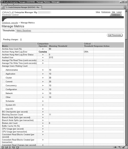
The thresholds and actions can be adjusted by clicking the Edit Threshold button, where a screen very similar to the one shown in Figure 11.27 is displayed, but this time the fields Warning Threshold, Critical Threshold, and Response Action are editable.
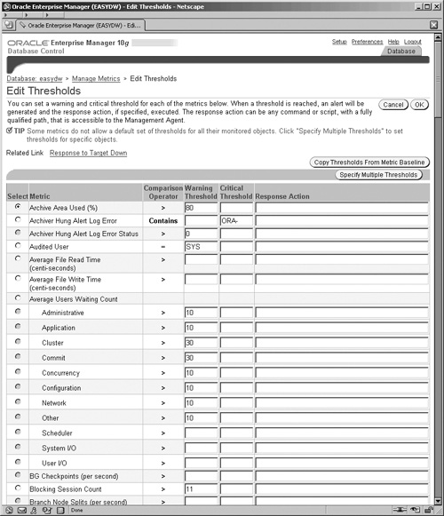
The Response Action field can be any operating system command, which includes calling custom programs and scripts. It is executed by the Management Agent running on the server, and this field is one of those that only superuser administrators can edit.
We can also define our own metrics on which a threshold can be based. On the Administration screen in the Related Links area, click on the User-Defined Metrics link at the bottom and then click the Create button to go to the Create User-Defined Metric screen, shown in Figure 11.28.

In the screen in Figure 11.28, we need to be able to express our metric in terms of either a SQL statement or a call to a function. To execute this code, we will also need to provide a database account name and password. In our example, we are using some SQL to read the database data dictionary to test if there are any materialized views that have the status NEEDS_COMPILE with a refresh date more than two days old. You can then specify the warning and critical conditions and the action to be performed. Our example will raise a warning if the OLD_AND_STALE value is returned from executing the SQL.
A useful feature here is the field in the Thresholds section to specify the number of consecutive times that the warning or critical threshold may be met prior to an alert being issued. This provides some control over temporary or transitory occurrences, which you may not want to be alerted about, but enables persistent ones to be flagged.
Here we have just scratched the surface of what is possible with metrics and thresholds. Much of the power of these features underpins the strength of the new monitoring and alert capability in Oracle Database 10g and is enhanced by the capability to customize for your own environment. Hopefully, this introduction will encourage you to investigate this area further and implement it as part of your data warehouse management procedures.
Reorganizing a database, irrespective of whether it is a data warehouse or a database used for transaction processing–style systems, is not a task to be undertaken lightly. Unfortunately, in a data warehouse, the time required to reorganize can become a serious issue, due to the high data volumes involved. Therefore, it shouldn’t be necessary to reorganize the database entirely, but minor changes may be necessary.
Reorganizations can occur for a variety of reasons, such as:
The business needs change
A regular archiving of data
The government changes the rules
Changes are required to the database design
Improve performance
The characteristics of the data were not as predicted
The integration of another company’s computer system following an acquisition
A change in the business requirements from the system is almost impossible to predict, and one solution to the problem may be to create a data mart rather than restructure the entire data warehouse.
The most probable reasons that we will need to reorganize are to improve performance, database changes, and archiving. Changing the physical implementation of the tables can certainly make a significant difference to the performance. Changing a table to be partitioned is a good example, but there may be more subtle changes, such as changing a column data type, which could also be required.
Careful reviewing of the database design and physical implementation can help overcome the need for later changes to the design and schema. If necessary, asking for an external review by an experienced data warehouse designer can be a good mechanism to identify potential problems as early as possible. One of the problems with data warehouses is that what may seem a good design at the outset may prove unsuitable in the long term, due to the large volumes of data involved. Therefore, try to minimize the likelihood of this occurring by using techniques such as partitioning.
Some reorganization may be planned. If you want to keep your data warehouse somewhat constant in size and not let it grow indefinitely, you may decide to keep only a few years of data. When new data is added, old data is archived and removed. This is called a rolling window operation and is discussed later in the book. The two major types of reorganization used in a data warehouse are partition operations and on-line reorganization, which we will look at in the next sections.
Some of the structural changes required by the data warehouse can be achieved by using partition operations. In this section, we will look at some of the most common partition maintenance operations, including the following:
Adding and dropping partitions
Exchanging a partition
Splitting and merging partitions
Coalescing a partition
Truncating a partition
Moving a partition
We will provide the full examples using SQL and also present the EM screens where the operation can also be performed. Where these are multiple-step operations, we will only demonstrate one of the steps in EM.
These operations are performed from the Edit Table screen EM following the Partitions link. When a partition has been chosen, a selection is made from the Actions box, which contains a list of the operations that can be performed on the partition when the Go button is clicked.
When the warehouse is first created, there may be little or no historic data with which to populate it. Therefore, for the first 18 to 24 months, new data continues to be added every month until the required system limits are met. Then, when the data warehouse is full, every month the old data is backed up and removed to make room for new data. Without partitions, the operation to delete the old data would have to scan all of the large fact tables to identify and delete the records, which is very time consuming. The faster alternative to this problem is to drop the partition containing the old data and create a new partition for the new data, as shown in Figure 11.29.
This technique is applicable only if the data is partitioned on a date or on a partition key that infers a date (i.e., that is time sequential, such as an absolute month number, for example, 200412 for December 2004). Therefore, if you decide upon another partitioning scheme, such as a code, this type of maintenance operation would not be possible. For example, it would be impossible to use with a hash partitioning mechanism, because you have no control over which partition Oracle will place the records into.
The SQL commands to perform the tasks are as follows. First, the old partition containing the data for sales for the month of January 2000 is dropped.
ALTER TABLE easydw.purchases
     DROP PARTITION purchases_jan00;
Next, the new partition for the data for sales for the month of December 2004 is created. The first step is to create the tablespace where the data will reside.
CREATE TABLESPACE purchases_dec04
DATFILE 'C:ORACLEPRODUCT10.1.0ORADATAEASYDWPURCHASESdec2004.f'
   SIZE 5m REUSE AUTOEXTEND  ON DEFAULT STORAGE
   (INITIAL 16k   NEXT 16k
    PCTINCREASE 0 MAXEXTENTS UNLIMITED);
The next step is to alter the table definition to create the new partition for December 2004 data in the new PURCHASES_DEC2004 tablespace.
ALTER TABLE easydw.purchases
     ADD PARTITION purchases_dec2004
       VALUES LESS THAN (TO_DATE('01-01-2005',
                                 'DD-MM-YYYY'))
       PCTFREE 0 PCTUSED 99
       STORAGE (INITIAL 64k NEXT 16k PCTINCREASE 0)
       TABLESPACE purchases_dec2004 ;
Of course, with this mechanism we had to drop the old tablespace in which the PURCHASES_JAN00 resided; otherwise, we would eventually end up with a collection of empty tablespaces that are not being used.
A slight variation of this technique is one where our tablespace names do not reflect the contents of the data they are holding. In Figure 11.30, we have named our partitions 1 through 60—instead of calling them after the data they hold, such as PURCHASES_JAN00. By using this approach, the tablespaces can then be reused. As we drop the old partition, it frees up the tablespace and then we simply reuse it to contain the new partition, as shown in Figure 11.30.
After a new partition is added to a table, data already can be loaded into it. Various techniques to load data were described in Chapter 5. If the data is in a table in the database, the fastest way to move the data into the new partition is by using exchange partition. This is used to move data from a non-partitioned table into a partition of a partitioned table. Exchange partition can also be used to convert a partition into a nonpartitioned table or between various types of partitioned tables. The following example shows moving the data from the DEC_ORDERS table into the PURCHASES_DEC2004 partition of the EASYDW.PURCHASES table.
ALTER TABLE easydw.purchases
   EXCHANGE PARTITION purchases_dec2004
   WITH TABLE dec_orders;
Most of the partition operations that we are going to look at in this chapter can be performed from Enterprise Manager by editing a partitioned table. From the Administration screen go to the Schema section and click on the Tables link. Select the PURCHASES table, and click on the Edit button to navigate to the Edit Table screen, and click on the Partitions link. This screen will show you a list of the partitions in the PURCHASES table. The Actions pick list on the right-hand side contains the list of operations that can be performed on a partition. Select Exchange from this list, click the Go button, and the screen shown in Figure 11.31 appears.
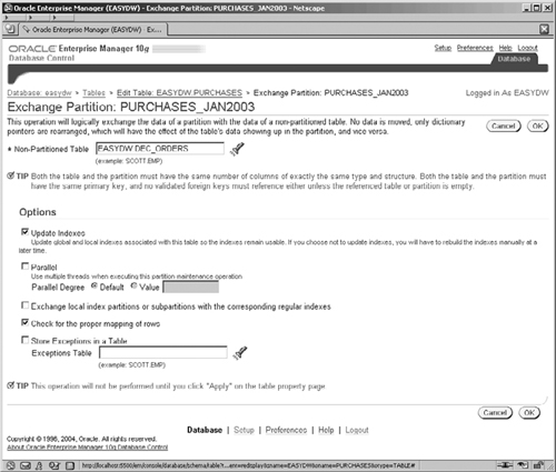
Select the nonpartitioned table that you want to exchange with the selected partition. In our example, the table is DEC_ORDERS but it only contains records for December 2004.
The reason that this operation is very quick is because no data movement is actually involved; Oracle is simply exchanging the metadata about the objects within the data dictionary. So the table’s metadata is redefined to be that of the partition of the PURCHASES table and the partition’s metadata is redefined to be that of the DEC_ORDERS table.
Partitions can be merged, either by merging into a wholly new partition or into an existing partition.
One technique often used by designers is to keep the first six months of data in monthly partitions, and then after that, store the data in quarterly partitions. By using the MERGE PARTITION option, the data can be easily moved to the new partition, as shown in the following code.
If we wanted to combine the data for April through July 2004 into a partition for the second quarter, we could merge the partitions. First, a new tablespace is created to store the Q2 purchases.
CREATE TABLESPACE purchases_q2_2004
   DATAFILE
'C:ORACLEPRODUCT10.1.0ORADATAEASYDWPURCHASESQ22004.f'
       SIZE 5M
       REUSE AUTOEXTEND ON
       DEFAULT STORAGE
          (INITIAL 64K NEXT 64K
           PCTINCREASE 0 MAXEXTENTS UNLIMITED);
In our example, there are three partitions that have to be merged, but the MERGE PARTITION command only allows us to merge two partitions at a time. Since only adjacent partitions can be merged, we will begin with merging May and June and then the resultant partition with April. If a table is partitioned by range, only adjacent partitions can be merged. Therefore, we can merge April and May or May and June but cannot merge April and June.
The new partition inherits the upper bound of the two merged partitions. Therefore, the two partitions with the highest ranges need to be merged first (May and June), into the Q2 partition. The following example merges the May and June partitions and stores them in the newly created tablespace called PURCHASES_Q2_2004. The PURCHASES_Q22004 partition is automatically added to the PURCHASES table.
ALTER TABLE purchases
        MERGE PARTITIONS purchases_may2004,purchases_jun2004
        INTO PARTITION purchases_q22004
        TABLESPACE purchases_q2_2004 ;
Next, the partition with the lowest range, PURCHASES_APR2004, is merged into the PURCHASES_Q22004 partition, as follows:
ALTER TABLE purchases
MERGE PARTITIONS purchases_apr2004,
purchases_q22004
INTO PARTITION purchases_q22004
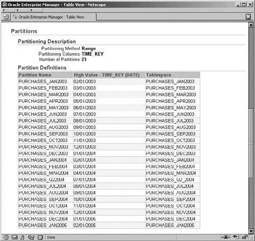
TABLESPACE purchases_q2_2004 ;After this operation, the PURCHASES table contains one partition, shown in Figure 11.32, which is showing the partitions section of the View Table screen for PURCHASES. Upon completion of the merge operation, the old partitions are automatically dropped from the PURCHASES table. The high value for the new PURCHASES_Q22004 partition is July 01, 2004.
This operation can also be performed by Enterprise Manager. On the Edit Table, Partitions screen, select the PURCHASES_MAY2004 partition, select the Merge action, click the Go button, and you are then presented with the screen shown in Figure 11.33, where you select the other partition with which you wish to merge.
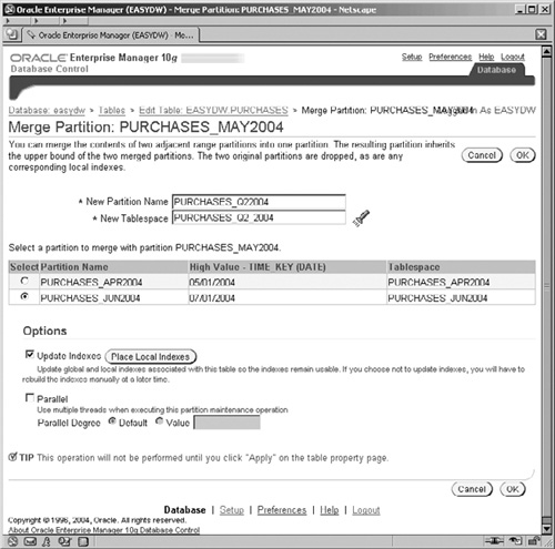
The operation is then repeated to merge the new partition for Q22004 with the partition for APR2004.
When merging partitions, both the data and the indexes are merged. The index partitions for April, May, and June were automatically dropped and were replaced by a new index partition for Q2. In the following query, there is a new index partition, PURCHASES_Q22004, for the indexes on the PURCHASES table.
SELECT index_name, partition_name, status
FROM   user_ind_partitions;

INDEX_NAME               PARTITION_NAME    STATUS
------------------------ ----------------- --------
PURCHASE_SPECIAL_INDEX   PURCHASES_Q22004  UNUSABLE
PURCHASE_CUSTOMER_INDEX  PURCHASES_Q22004  UNUSABLE
PURCHASE_PRODUCT_INDEX   PURCHASES_Q22004  UNUSABLE
PURCHASE_TIME_INDEX      PURCHASES_Q22004  UNUSABLE
The new index partitions are unusable and must be rebuilt, as shown in the following example.
ALTER INDEX purchase_product_index
  REBUILD PARTITION purchases_q22004 ;
ALTER INDEX purchase_time_index
  REBUILD PARTITION purchases_q22004 ;
ALTER INDEX purchase_special_index
  REBUILD PARTITION purchases_q22004 ;
ALTER INDEX purchase_customer_index
  REBUILD PARTITION purchases_q22004 ;
If a partition becomes too big, it may need to be split to help maintenance operations complete in a shorter period of time or to spread the I/O across more devices. A partition can be split into two new partitions. If the PURCHASES table was originally partitioned by quarter, and sales significantly exceeded expectations resulting in a very large partition, the partition could be split up into three monthly partitions. Tablespaces are first created for PURCHASES_APR2004, PURCHASES_MAY2004, and PURCHASES_JUN2004.
In the following example, all rows with PURCHASE_DATE less than or equal to May 1, 2004, will be split into the PURCHASES_APR2004 partition. The remaining rows will remain in the PURCHASES_Q22004 partition. The April purchases will be stored in the PURCHASES_ APR2004 tablespace.
ALTER TABLE purchases
SPLIT PARTITION purchases_q22004
     AT (TO_DATE('01-MAY-2004','dd-mon-yyyy'))
     INTO (PARTITION purchases_apr2004
             TABLESPACE purchases_apr2004,
           PARTITION purchases_q22004) ;
After the split operation, there are two partitions. Next, the remaining rows in the partition, PURCHASE_Q22004, are split into the May and June partitions.
ALTER TABLE purchases
SPLIT PARTITION purchases_q22004
     AT (TO_DATE('01-JUN-2004','dd-mon-yyyy'))
     INTO (PARTITION purchases_may2004
              TABLESPACE purchases_may2004,
           PARTITION purchases_jun2004
              TABLESPACE purchases_jun2004) ;
The data has been repartitioned, and the PURCHASES_Q22004,z partition automatically dropped, as shown in Figure 11.34.

This operation is performed from EM via the Edit Table, Partition screen, for the PURCHASES table, as shown in Figure 11.35, by selecting the Split action. The use of the screen to perform this operation is much more intuitive and less error prone than performing the operation by hand with SQL commands.

Clicking the OK button returns you to the Partitions screen, with check boxes against the partition to indicate that the actual split operation is pending. Repeat the operation again on the PURCHASES_Q22004 partitions to split it for the May and June partitions. When the Apply button is clicked, the two pending split partition operations are actually performed.
Any partitions of the local indexes corresponding to the PURCHASES_ Q22004 partition have been dropped. In their place are new local index partitions for the new table partitions.
SELECT INDEX_NAME, PARTITION_NAME, STATUS
FROM   USER_IND_PARTITIONS;

INDEX_NAME              PARTITION_NAME     STATUS
----------------------- ------------------ --------
PURCHASE_SPECIAL_INDEX  PURCHASES_APR2004  UNUSABLE
PURCHASE_CUSTOMER_INDEX PURCHASES_APR2004  UNUSABLE
PURCHASE_SPECIAL_INDEX  PURCHASES_JUN2004  UNUSABLE
PURCHASE_SPECIAL_INDEX  PURCHASES_MAY2004  UNUSABLE
PURCHASE_CUSTOMER_INDEX PURCHASES_JUN2004  UNUSABLE
PURCHASE_PRODUCT_INDEX  PURCHASES_APR2004  UNUSABLE
PURCHASE_TIME_INDEX     PURCHASES_APR2004  UNUSABLE
PURCHASE_CUSTOMER_INDEX PURCHASES_MAY2004  UNUSABLE
PURCHASE_PRODUCT_INDEX  PURCHASES_JUN2004  UNUSABLE
PURCHASE_PRODUCT_INDEX  PURCHASES_MAY2004  UNUSABLE
PURCHASE_TIME_INDEX     PURCHASES_JUN2004  UNUSABLE
PURCHASE_TIME_INDEX     PURCHASES_MAY2004  UNUSABLE
Any unusable indexes must be rebuilt, as follows, for the APR2004 partition.
ALTER INDEX purchase_product_index
    REBUILD PARTITION purchases_apr2004 ;
ALTER INDEX purchase_time_index
    REBUILD PARTITION purchases_apr2004 ;
ALTER INDEX purchase_customer_index
    REBUILD PARTITION purchases_apr2004 ;
ALTER INDEX purchase_special_index
REBUILD PARTITION purchases_apr2004 ;Range and list partitions can be merged, but hash partitions cannot; they must be coalesced. Rather than determining which partition a row is stored in by comparing the value of the partitioning key with the table’s partitioning criteria, as is done for range or list partitioning, the partition is determined by applying a hash function.
Merging partitions in effect reduces the number of partitions by one. When the number of partitions changes, the hash function must be reapplied to redistribute the data. Coalescing the partitions does this.
The following example shows the creation of a hash-partitioned table with 10 partitions.
CREATE TABLE easydw.hash_purchases
 (product_id                   varchar2(8),
  time_key                     date,
  customer_id                  varchar2(10),
  purchase_date                date,
  purchase_time                number(4,0),
  purchase_price               number(6,2),
  shipping_charge              number(5,2),
  today_special_offer          varchar2(1))
PARTITION BY HASH(product_id)
PARTITIONS 10;
To reduce the number of partitions by one, issue the following command.
ALTER TABLE easydw.hash_purchases COALESCE PARTITION;
This, in effect, drops a partition.
Likewise, a hash-partitioned table cannot be split when it becomes too big. To increase the number of partitions in a hash-partitioned table, alter the table and add a partition to it.
Sometimes we need to remove all the rows in a partition. For example, we may only keep 18 months of data and, once a month, we need to remove that old data. Rather than delete each row individually, we can use the TRUNCATE PARTITION option, which rapidly removes the data.
To remove all the rows from a partition, but not the partition itself, use TRUNCATE partition. This is much faster than deleting each row in the partition individually. Any local indexes for the partition, such as the EASYDW.PURCHASE_TIME_INDEX, are also truncated. Prior to truncating the partition, there are 3,847 rows in the PURCHASES_JAN2003 partition.
SELECT COUNT(*) FROM purchases
WHERE time_key
        BETWEEN TO_DATE('01-JAN-2003', 'dd-mon-yyyy')
            AND TO_DATE('31-JAN-2003', 'dd-mon-yyyy') ;

  COUNT(*)
----------
      3847

ALTER TABLE PURCHASES TRUNCATE PARTITION purchases_jan2003;
After truncating the partition, all rows have been deleted.
SELECT COUNT(*) FROM purchases
WHERE time_key
        BETWEEN TO_DATE('01-JAN-2003', 'dd-mon-yyyy')
            AND TO_DATE('31-JAN-2003', 'dd-mon-yyyy') ;

  COUNT(*)
----------
         0
The EM screen for this operation is shown in Figure 11.36; it is a confirmation screen, which provides some useful options and control over the truncate operation. When a truncate command is performed, it deletes the rows, but you can specify whether the freed-up space is retained by the partition or returned to the containing tablespace.
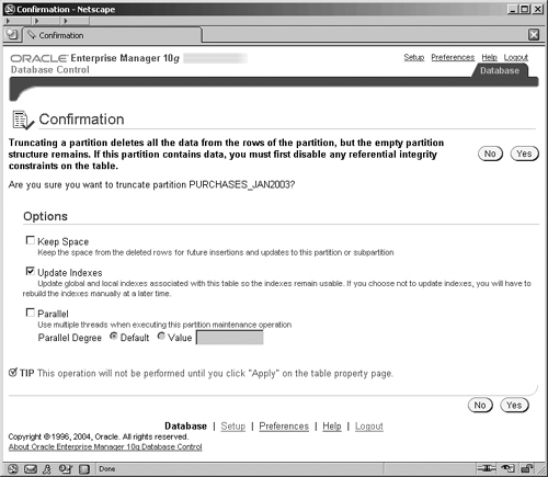
Be warned that the truncation operation is actually a DDL operation, which effectively commits immediately and does not create any undo information. So once you click the Yes button, you confirm the operation and lose your data.
A partition can be moved from one tablespace to another. For example, if the January partition on the PURCHASES table had been incorrectly created in EASYDW_DEFAULT tablespace, it would need to be moved to the PURCHASES_JAN2003 tablespace to be consistent with the database design conventions. The following command could be used.
ALTER TABLE purchases
     MOVE PARTITION purchases_jan2003
     TABLESPACE purchases_jan2003 ;
Hint
A NOLOGGING clause can be specified after the tablespace name; that causes the operation not to create redo logs and results in better performance. After performing NOLOGGING operations, don’t forget to take a backup, since you will not be able to recover in the event of media failure.
This task can also be performed in EM, where you are asked simply to specify the target tablespace. It also provides the option to update the indexes and choose the degree of parallelism to be used for the move operation.
Most of the management operations that can be performed at a table level can also be performed on an individual partition or subpartition of a table. Partitions or subpartitions can be backed up, exported, restored, and recovered without affecting the availability of the other partitions or subpartitions. To best manage each partition or subpartition independently, they should each be stored in their own tablespace. Each tablespace should be stored on one or more separate storage devices.
Summary management and the query optimizer make use of the fact that the data is partitioned in choosing the optimal strategy for executing a query or refreshing a materialized view. Partition Change Tracking (PCT) for materialized views, which was discussed in Chapter 7, keeps track of which partitions have been updated after a partition maintenance operation and recomputes only that portion of the materialized view when it is refreshed. Partition Change Tracking also increases the query rewrite capabilities of the materialized view by rewriting queries to use the partitions of the materialized view that are not stale. If a table is partitioned, the query optimizer can use partition elimination or partition pruning to determine if a certain query can be answered by reading only specific partitions.
Hint
The examples shown in this section have performed partition maintenance operations on a table, but don’t forget that partitions are also used on indexes, so you will have to create and maintain the corresponding index partitions. Also in these examples we’ve used partitions, but the operations are equally valid on subpartitions as well.
Probably one of the aspects of the design that will be changed is the indexes. New ones will be created, and existing ones will be modified. In a data warehouse, there is a temptation to create more indexes, because of the lack of updates to the system. However, you should consider the impact all of these indexes will have on the data load time.
If you need to rebuild an index for any reason, it is suggested that you use the ALTER INDEX REBUILD statement, which should offer better performance than dropping and recreating the index.
Many table maintenance operations on partitioned tables invalidate global indexes and they are marked UNUSABLE. You must then rebuild the entire global index or, if partitioned, all of its partitions. To avoid this you can include the UPDATE GLOBAL INDEXES clause in the ALTER TABLE statement for the maintenance operation. Specifying this clause tells Oracle to update the global index at the time it executes the maintenance operation DDL statement.
With the increased importance of our data warehouse to the business can come the increased requirement for it to be constantly available; when it is not actually open to the users, it will need to be refreshed. These activities can seriously reduce the available window in which to perform maintenance operations. In a data warehouse with very large tables, these operations can be quite time consuming to perform. Gone are the days when the warehouse was only needed 9 to 5 and then there were these long batch windows and periods when maintenance could be performed. Now data warehouses are being used 24 hours a day, and it is becoming increasingly difficult to find time to perform maintenance operations.
However, Oracle has online redefinition, which enables tables to be rebuilt and restructured and data to be transformed while the tables are fully on-line and accessible to the users of the database.
The benefits and features of online redefinition are:
The ability to change the table to or from a partitioned structure
To improve space utilization
To modify the storage characteristics of the table
To change a normal table to or from an index-organized table
To Automatically copy dependant objects on the table, such as triggers, constraints, and indexes (new in 10g)
Dependant stored procedures do not require recompilation (new in 10g)
To free unused space within the table segments back to the tablespace (new in 10g)
To convert data types such as longs to LOBs (new in 10g)
In spite of all the care and attention spent during the design and deployment of our warehouse, there can still be the occasional table that is created but does not operate quite as anticipated. This could be due to a number of reasons, such as:
The table has become much larger than expected by the volume metrics on which the warehouse designer based physical table design, and it now needs to be partitioned.
The update activity on the table was not as expected during analysis and has caused the underlying physical storage to be used inappropriately.
In our first example, changing a large table to be partitioned enables easier management and performance improvements to the queries that access it—for example, to make use of partition elimination or partition-wise joins. A persistent problem that exists with table partition operations is that it is not possible to convert an unpartitioned table into a partitioned table. There is no SQL operation to do this. All of the partition operations that we discussed earlier in the chapter are only possible if the table was originally implemented as a partitioned table.
In the second example for storage problems, unanticipated update DML activity can cause a problem called row chaining, which causes a row to become stored in more than one disk block and consequently require two I/O operations to retrieve it.
Correcting these types of problems typically requires that the table be dropped, rebuilt, and reloaded to restructure it or improve the space utilization. But if the table has constraints or triggers on it, then the opportunity to drop the table in order to rebuild it in this fashion is significantly reduced.
Online redefinition enables these changes to the table structure and storage to be performed without needing to drop the table. During the operation the table remains available and in use by the users.
There are two ways to use on-line redefinition: from within Enterprise Manager or by invoking the DBMS_REDEFINITION package directly. We will start by looking at the Enterprise Manager approach, but because this currently only offers a limited subset of what is possible via the package, we will then look at an example that calls the package directly.
Within Enterprise Manager, the on-line redefinition wizards can be accessed by going to the Maintenance screen and clicking on the Reorganize Objects link. On the first screen of the wizard (not shown), you need to decide which path through the wizard you want to take to reorganize the objects:
By schema
By tablespace
Either route enables you to specify the objects within the schema or tablespace that you want to reorganize.
The wizard is very easy to use and very self-explanatory. One of the important screens is the Options screen, shown in Figure 11.37, which requires further explanation.
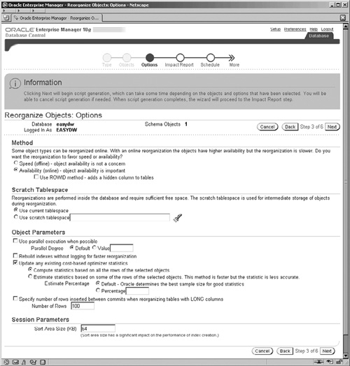
There are two methods by which the objects can be rebuilt:
Offline, which results in the objects being unavailable
Online, which ensures that the objects are available during the redefinition process
The online method requires the tables to have some form of unique identifier, such as a primary key, rowid, or unique index. If one is not present, then you will need to tick the check box for the ROWID method.
As part of the redefinition process, temporary objects will need to be built; therefore, the tablespace reorganization method needs to use a separate scratch tablespace.
There are two final sections on the Options screen shown in Figure 11.37: Object Parameters and Session Parameters, which enable you to fine-tune the execution of the redefinition. In these sections, you can control the degree of parallelism to be used, which can be important for large objects. Similarly, when indexes are being rebuilt, if the check box to build without generating redo logs is selected, a performance gain can be achieved for large indexes. However, be careful when selecting NOLOGGING, because this can prevent database recovery in the event of media failure; taking a backup is advised.
When the Next button, shown in Figure 11.37, is clicked, the wizard analyzes the objects and dependencies that you have selected and displays an impact report (not shown) of its findings. Examples of the types of findings detected are insufficient tablespace or no primary key on a table for an on-line redefinition method. After viewing the report, you then have the option to go back and make corrections using the Back button or progress to the Schedule screen by pressing the Next button.
The final two steps of the wizard are to specify the schedule for when you want the reorganization performed (this screen is not shown) and to make a final review of the process that you have defined via the wizard. On the Review page, which is shown in Figure 11.38, the scripts that are generated by Enterprise Manager are displayed.
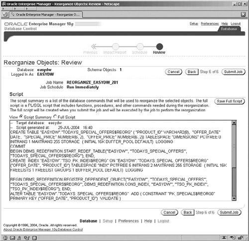
The scripts produced in Figure 11.38 are either:
A summary showing the steps required and the packaged procedures called
The full script, which is detailed PL/SQL and includes much more code for controlling each step of the operation
It is the full script that is actually executed. The summary script, however, is very useful as a starting point for understanding more about the steps required for the redefinition operation.
Clicking on the Submit Job button, shown in Figure 11.38, will submit the job to the job queue for execution according to the schedule that you defined.
From the initial part of the script shown in Figure 11.38, it is clear that a number of steps are required for redefining an object; these are performed by executing various procedures in the DBMS_REDEFINITION package.
Before attempting to redefine a table, you should use the procedure DBMS_REDEFINITION.CAN_REDEF_TABLE() to check if a redefinition is possible. This is because, at the time of writing, there is a limitation with the DBMS_REDEFINITION package in that it is not possible to reorganize a table that has materialized views on it.
We will illustrate the use of this feature with an example. Suppose the CUSTOMER table is currently not partitioned. However, as the business grows, this table has grown significantly in size and so we would now like to reorganize it to use list partitioning on the STATE column. Further, we would like to change the OCCUPATION column from a VARCHAR2(15) to a VARCHAR2(20). Finally, in order to support some more detailed analysis of the postal code for U.K. addresses, we want to restructure it from a single column into two columns. We will split it on the first space it may contain into OUTER and INNER parts, as follows:
If the postal code contains a space, then the OUTER part will be assigned the characters preceding the first space and the INNER part will be assigned the characters following the first space.
For example, W1 1QC becomes OUTER=W1 and INNER=1QC
If the postal code contains no space, then it is assigned to the OUTER column and the INNER column is null.
For example, 73301 becomes OUTER=73301 and INNER=NULL
To perform the split of the postal code we need to define two PL/SQL functions to perform the operations, as follows:
CREATE OR REPLACE
FUNCTION outer(postal_code IN VARCHAR2)
RETURN VARCHAR2
IS
BEGIN
  IF instr(postal_code, ' ') = 0
  THEN return (postal_code);
  ELSE return (substr(postal_code,
                      1,
                      instr(postal_code, ' ')-1)) ;
  END IF ;
END ;

CREATE OR REPLACE
FUNCTION inner(postal_code IN VARCHAR2)
RETURN VARCHAR2
IS
BEGIN
  IF instr(postal_code, ' ') = 0
  THEN return (null);
  ELSE return (substr(postal_code,
                      instr(postal_code, ' ')+1)) ;
  END IF ;
END ;
To redefine the CUSTOMER table, while allowing users to still query and update the data, we need to do the following.
Create the interim table showing how you would like the redefined table to look. Note that the interim table will need to have a name different from the actual table you are redefining.
CREATE TABLE customer_interim
(
 CUSTOMER_ID          VARCHAR2(10) NOT NULL,
 CITY                 VARCHAR2(15),
 STATE                VARCHAR2(10),
 POSTAL_CODE_OUTER    VARCHAR2(10),
 POSTAL_CODE_INNER    VARCHAR2(10),
 GENDER               VARCHAR2(1),
 REGION               VARCHAR2(15),
 COUNTRY              VARCHAR2(20),
 TAX_RATE             NUMBER,
 OCCUPATION           VARCHAR2(20)
)
PARTITION BY LIST(state)
(
  PARTITION northeast VALUES ('NH', 'VT', 'MA', 'RI', 'CT'),
  PARTITION southeast VALUES ('NC', 'GA', 'FL'),
  PARTITION northwest VALUES ('WA', 'OR'),
  PARTITION midwest VALUES   ('IL', 'WI', 'OH'),
  PARTITION west VALUES      ('CA', 'NV', 'AZ'),
  PARTITION otherstates VALUES (DEFAULT)
);Call the START_REDEF_TABLE procedure providing the name of the table to be redefined and the interim table.
BEGIN
 dbms_redefinition.start_redef_table
   (uname=>'EASYDW',
    orig_table=>'CUSTOMER',
    int_table=>'CUSTOMER_INTERIM',
    col_mapping=>'customer_id customer_id, '
               ||'city city, '
               ||'state state,'
               ||'outer(postal_code) postal_code_outer,'
               ||'inner(postal_code) postal_code_inner,'
               ||'gender gender, '
               ||'region region, '
               ||'country country, '
               ||'tax_rate tax_rate, '
               ||'occupation occupation'
   );
END;
Once you have done this, the interim table will be instantiated with the contents of the original table.
Currently, the Enterprise Manager wizard does not support the more complex table redefinitions that we are performing—for example, where new columns are added, dropped or column values are transformed. These types of operations require a mapping and transformation between the columns on the original table and the columns on the interim table and are performed by using the COL_MAPPING parameter.
The COL_MAPPING parameter takes a list of comma-separated pairs of columns. The first column in each pair is the original table column, or a function on the original table column. The second column in a pair is the destination column in the interim table to which we are mapping. In our example, outer(POSTAL_CODE) from the original table is mapping to POSTAL_CODE_OUTER in the interim table.
If the column mapping parameter isn’t supplied, then it is assumed that all columns map with their names unchanged to columns in the interim table.
For each dependent object, such as grants, triggers, constraints, and indexes:
If the object is the same on the interim table as it is on the table being redefined, then call the COPY_TABLE_DEPENDENTS procedure to automatically create it on the interim table.
If it is different on the interim table, then manually create it and call the REGISTER_DEPENDENT_OBJECT procedure. This registers and associates the two names of the object as applied on the two tables. This enables the objects to be correctly renamed upon completion of the redefinition.
In our example, all dependent objects are the same on the interim table, so we are using the COPY_TABLE_DEPENDENTS procedure, as follows:
set serveroutput on

DECLARE
   num_errors number;
BEGIN
   num_errors:= 0;
   dbms_redefinition.copy_table_dependents
      (uname=>'EASYDW',
       orig_table=>'CUSTOMER',
       int_table=>'CUSTOMER_INTERIM',
       num_errors=>num_errors);
   dbms_output.put_line
      ('Number of errors:'||to_char(num_errors));
END;Call the SYNC_INTERIM_TABLE procedure, which will synchronize any DML performed on the original table with the interim table. Any changes done to the original table, while it is being redefined, will be automatically tracked by Oracle and applied to the interim table.
BEGIN
  dbms_redefinition.sync_interim_table
     (uname=>'EASYDW',
      orig_table=>'CUSTOMER',
      int_table=>'CUSTOMER_INTERIM'),
END;Call the FINISH_REDEF_TABLE procedure to finish the redefinition. Finishing the redefinition ensures that all of the indexes, grants, and triggers are on the redefined table, and the referential integrity constraints and triggers are enabled.
BEGIN
  dbms_redefinition.finish_redef_table
     (uname=>'EASYDW',
      orig_table=>'CUSTOMER',
      int_table=>'CUSTOMER_INTERIM'),
END;BEGIN
dbms_stats.gather_table_stats(ownname=>'easydw',
tabname=>'customer',
cascade=true
);
END;Hint
If the on-line redefinition operation fails for any reason, then the ABORT_REDEF_TABLE procedure must be called; this cleans up all the dependent objects so you can start again.
Our table structure has now changed, and, if we look at a subset of the new postal code columns, we can see that they have been correctly transformed and contain their new values.
SQL> desc customer
 Name                    Null?    Type
 ----------------------- -------- ----------------
 CUSTOMER_ID             NOT NULL VARCHAR2(10)
 CITY                             VARCHAR2(15)
 STATE                            VARCHAR2(10)
 POSTAL_CODE_OUTER                VARCHAR2(10)
 POSTAL_CODE_INNER                VARCHAR2(10)
 GENDER                           VARCHAR2(1)
 REGION                           VARCHAR2(15)
 COUNTRY                          VARCHAR2(20)
 TAX_RATE                         NUMBER
 OCCUPATION                       VARCHAR2(20)

SQL> SELECT postal_code_outer outer, postal_code_inner inner
     FROM customer;

OUTER      INNER
---------- ----------
10001
W1         1QC
W1         1QC
W1         1QC
10001
W1         1QC
73301
W1         1QC
We think you will agree that the on-line redefinition feature is a very useful and powerful tool to assist the administrator with the long-term management of the warehouse tables.
As the tables in our warehouse undergo INSERT, UPDATE and DELETE operations, the underlying space in the tablespace segments can become less efficient and space can become unusable. A new feature in Oracle Database 10g, called on-line segment shrink, enables this space to be reclaimed from a table and reassigned back to the tablespace for reuse.
In previous versions of the database, this operation would have involved a costly rebuild of the table, which would mean that it became unavailable. However, in Oracle Database 10g the operation can be performed while the table and indexes are on-line and fully available for use.
Via SQL, segment shrinkage can be performed by simply altering the table, index, or materialized view by using the SHRINK SPACE command. For example:
ALTER MATERIALIZED VIEW product_sum SHRINK SPACE;
Hint
To perform the shrink space operation, the owning tablespace must be set for automatic segment management, and tables and materialized views must be altered to enable row movement.
In Enterprise Manager, one of the new advisors is the Segment Advisor, which can be accessed from Advisor Central. This advisor will analyze objects you specify, either those owned by a schema or those residing in the same tablespace, and provide a report of the space usage and what can be reclaimed. It then enables you to schedule the job on the objects that you have selected for shrinkage.
Rather than a hit and miss manual approach for finding out where space can be effectively recovered, the Segment Advisor provides a very quick and easy method to access and perform this operation.
An extremely important management task is refreshing the warehouse with the latest data. This is a management task that is usually performed overnight with the data presented in batches. As was described earlier, frequently the data has to be cleansed and transformed before it can be loaded. Chapter 5 described various techniques that can be used for loading the new data into the warehouse.
Throughout this book, we have seen extensive use of Oracle Enterprise Manager for managing and controlling many of our management tasks. Depending on how complex your tasks are and on the data dependencies, you may prefer to use your own techniques. Otherwise, you could place the jobs on the Scheduler queue and come in the next day to see that everything has run smoothly. For example, it is not uncommon to receive data loads from various sources at different times. If there are dependencies between the data, then you may have to control that within your own management suites. Alternatively, Oracle Warehouse Builder performs complex scheduling of its various tasks by use of Oracle Workflow.
Once the data has been loaded into the warehouse, the materialized views must be refreshed. Depending on the number of materialized views, this could also take a significant amount of time.
An OEM job could be created to refresh the materialized views. Executing the DBMS_MVIEW.REFRESH_ALL_MVIEWS procedure could refresh all of the materialized views. Alternatively, you could use the DBMS_MVIEW.REFRESH_DEPENDENT option to request that it refresh only materialized views dependent on certain tables. Or you can call the refresh procedure and specify which materialized views are to be refreshed. Specific details on how to refresh materialized views were described in Chapter 7.
Missing or stale optimizer statistics are often the cause of suboptimal query performance. The cost-based optimizer uses statistics such as the cardinality of the table, number of distinct values of a column, and the data distribution to determine the cost of an access path. The cost is a measure of how much I/O, CPU time, and memory will be required to execute the query. To use the cost-based optimizer effectively, statistics describing the cardinality and data distribution must be collected for each table, index, and materialized view.
Previously, to automate the gathering of statistics for a table meant enabling the monitoring of DML activity for that table using the MONITORING keyword in the CREATE or ALTER TABLE command. Then the GATHER STALE option in the GATHER_DATABASE_STATS procedure was used to gather statistics for just those tables whose contents had changed significantly.
Starting with Oracle Database 10g, the MONITORING and NOMONITORING keywords have been deprecated, and now statistics collection is performed automatically and is controlled by the STATISTICS_LEVEL initialization parameter. When this parameter is set to BASIC, the monitoring and automatic statistics collection is disabled, and when set to TYPICAL (the default), it is enabled. Monitoring tracks the insert, update, and delete activity on the tables and maintains the information in the SGA; it then periodically updates this information into the data dictionary.
Finally, there is an automatic statistics collection job that is available “out of the box” with the Scheduler. Only the user SYS can see and configure this job. Log on to Enterprise Manager as SYS and navigate to the Administration page, and click the Jobs link in the Scheduler section; this will display the Scheduler Jobs page where the GATHER_STATS_JOB will be listed. This job is scheduled using one of two windows:
WEEKNIGHT_WINDOW for weekdays from 10:00 P.M. to 6:00 A.M.
WEEKEND_WINDOW from midnight Saturday morning for 48 hours
You can, of course, still manually perform statistics collection. Two methods are available:
Via Enterprise Manager using the Gather Statistics wizard
Via the DBMS_STATS package
To access the wizard go to the Maintenance Home screen and, in the Utilities section, click on the Gather Statistics link. This displays a five-step wizard, which enables a job to be defined and scheduled to collect statistics on:
Schemas
Tables
Indexes
Table partitions
Index partition
The whole database
Alternatively, you can use the DBMS_STATS package directly. For example, to use the DBMS_STATS package to collect statistics on all tables and indexes in the EASYDW schema, issue the following query:
EXECUTE DBMS_STATS.GATHER_SCHEMA_STATS ('EASYDW'),If you are just interested in a specific table—PURCHASES, for example—you can use the following statement. This will gather statistics on the table, its columns, and indexes.
EXECUTE DBMS_STATS.GATHER_TABLE_STATS ('EASYDW', 'PURCHASES'),The table and column statistics can be viewed by querying the USER_TABLES and USER_TAB_COLS dictionary views, as follows:
-- table statistics
SELECT num_rows, blocks, avg_row_len, last_analyzed
FROM   user_tables
WHERE  table_name = 'PURCHASES';

  NUM_ROWS     BLOCKS AVG_ROW_LEN LAST_ANAL
---------- ---------- ----------- ---------
     94619        567          42 13-JUL-04
-- column statistics
SELECT column_name, num_distinct, num_nulls, avg_col_len
FROM   user_tab_cols
WHERE  table_name = 'PURCHASES';

COLUMN_NAME         NUM_DISTINCT NUM_NULLS AVG_COL_LEN
------------------- ------------ --------- -----------
PRODUCT_ID                   165         0           7
TIME_KEY                     762         0           8
CUSTOMER_ID                  500         0           9
SHIP_DATE                    762         0           8
PURCHASE_PRICE                 9         0           5
SHIPPING_CHARGE                3         0           4
TODAY_SPECIAL_OFFER            2         0           2
To collect statistics for the index, CUSTOMER_INDEX, use the following statement:
EXECUTE DBMS_STATS.GATHER_INDEX_STATS
            ('easydw', 'purchase_customer_index'),
Statistics should be gathered after data is loaded and again whenever changes made to the data are likely to have altered the distribution. This ensures that the cost-based optimizer has up-to-date data to base its decision upon. When partitioned tables are used, only the newest partition or subpartition to which rows have been added needs to be analyzed for statistics. For example, if a new partition for Jan 2005 was added to the purchases table, statistics can be collected for the newly added partition, as follows:
ALTER TABLE purchases
  ADD PARTITION purchases_jan2005
  VALUES LESS THAN (TO_DATE('01-02-2005',
                            'DD-MM-YYYY'));

INSERT /*+APPEND */  INTO purchases ...

EXECUTE DBMS_STATS.GATHER_TABLE_STATS
('easydw', 'purchases', 'purchases_jan2005'),System statistics such as CPU speed and number of I/Os per second give an indication of the resource availability in the system. Oracle Database 10g considers system statistics in determining the execution plan. This allows the optimizer to make smarter decisions when several users are contending for the same resources. System statistics can be collected using the DBMS_STATS.GET_SYSTEM_STATS procedure.
As with all statistics, it is important that the system statistics give the optimizer an accurate picture of the system load. Statistics could be collected for different periods during the day—for example, during normal business hours and during after-hours reporting activities. Statistics can be saved using the EXPORT_SYSTEM_STATS procedure and later imported into a database using the IMPORT_SYSTEM_STATS procedure.
In the Oracle Database 10g, a feature known as dynamic sampling can be used by the optimizer when statistics on a table are absent. With dynamic sampling, the optimizer automatically collects statistics by sampling the data before optimizing the query. Dynamic sampling is useful for queries whose tables do not have statistics collected or when the statistics are too old.
To enable dynamic sampling, the initialization parameter, OPTIMIZER_DYNAMIC_SAMPLING, must be set to a value greater than 1. The optimizer will perform dynamic sampling if there is more than one table in the query and some of the tables have no statistics and no indexes. Note that dynamic sampling will incur some overhead during query optimization and hence must be used with care. In a data warehouse, it is always a good practice to collect statistics on all your tables as part of your housekeeping procedures and to keep them current.
Throughout this book, the typically large size of the data warehouse means that tasks can take a very long time to complete. So far, we have considered some techniques for improving performance, but there is a very useful one that is worth mentioning again: the ability to run operations in parallel.
Parallel execution is most useful for operations that access significant amounts of data, including queries, index creation, bulk inserts, updates and deletes, aggregations, and data movement. At the time of writing, most operations can be run in parallel, including:
Parallel query—queries and subqueries in SELECT statements.
Parallel DDL—including:
CREATE TABLE AS SELECT, CREATE INDEX, and ALTER INDEX REBUILD
For partitioned tables: ALTER TABLE MOVE, SPLIT, COALESCE
For partitioned indexes: ALTER INDEX REBUILD or SPLIT
Parallel DML—INSERT, UPDATE, DELETE, multitable insert
SQL*Loader and external tables
Parallel operations require accurate statistics to perform optimally and correct use of the initialization parameters to ensure that parallel operations properly utilize the database resources. Chapter 6 discussed in detail the configuration of the database to use parallelism and its use to improve query performance, and Chapter 5 showed examples of loading data in parallel. Similar techniques are used to execute DDL statements in parallel.
One should not forget the security of the data in a data warehouse. In many respects, warehouse data should probably be more secure than production data, because its value to your competitors could be enormous. Imagine if one of your users started earning spare cash by running reports against your data or if an employee left the company with information from the data warehouse. If you are laughing at the last statement, please don’t; although it is very rare, it actually does happen.
The level of security in your data warehouse will depend on what you think is appropriate for your system. Some sites may prefer to have the warehouse open for read-only queries, but restrict management tasks such as creating summary data to the administration team.
We have already seen, in Chapter 2, how we can protect individual tables by specifying explicitly who may access the tables using the GRANT and REVOKE commands.
Another technique is to create a role, assign privileges to that role, and then grant that role to a user. Roles can either be created via SQL or by going to the Administration screen and following the Roles link in the Security section, which will take you to the Roles screen. Here you will see a list of all of the existing roles in the database and from where you can perform a number of actions to create and administer roles and view to which users the role has been granted.
Click the Create button and you will navigate to the General tab of the Create Role screen, shown in Figure 11.39, where the name of our new role, EASY_USER, is entered.

Security isn’t limited only to tables; it can be placed on a wide range of database objects. Clicking on the links on this page displays specific screens that enable objects of that type to be granted to our new role. For example, to grant privileges on EASYDW tables to this role, click on the Object Privileges link and you will see a screen similar to that shown in Figure 11.40. We have already granted the SELECT privilege on the PRODUCT and CUSTOMER tables to the role by choosing the object type, which in this example is a table, and clicking the Add button. The subsequent simple screen (not shown) enables you to find the objects and assign the privileges.

Figure 11.40 also shows the range of objects for which privileges can be granted. The screens for granting the other privilege types to the role operate in a similar fashion.
For those of you who do not want to use Enterprise Manager to create the role—for example, if you want to perform this at a later time—the Show SQL button will display a screen that shows the commands to implement this role.
Once the role has been defined, it can be allocated to a user, as shown in Figure 11.41. From the Administration screen go to the Security section, follow the Users link, and navigate to the Edit Users screen. Select the user account and click on the Roles link. By clicking on the Modify button you can assign the new EASY_USER role in the subsequent screen. The Admin Option shown here designates whether or not the user that you are assigning the role to can grant that to another user. For our warehouse security, checking the Admin Option box would allow access to the warehouse to be granted to users outside of the administrator’s control and is not a good idea.
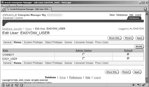
Roles are an extremely powerful feature in Oracle and can save an immense amount of time in not having to allocate lots of individual privileges to a user.
Applications that are deployed on the Internet and make information available to customers, suppliers, employees, or other users need to provide access control at a very fine level of granularity. An on-line banking system needs to ensure that customers can only see transactions for their accounts, and not anyone else’s account. A self-service human resources application may let employees see their own records and modify their marital status, address, and phone number, but not their salary. The same application may provide managers with the ability to read and modify the records of all employees who work for them.
As companies are increasing focus on their core competencies, they may outsource other tasks, such as human resources, customer support, and payroll. When designing an application that provides hosting services, the data for each company must be kept separate and secure from each other.
Traditionally, access has been controlled at the object level. The data security policy determines which users have access to which schema objects, and which types of actions are allowed for each object. For example, a user may be able to select from a table, but not insert, update, or delete the rows in the table. If you wanted to allow a user access to a subset of rows in a table, a view could be created and the user granted access to the view. If you have a self-service application, where each employee in a large company had access to the rows containing his or her own personal data in the human resources database, each employee would have to have his or her own view. However, the number of views quickly becomes unwieldy. If you want to allow access to employee data for a certain group of users only through the human resources application, and not for adhoc queries, views do not give you this capability.
Another way to implement data security is with Virtual Private Database (VPD) and finegrained access control. VPD provides row level security, for all applications. Associating one or more security policies with a table or view creates the Virtual Private Database. Any access to a table with an attached security policy causes the invocation of a function that implements the policy. The function returns an access condition in the form of a WHERE clause, which is appended to the user’s SQL statement, thus dynamically modifying the user’s data access. For example, in the EASYDW warehouse, we could allow each customer to see information about his own order history on-line. When a customer issues SELECT * FROM PURCHASES, the function would add his or her customer_id to the WHERE clause, resulting in the following query.
SELECT * FROM PURCHASES WHERE customer_id = 'AB123459'
Often, you want to control access based on some attributes about the user, such as job code, department, location, or whether he or she is a customer or partner. An application context is created to do this. Upon logging into the database, the application context is associated with the user’s session. Each application can have its own application context, with each having different attributes.
After creating the application context, the PL/SQL functions to implement the security policies are created. The function determines the WHERE clause to return, based on the user’s application context.
The PL/SQL package DBMS_RLS, is used to administer the security policies and apply them to the appropriate tables. Using this package, you can add, drop, enable, disable, and refresh the policies you create.
Many of the Oracle applications make use of VPD to provide finegrained access control.
A very important piece of information for the DBA is to know how much space is available in the data warehouse. One technique to avoid running out of space is to create the datafiles with autoextend and to define an unlimited number of extents. However, this won’t help you if the disk actually fills up.
Therefore, as part of your routine monitoring of the data warehouse, you should check for free space. This could be done by simply navigating to the Tablespaces screen, where this information is shown by default, or you may prefer to simply query the Oracle metadata in the data dictionary for this information. Figure 11.42 shows an example of the space utilization for the EASYDW database.
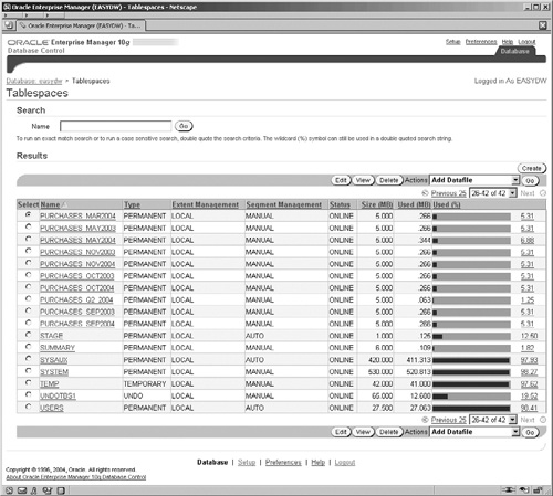
In Figure 11.42, the Used (%) graph display for each tablespace enables a very quick visual check of how much space has been used in the tablespace. In our example, we can see that SYSAUX, SYSTEM, TEMP, and USERS are very nearly full; this may cause a problem for any operations that cause an object in these tablespaces to grow in size. However, this screen does not quite show the full story, because, you will recall from Chapter 2 (see Figure 2.21), the datafiles for a tablespace can be set to auto extend when they are nearly full. We will need to click on the tablespace name link and drill down to the data file to verify the exact status.
But manually checking this on a daily basis is a chore and prone to error; with Oracle Database 10g, this type of operation is now performed automatically. To look at this further, click on the All Metrics link in the Related Links of the Home pages to display the screen shown in Figure 11.43.
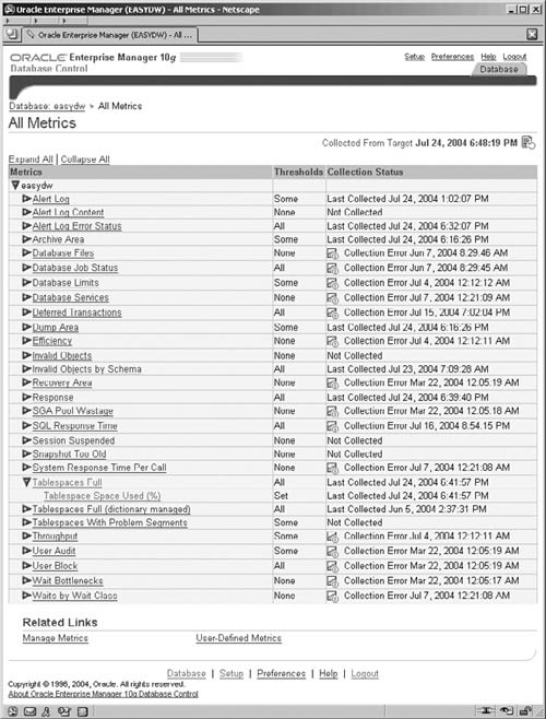
Clicking on the + icon to the right of the Tablespace Full metric expands the category to show the space used by the metric. From here you can drill down further to values collected and thresholds set for each tablespace and even further to displays and values for each tablespace.
When the tablespace full warning or critical thresholds are crossed, an alert will be generated and displayed in the Alert section on the database Home page. Notification mechanisms can also be defined by email or by paging the DBA on duty to correct this issue.
Summarized here are several features and enhancements in the database that simplify space management. Some of these features are outside the scope of this book, but we have listed the relevant chapters where we discuss certain features in more detail.
Locally managed tablespaces eliminate the need for periodically reorganizing tablespaces to reclaim fragmented space.
Tablespaces can be created with the SEGMENT SPACE MANAGEMENT AUTO clause to automate the management of free space inside a database segment, such as a table or index.
Automatic undo management eliminates the need to manage rollback segments manually.
As discussed in Chapter 3, Oracle Managed Files (OMF) can be used to create and delete files, as they are needed for the datafiles, on-line logs, and control files, eliminating the need to directly manage the files. All you need to do is specify the location of where you would like the files stored.
The Flash Recovery Area is new in Oracle Database 10g and is an area on disk that is used to contain database backups stored to disk, as well as for a new type of log file, called flashback logs. When the Flash Recovery Area is configured, the Oracle database will automatically manage the disk space utilization. The Flash Recovery Area is discussed in more detail in Chapter 12, and the flashback feature in Chapter 17.
Long-running operations that update or add new data to the database can fail when they run out of space. Reexecuting the procedure could take a long time, particularly if it was almost complete when it failed. A feature introduced in Oracle 9i, resumable statements, makes it possible to intervene and correct errors in the middle of an operation. When the problem that caused the failure is fixed, the operation is automatically resumed.
A resumable statement is suspended when one of the following errors occurs:
Out of space
Maximum extents reached
User space quota exceeded
The following operations are resumable:
SELECT statements that run out of temporary space (for sort areas)
DML statements—INSERT, UPDATE, and DELETE
Import/Export
SQL*Loader
DDL statements—CREATE TABLE ... AS SELECT, CREATE INDEX, ALTER INDEX ... REBUILD, ALTER TABLE ... MOVE PARTITION,
ALTER TABLE ... SPLIT PARTITION, ALTER INDEX ... REBUILD PARTITION, ALTER INDEX ... SPLIT PARTITION, CREATE MATERIALIZED VIEW, and CREATE MATERIALIZED VIEW LOG
Resumable mode must be enabled for a session. Optionally, you can specify a time-out period. If the error condition is not fixed within that time period, it will abort. You can also specify a name, which can help identify the session that has been suspended in the USER_RESUMABLE or DBA_RESUMABLE views. The following statement sets the time-out period for 3,600 seconds, or one hour, and assigns the name data warehouse load to resumable statements for the session.
SQL> ALTER SESSION
   ENABLE RESUMABLE
   TIMEOUT 3600 NAME 'data warehouse load';
SQL*Loader and the Import and Export utilities provide the same options as command-line parameters.
When a resumable statement is suspended, the error is reported in the alert log. The system also internally generates an AFTER SUSPEND system event. Users can register triggers for this event at both the database and schema level. The triggers can be used to notify the DBA when a statement is suspended, so corrective action can be taken.
Information about the status of resumable statements can be seen by looking at the DBA_RESUMABLE or USER_RESUMABLE views, as shown in the following example. The data warehouse load was suspended, because there was inadequate space to extend the PURCHASE_ PRODUCT_INDEX.
SQL> SELECT STATUS, TIMEOUT, START_TIME,
       SUSPEND_TIME, NAME, ERROR_MSG
FROM DBA_RESUMABLE

STATUS    TIMEOUT START_TIME        SUSPEND_TIME       NAME
--------- ------- ----------------- ------------------ --------
SUSPENDED 3600    08/16/04 06:27:56 08/16/04 14:01:05  data
warehouse load

ERROR_MSG
---------
ORA-01683: unable to extend index EASYDW.PURCHASE_PRODUCT_INDEX
partition PURCHASES_JUL04 by 2 in tablespace INDX
When a statement is suspended the session invoking the statement is put into a wait state. A row is inserted into the V$SESSION_WAIT as seen in the following example.
SQL> SELECT EVENT, STATE FROM V$SESSION_WAIT;

EVENT                                           STATE
----------------------------------------------- --------------
statement suspended, wait error to be cleared   WAITING
When space is added, the session will automatically resume. If space is not added within the time-out period, an error will occur.
We have already seen a number of management tasks. The ones specified here are by no means an exhaustive list, and there may very well be ones that are not mentioned here that may be applicable in your environment. There are also some additional tasks that you may want to consider.
When you suggest the construction of a test system, it is not uncommon for many people to throw their hands up in the air and say, “impossible.” But you should stop for a moment and consider the implication on your business if you don’t have a test system. When a test system exists, it can be used for a variety of reasons, such as:
Testing new software releases
Timing data loads
Evaluating management task times
Practicing management tasks
Testing scripts before executing in production
Assessing impact of maintenance tasks (e.g., index rebuild)
Determining query response times
Many people think that a test system has to be identical to the production system, but, in a warehouse, that is usually impossible. Therefore, what is required is a scaled-down version of the warehouse that is representative of the real warehouse. Ideally, numbers obtained from it should scale easily so that you can determine what the effect would be on your production warehouse.
Data inside the warehouse should, whenever possible, be representative of the real data. It may be that, to obtain the desired effect, you may have to extract data from the real warehouse and then load it into the test warehouse.
The various uses for a test system will now be discussed.
Once a database becomes a critical component in the business, and the information supplied from it is used to make critical business decisions, no one wants to jeopardize the business by introducing new software that may have problems. Therefore, if you have a test system, you can check that all of the important parts of the database software that you use are the same. The range of items to test could be extensive. For example, you will want to check that queries use the same optimizer strategy as before. If they have changed, then you should create outlines to ensure consistency of query response times.
However, you should always ensure, when using outlines, that performance will not degrade when a new version of Oracle is installed; it could improve due to an optimizer change, so always check for the current strategy.
Another important check to make is that key features that you rely on still function the same. For example, if you rely heavily on partition operations to maintain the data in your warehouse, then check that they still work.
Utilities you rely on should also be checked to see that no changes have occurred that cause them to change their behavior.
If a script is created that contains all of these important tasks, then each time you upgrade the software, you have only to run the scripts and check the results. Therefore, considerable effort will be required to construct the scripts the first time. Once completed, however, they can be run repeatedly and you will know that everything that is important to your environment will have been checked.
The test system provides an ideal opportunity to determine the load time for data and to practice any data cleansing that may be required. Generally, the fastest way to load data into an Oracle 9 i data warehouse is by using the utility SQL*Loader via the direct path method. But, you may want to compare the performance with external tables, particularly if you also need to perform transformations.
Now is also an ideal opportunity to practice and try out all of those management tasks before they are done in production. When it comes to testing backup and recovery processes, using very small databases initially and then moving on to the full size once you are sure that all of the procedures are working correctly will save time.
The test system provides an ideal opportunity to see the data warehouse in use before all the users are given access. Even with a limited user audience, you will be surprised that you will find queries that do not perform well.
Therefore, you now have time to diagnose the cause of the poor performance and resolve the problem by adding a new index, for example, or creating a materialized view to make the query perform faster.
In a test environment, it is unlikely that you will see an exact reproduction of usage of the data warehouse. Nevertheless, problems will still surface and it is easier to fix them now before the pressure comes with users demanding reports yesterday!
In this chapter, we have taken a look at some of the tasks required to manage a warehouse, examined many of the new features available in Oracle Database 10g to help with this, and used Oracle Enterprise Manager to simplify management of our warehouse. Ongoing tasks, including monitoring space usage, were discussed, and techniques for periodic reorganization using partition maintenance operations and on-line redefinition were introduced. Developing a test system and a business continuity plan are important considerations.
Hopefully, you can begin to appreciate what is involved in managing a database. Many of the tasks described here apply equally to a traditional OLTP database. It’s often the size of the data warehouse that makes the task different. Remember that it is better to manage now than not at all. Even something as simple as failing to monitor space usage could have disastrous results, usually when you can least afford the time to correct them.