
6.2.4 BICM Decoder
The decoding metric in (6.129) for the BICM decoder is defined in (3.22), and thus,
where
The PEP in (6.139) is then calculated as
where ![]() are the random variables modeling the L-values
are the random variables modeling the L-values ![]() ,
, ![]() was expressed as
was expressed as ![]() , and where, because of the linearity of the code, the error codeword
, and where, because of the linearity of the code, the error codeword ![]() satisfies
satisfies ![]() .
.
For any ![]() such that
such that ![]() (i.e., when
(i.e., when ![]() ), the L-values
), the L-values ![]() do not affect the PEP calculation. Therefore, there are only
do not affect the PEP calculation. Therefore, there are only ![]() pairs
pairs ![]() that are relevant for the PEP calculation in (6.187), and the PEP depends solely on
that are relevant for the PEP calculation in (6.187), and the PEP depends solely on ![]() and
and ![]() . We can thus write
. We can thus write
where
and where ![]() and
and ![]() ,
, ![]() are reindexed versions of
are reindexed versions of ![]() , and
, and ![]() , respectively. The reindexing enumerates only the elements with indices
, respectively. The reindexing enumerates only the elements with indices ![]() for which
for which ![]() , i.e., when
, i.e., when ![]() .
.
Moreover, knowing that the bits ![]() are an interleaved version of the bits
are an interleaved version of the bits ![]() and the L-values
and the L-values ![]() are obtained via deinterleaving of
are obtained via deinterleaving of ![]() , we can write
, we can write
where ![]() and
and ![]() are the interleaved/deinterleaved versions of
are the interleaved/deinterleaved versions of ![]() and
and ![]() , respectively.
, respectively.
The main reason to use (6.192) instead of (6.191) is that we already know how to model the L-values ![]() (see Chapter 5). We now have to address the more delicate issue of the joint probabilistic model of the L-values
(see Chapter 5). We now have to address the more delicate issue of the joint probabilistic model of the L-values ![]() . The situation which is the simplest to analyze occurs when the L-values
. The situation which is the simplest to analyze occurs when the L-values ![]() are independent, which we illustrate in Fig. 6.13 (a). In this case, the L-values
are independent, which we illustrate in Fig. 6.13 (a). In this case, the L-values ![]() are obtained from
are obtained from ![]() different channel outcomes
different channel outcomes ![]() . A more complicated situation to deal with arises when we can find at least two indices
. A more complicated situation to deal with arises when we can find at least two indices ![]() such that
such that ![]() and
and ![]() correspond to
correspond to ![]() and
and ![]() , i.e., when
, i.e., when ![]() and
and ![]() are L-values calculated at the same time
are L-values calculated at the same time ![]() (and thus, they are dependent). The case when the L-values are independent as well as the requirements on the interleaver for this assumption to hold are discussed below. The case where the L-values are not independent is discussed in Chapter 9.
(and thus, they are dependent). The case when the L-values are independent as well as the requirements on the interleaver for this assumption to hold are discussed below. The case where the L-values are not independent is discussed in Chapter 9.
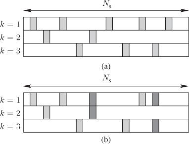
Figure 6.13 Codewords  corresponding to different interleaved error codewords
  . The L-values
  in (6.192) (indicated by rectangles) are (a) independent or (b) dependent random variables. The L-values, which are calculated using the same
  , i.e., at the same time
  , are indicated with dark-gray rectangles
In what follows we provide a lemma that will simplify the discussions thereafter.
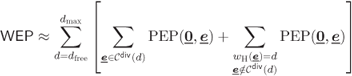
Lemma 6.17 allows us to simplify the WEP expression in (6.141) as follows:


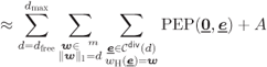
where the approximation in (6.208) follows from the truncation we make in the number of Hamming weights (HWs) to consider (![]() ). To transform (6.208) into a more suitable form we use a simple observation given by the following lemma.
). To transform (6.208) into a more suitable form we use a simple observation given by the following lemma.
To illustrate the result of Lemma 6.18 we show in Fig. 6.14 two error codewords ![]() with the same HW
with the same HW ![]() interleaved into codewords with different GHWs
interleaved into codewords with different GHWs ![]() .
.

Figure 6.14 The codewords  with the same HW
  are interleaved into codewords with different GHWs
  : (a) GHW
  and (b) GHW
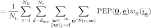
We now develop (6.208) as

where (6.214) follows from (6.209) and the third condition of the quasirandom interleaver in Definition 2.46, and where

The condition of having the spectrum ![]() bounded for given
bounded for given ![]() and growing
and growing ![]() is satisfied for turbo codes (TCs) (in fact, for TCs
is satisfied for turbo codes (TCs) (in fact, for TCs ![]() actually decreases with
actually decreases with ![]() ). On the other hand, for convolutional codes (CCs), the spectrum
). On the other hand, for convolutional codes (CCs), the spectrum ![]() may increase with
may increase with ![]() , but as discussed in Section 6.2.5, we may still neglect the effect of
, but as discussed in Section 6.2.5, we may still neglect the effect of ![]() for high SNR and large
for high SNR and large ![]() . Thus, to streamline further discussions, from now on we do not consider
. Thus, to streamline further discussions, from now on we do not consider ![]() in (6.214). Furthermore, if we assume the first condition of quasirandomness in Definition 2.46 to be satisfied, we can express (6.214) as
in (6.214). Furthermore, if we assume the first condition of quasirandomness in Definition 2.46 to be satisfied, we can express (6.214) as

Using steps similar to those that lead to (6.208) and then to (6.214), we can develop (6.144) as follows:


where ![]() in (6.220) is the input sequence corresponding to the codeword
in (6.220) is the input sequence corresponding to the codeword ![]() ,
, ![]() is the generalized input–output distance spectrum (GIODS) (see Definition 2.37), and to pass from (6.222) to (6.223) we used (2.114).
is the generalized input–output distance spectrum (GIODS) (see Definition 2.37), and to pass from (6.222) to (6.223) we used (2.114).
We note that (6.218) and (6.223) hold for any interleaver that satisfies the first and the third conditions in Definition 2.46. The second condition of quasirandomness is not exploited yet and, as we show in the following theorem, it simplifies the analysis further.
The key difference between the bounds for the ML decoder in (6.169) and (6.171) with those for the BICM decoder in (6.224) and (6.225), is that the performance of BICM depends on the DS of the binary code ![]() , and not on the DS of the code
, and not on the DS of the code ![]() . Further, because of the numerous approximations we made, the expressions (6.224) and (6.225) are not true bounds, but only approximations. Nevertheless, we will later show that these approximations indeed give accurate predictions of the WEP and BEP for BICM.
. Further, because of the numerous approximations we made, the expressions (6.224) and (6.225) are not true bounds, but only approximations. Nevertheless, we will later show that these approximations indeed give accurate predictions of the WEP and BEP for BICM.
The somewhat lengthy derivations above may be simplified using the model of independent and random assignment of the bits ![]() to the positions of the mapper in Fig. 2.24, and assuming that all codewords achieve their maximum diversity. Then,
to the positions of the mapper in Fig. 2.24, and assuming that all codewords achieve their maximum diversity. Then, ![]() is immediately obtained as the average of the PDF of the L-values over the different bit positions. Our objective here was to show that, in order to use such a random-assignment model, the interleaver (which is a deterministic element of the transceiver) must comply with all conditions of the quasirandomness in Definition 2.46.
is immediately obtained as the average of the PDF of the L-values over the different bit positions. Our objective here was to show that, in order to use such a random-assignment model, the interleaver (which is a deterministic element of the transceiver) must comply with all conditions of the quasirandomness in Definition 2.46.
The quasirandomness condition is not automatically satisfied by all interleavers. For example, we showed in Example 2.47 that for a convolutional code (CC), a rectangular interleaver does not satisfy the second condition of quasirandomness, which allowed us to replace ![]() by
by ![]() in (6.228). Therefore, while the first and the third condition of the quasirandomness hold for the rectangular interleaver and we may apply(6.218),10 we cannot use Theorem 6.20 in this case. The importance of the second condition of the quasirandomness is illustrated in the following example.
in (6.228). Therefore, while the first and the third condition of the quasirandomness hold for the rectangular interleaver and we may apply(6.218),10 we cannot use Theorem 6.20 in this case. The importance of the second condition of the quasirandomness is illustrated in the following example.

Figure 6.15 The analytical bound obtained using (6.225) and (6.236) (solid line) and the simulation results (markers) for pseudorandom and rectangular interleavers
For the remainder of this chapter, we use only pseudorandom interleavers, and thus, assume the conditions of quasirandomness in Definition 2.46 are fulfilled. In analogy to Example 6.15, the following example shows the performance of BICM with CENCs.
The IWD of the CENC ![]() in (6.245) is the total HW of all input sequences that generate error events with HW
in (6.245) is the total HW of all input sequences that generate error events with HW ![]() , where an error event is defined as a path in the trellis representation of the code that leaves the zero state and remerges with it after an arbitrary number of trellis stages. In the following example, we show how to calculate this IWD.
, where an error event is defined as a path in the trellis representation of the code that leaves the zero state and remerges with it after an arbitrary number of trellis stages. In the following example, we show how to calculate this IWD.

Figure 6.16 CENC  : (a) encoder and (b) state machine
We note that the enumeration of the diverging and merging paths in the trellis we analyzed in Example 6.23 does not consider all the codewords with HW ![]() because we do not take into account paths that diverged/merged multiple times. Assigning a codeword
because we do not take into account paths that diverged/merged multiple times. Assigning a codeword ![]() to the
to the ![]() th diverging/merging path, we see that all error codewords are mutually orthogonal and their sum
th diverging/merging path, we see that all error codewords are mutually orthogonal and their sum ![]() is also a validcodeword. Thus, they comply with the conditions we defined in Section 6.2.2, which lets us expurgate the codeword
is also a validcodeword. Thus, they comply with the conditions we defined in Section 6.2.2, which lets us expurgate the codeword ![]() from the bound. In other words, the enumeration of the uniquely-diverging codewords provides us with an expurgated bound. Therefore, for CENCs we have
from the bound. In other words, the enumeration of the uniquely-diverging codewords provides us with an expurgated bound. Therefore, for CENCs we have
where the approximation is due to the expurgation.
Since the performance of the receiver is directly affected by the characteristics of the CENC (via ![]() and
and ![]() ), efforts should be made to optimize the CENC. In fact, the CENCs we show in Table 2.1 are the encoders optimal in terms of the IWD
), efforts should be made to optimize the CENC. In fact, the CENCs we show in Table 2.1 are the encoders optimal in terms of the IWD ![]() . To find them, an exhaustive search over the CENC universe
. To find them, an exhaustive search over the CENC universe ![]() is performed: first, the free Hamming distance (FHD)
is performed: first, the free Hamming distance (FHD) ![]() is maximized and next, the corresponding term
is maximized and next, the corresponding term ![]() is minimized. If multiple encoders with the same
is minimized. If multiple encoders with the same ![]() and the same
and the same ![]() are found, those that minimize
are found, those that minimize ![]() are chosen, then
are chosen, then ![]() is analyzed, and so on. We refer to these optimized CENCs shown in Table 2.1 as “ODS CENCs” even if the literature uses the name “ODS codes.” We use the name ODS CENCs because
is analyzed, and so on. We refer to these optimized CENCs shown in Table 2.1 as “ODS CENCs” even if the literature uses the name “ODS codes.” We use the name ODS CENCs because ![]() depends on the encoder and not only on the code.
depends on the encoder and not only on the code.

Figure 6.17 Simulation results (circles) are compared to the bounds (6.263) and (6.266) (solid lines) and the approximations (6.244) and (6.242) for the ODS CENC with  ; the WEP results are shown for two values of
  . The bounds and approximations are only shown in the range of SNR where (6.259) is guaranteed to converge, i.e., for
6.2.5 BICM Decoder Revisited
To obtain the results in Theorem 6.20, we removed from (6.214) the contributions of the codewords that do not achieve their maximum diversity. Here, we want to have another look at this issue, but instead of proofs, we outline a few assumptions that hold indeed in practice and are sufficient to explain why we can neglect the factor ![]() in (6.214).
in (6.214).
To explicitly show the dependence of the PEP on the SNR, we use ![]() to denote the PEP in (6.226),
to denote the PEP in (6.226), ![]() to denote the PEP in (6.193), and
to denote the PEP in (6.193), and ![]() to denote (6.210).
to denote (6.210).
We then assume that ![]() is monotonically decreasing in both arguments, i.e.,
is monotonically decreasing in both arguments, i.e.,
In other words, we assert that increasing the HD between the codewords or increasing the SNR decreases the PEP.
Now we are able to relate (6.268) to the PEP expression ![]() . In general,
. In general, ![]() , but because
, but because ![]() is finite, for any
is finite, for any ![]() and
and ![]() , and thanks to (6.268), we can always find
, and thanks to (6.268), we can always find ![]() such that
such that
where ![]() .
.
Further, we assume that if ![]() is a “subcodeword” of
is a “subcodeword” of ![]() ,12 i.e.,
,12 i.e., ![]() , and
, and ![]() is such that it achieves its maximum diversity, i.e.,
is such that it achieves its maximum diversity, i.e., ![]() , then
, then
where ![]() and where (6.270) holds for any
and where (6.270) holds for any ![]() and any
and any ![]() .
.
Since ![]() , where
, where ![]() is the sum of L-values corresponding to the
is the sum of L-values corresponding to the ![]() nonzero bits in
nonzero bits in ![]() , to obtain
, to obtain ![]() we may need to remove some elements from
we may need to remove some elements from ![]() . Thus, the expression in (6.270) shows that removing one (or more) L-values from the sum
. Thus, the expression in (6.270) shows that removing one (or more) L-values from the sum ![]() yields a larger PEP. The intuition behind such an assertion is the following: each L-value contributes to improve the reliability of the detection so removing any element should produce a larger PEP. When the sum
yields a larger PEP. The intuition behind such an assertion is the following: each L-value contributes to improve the reliability of the detection so removing any element should produce a larger PEP. When the sum ![]() is composed of i.i.d. L-vales
is composed of i.i.d. L-vales ![]() , this can be better understood from Sections 6.3.3 and 6.3.4, where we showed that an upper bound on the PEP is determined by the exponential of the sum of the cumulant-generating functions (CGFs) corresponding to each of the L-values. As the CGFs are negative, removing one L-value corresponds to increasing the bound. On the other hand, if some of the L-values in
, this can be better understood from Sections 6.3.3 and 6.3.4, where we showed that an upper bound on the PEP is determined by the exponential of the sum of the cumulant-generating functions (CGFs) corresponding to each of the L-values. As the CGFs are negative, removing one L-value corresponds to increasing the bound. On the other hand, if some of the L-values in ![]() are not i.i.d., our assertion is slightly less obvious. We treat such a case in more detail in Chapter 9, where we show that adding dependent L-values decreases the PEP, and thus, removing L-values from the sum must increase the PEP.
are not i.i.d., our assertion is slightly less obvious. We treat such a case in more detail in Chapter 9, where we show that adding dependent L-values decreases the PEP, and thus, removing L-values from the sum must increase the PEP.
Combining (6.270) and (6.269) we have that for any ![]() and
and ![]() , we can find
, we can find ![]() such that
such that
where ![]() and where we used the fact that we can always find a codeword
and where we used the fact that we can always find a codeword ![]() with interleaving diversity
with interleaving diversity ![]() satisfying
satisfying ![]() (see (2.116)).
(see (2.116)).
We further make a simple extension to the conditions of quasirandomness we introduced in Section 2.7. Namely, we assume that if the interleaver is quasirandom, then the diversity efficiency ![]() decreases monotonically with
decreases monotonically with ![]() , i.e.,
, i.e.,
This property holds for random interleavers as we showed in (2.127). Here we extend it to the case of quasirandom (but fixed) interleavers, as we already did with other properties of the interleavers in Definition 2.46.
Let us recall now the formula for the WEP given by (6.224), where we reconsider the term ![]() in (6.215). Then, the WEP can be expressed as
in (6.215). Then, the WEP can be expressed as
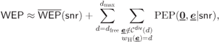
where
denotes the WEP approximation in (6.224), which ignores the codewords that do not achieve maximum diversity.
The WEP in (6.276) can be expressed as
where ![]() . In order to obtain (6.278) we used (6.271) and to obtain (6.279) we used (2.117). To obtain (6.280) we used (6.267) and (6.268), where
. In order to obtain (6.278) we used (6.271) and to obtain (6.279) we used (2.117). To obtain (6.280) we used (6.267) and (6.268), where ![]() should be sufficiently small so as to compensate for the increase of the first argument of the PEP (from
should be sufficiently small so as to compensate for the increase of the first argument of the PEP (from ![]() to
to ![]() ). Here we also used (6.275), which implies that
). Here we also used (6.275), which implies that ![]() .
.
From (6.281) we conclude that for sufficiently high SNR, we can neglect the term ![]() provided that we increase
provided that we increase ![]() so as to make the term
so as to make the term ![]() sufficiently small. This condition is fulfilled when using quasirandom interleavers. An alternative interpretation of this result is that the true WEP for a finite
sufficiently small. This condition is fulfilled when using quasirandom interleavers. An alternative interpretation of this result is that the true WEP for a finite ![]() is formed by two terms, where the second term
is formed by two terms, where the second term ![]() corresponds to a WEP obtained for an equivalent SNR
corresponds to a WEP obtained for an equivalent SNR ![]() . This factor might be relevant for the evaluation of the WEP for small values of
. This factor might be relevant for the evaluation of the WEP for small values of ![]() .
.
It is worth noting that all the considerations in this section may be repeated in the case of a BEP analysis, as well as for fading channels. For the former, the PEP should be weighted by the number of bits in error, and for the latter, ![]() should be replaced by
should be replaced by ![]() .
.