
Chapter 4
Information-Theoretic Elements
Information theory provides us with fundamental limits on the transmission rates supported by a channel. In this chapter, we analyze these limits for the coded modulation (CM) schemes presented in Chapter 2, paying special attention to bit-interleaved coded modulation (BICM).
This chapter is structured as follows. In Section 4.1, we introduce the concepts of mutual information (MI) and channel capacity; in Section 4.2, we study the maximum transmission rates for general CM systems; and in Section 4.3, for BICM systems. We review their relation and we analyze how they are affected by the choice of the (discrete) constellation. We pay special attention to the selection of the binary labeling and use of probabilistic shaping in BICM. We conclude the chapter by showing in Section 4.5 ready-to-use numerical quadrature formulas to efficiently compute MIs.
4.1 Mutual Information and Channel Capacity
We analyze the transmission model defined by (2.27), i.e., ![]() , where
, where ![]() is an
is an ![]() -dimensional zero-mean Gaussian vector with covariance matrix
-dimensional zero-mean Gaussian vector with covariance matrix ![]() . In this chapter, we are mostly interested in discrete constellations. However, we will initially assume that the input symbols
. In this chapter, we are mostly interested in discrete constellations. However, we will initially assume that the input symbols ![]() are modeled as independent and identically distributed (i.i.d.) continuous random variables characterized by their probability density function (PDF)
are modeled as independent and identically distributed (i.i.d.) continuous random variables characterized by their probability density function (PDF) ![]() . Considering constellations with continuous support (
. Considering constellations with continuous support (![]() ) provides us with an upper limit on the performance of discrete constellations. As mentioned before, we also assume that the channel state
) provides us with an upper limit on the performance of discrete constellations. As mentioned before, we also assume that the channel state ![]() is known at the receiver (through perfect channel estimation) and is not available at the transmitter. The assumption of the transmitter not knowing the channel state is important when analyzing the channel capacity (defined below) for fading channels.
is known at the receiver (through perfect channel estimation) and is not available at the transmitter. The assumption of the transmitter not knowing the channel state is important when analyzing the channel capacity (defined below) for fading channels.
The MI between the random vectors ![]() and
and ![]() conditioned on the channel state
conditioned on the channel state ![]() is denoted by
is denoted by ![]() and given by1
and given by1
where ![]() is given by (2.28).
is given by (2.28).
For future use, we also define the conditional MIs
Although ![]() is the most common notation for MI found in the literature (which we also used in Chapter 1), throughout this chapter, we also use an alternative notation
is the most common notation for MI found in the literature (which we also used in Chapter 1), throughout this chapter, we also use an alternative notation
which shows that conditioning on ![]() in (4.1) is equivalent to conditioning on the instantaneous signal-to-noise ratio (SNR); this notation also emphasizes the dependence of the MI on the input PDF
in (4.1) is equivalent to conditioning on the instantaneous signal-to-noise ratio (SNR); this notation also emphasizes the dependence of the MI on the input PDF ![]() . This notation allows us to express the MI for a fast fading channel (see Section 2.4) by averaging the MI in (4.5) over the SNR, i.e.,
. This notation allows us to express the MI for a fast fading channel (see Section 2.4) by averaging the MI in (4.5) over the SNR, i.e.,
where ![]() is given by (4.5). Throughout this chapter, we use the notation
is given by (4.5). Throughout this chapter, we use the notation ![]() and
and ![]() to denote MIs for the additive white Gaussian noise (AWGN) and fading channels, respectively.
to denote MIs for the additive white Gaussian noise (AWGN) and fading channels, respectively.
The MIs above have units of ![]() (or equivalently
(or equivalently ![]() ) and they define the maximum transmission rates that can be reliably2 used when the codewords
) and they define the maximum transmission rates that can be reliably2 used when the codewords ![]() are symbols generated randomly according to the continuous distribution PDF
are symbols generated randomly according to the continuous distribution PDF ![]() . More precisely, the converse of Shannon's channel coding theorem states that it is not possible to transmit information reliably above the MI, i.e.,
. More precisely, the converse of Shannon's channel coding theorem states that it is not possible to transmit information reliably above the MI, i.e.,
The channel capacity of a continuous-input continuous-output memoryless channel under average power constraint is defined as the maximum MI, i.e.,
where the optimization is carried out over all input distributions that satisfy the average energy constraint ![]() . Furthermore, we note that
. Furthermore, we note that ![]() is independent of
is independent of ![]() because we assumed that the transmitter does not know the channel. Because of this, we do not consider the case when the transmitter, knowing the channel, adjusts the signal's energy to the channel state.
because we assumed that the transmitter does not know the channel. Because of this, we do not consider the case when the transmitter, knowing the channel, adjusts the signal's energy to the channel state.
MI curves are typically plotted versus SNR, however, to better appreciate their behavior at low SNR, plotting MI versus the average information bit energy-to-noise ratio ![]() is preferred. To do this, first note that (4.7) can be expressed using (2.38) as
is preferred. To do this, first note that (4.7) can be expressed using (2.38) as
The notation ![]() emphasizes that the MI is a function of both
emphasizes that the MI is a function of both ![]() and
and ![]() , which will be useful throughout this chapter. In what follows, however, we discuss
, which will be useful throughout this chapter. In what follows, however, we discuss ![]() as a function of
as a function of ![]() for a given input distribution, i.e.,
for a given input distribution, i.e., ![]() .
.
The MI is an increasing function of the SNR, and thus, it has an inverse, which we denote by ![]() . By using this inverse function (for any given
. By using this inverse function (for any given ![]() ) in both sides of (4.14), we obtain
) in both sides of (4.14), we obtain
Furthermore, by rearranging the terms, we obtain
which shows that ![]() is bounded from below by
is bounded from below by ![]() , which is a function of the rate
, which is a function of the rate ![]() .
.
In other words, the function ![]() in (4.16) gives, for a given input distribution
in (4.16) gives, for a given input distribution ![]() , a lower bound on the
, a lower bound on the ![]() needed for reliable transmission at rate
needed for reliable transmission at rate ![]() . For example, for the AWGN channel in Example 4.1, and by using (4.9) in (4.16), we obtain
. For example, for the AWGN channel in Example 4.1, and by using (4.9) in (4.16), we obtain
In this case, the function ![]() depends solely on
depends solely on ![]() (and not on
(and not on ![]() , as in (4.16)), which follows because
, as in (4.16)), which follows because ![]() in (4.9) depends only on
in (4.9) depends only on ![]() .
.
The expressions in (4.17) allow us to find a lower bound on ![]() when
when ![]() , or equivalently, when
, or equivalently, when ![]() , i.e., in the low-SNR regime. Using (4.17), we obtain
, i.e., in the low-SNR regime. Using (4.17), we obtain
which we refer to as the Shannon limit (SL). The bound in (4.18) corresponds to the minimum average information bit energy-to-noise ratio ![]() needed to reliably transmit information when
needed to reliably transmit information when ![]() .
.
For notation simplicity, in (4.14)–(4.16), we consider nonfading channels. It is important to note, however, that because ![]() , exactly the same expressions apply to fading channels, i.e., when
, exactly the same expressions apply to fading channels, i.e., when ![]() is replaced by
is replaced by ![]() .
.
4.2 Coded Modulation
In this section, we focus on the practically relevant case of discrete constellations, and thus, we restrict our analysis to probability mass functions (PMFs) ![]() with
with ![]() nonzero mass points, i.e.,
nonzero mass points, i.e., ![]() ,
, ![]() .
.
4.2.1 CM Mutual Information
We define the coded modulation mutual information (CM-MI) as the MI between the input and the output of the channel when a discrete constellation is used for transmission. As mentioned in Section 2.5.1, in this case, the transmitted symbols are fully determined by the PMF ![]() , and thus, we use the matrix
, and thus, we use the matrix ![]() to denote the support of the PMF (the constellation
to denote the support of the PMF (the constellation ![]() ) and the vector
) and the vector ![]() to denote the probabilities associated with the symbols (the input distribution). The CM-MI can be expressed using (4.2), where the first integral is replaced by a sum and the PDF
to denote the probabilities associated with the symbols (the input distribution). The CM-MI can be expressed using (4.2), where the first integral is replaced by a sum and the PDF ![]() by the PMF
by the PMF ![]() , i.e.,
, i.e.,
where the notation ![]() emphasizes the dependence of the MI on the input PMF
emphasizes the dependence of the MI on the input PMF ![]() (via
(via ![]() and
and ![]() , see (2.41)).
, see (2.41)).
For the AWGN channel with channel transition probability (2.31), the CM-MI in (4.21) can be expressed as
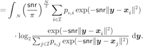
For a uniform input distribution ![]() in (2.42), the above expression particularizes to
in (2.42), the above expression particularizes to


Figure 4.1  PSK constellations and AWGN channel: (a) CM-MI and (b)
  in (4.16). The AWGN capacity
  and the corresponding
  are shown for reference

Figure 4.2  PAM constellations and AWGN channel: (a) CM-MI and (b)
  in (4.16). The AWGN capacity
  and the corresponding
  are shown for reference
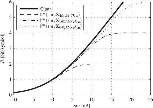
Figure 4.3 CM-MI for 4PSK (4QAM) and for the  QAM constellations in Fig. 2.11 (
 ) over the AWGN channel. The AWGN capacity
  in (4.9) is also shown

Figure 4.4  PAM constellations and Rayleigh fading channel: (a) CM-MI and (b)
 in (4.16). The average capacity
  and the corresponding
  are shown for reference
4.2.2 CM Capacity
The CM-MI ![]() corresponds to the maximum transmission rate when the codewords' symbols
corresponds to the maximum transmission rate when the codewords' symbols ![]() are taken from the constellation
are taken from the constellation ![]() following the PMF
following the PMF ![]() . In such cases, the role of the receiver is to find the transmitted codewords using
. In such cases, the role of the receiver is to find the transmitted codewords using ![]() by applying the maximum likelihood (ML) decoding rule we defined in Chapter 3. In practice, the CM encoder must be designed having the decoding complexity in mind. To ease the implementation of the ML decoder, particular encoding structures are adopted. This is the idea behind trellis-coded modulation (TCM) (see Fig. 2.4), where the convolutional encoder (CENC) generates symbols
by applying the maximum likelihood (ML) decoding rule we defined in Chapter 3. In practice, the CM encoder must be designed having the decoding complexity in mind. To ease the implementation of the ML decoder, particular encoding structures are adopted. This is the idea behind trellis-coded modulation (TCM) (see Fig. 2.4), where the convolutional encoder (CENC) generates symbols ![]() which are mapped directly to constellation symbols
which are mapped directly to constellation symbols ![]() . In this case, the code can be represented using a trellis structure, which means that the Viterbi algorithm can be used to implement the ML decoding rule, and thus, the decoding complexity is manageable.
. In this case, the code can be represented using a trellis structure, which means that the Viterbi algorithm can be used to implement the ML decoding rule, and thus, the decoding complexity is manageable.
The most popular CM schemes are based on uniformly distributed constellation points. However, using a uniform input distribution is not mandatory, and thus, one could think of using an arbitrary PMF (and/or a nonequally spaced constellation) so that the CM-MI is increased. To formalize this, and in analogy with (4.8), we define the CM capacity for a given constellation size ![]() as
as
where the optimization over ![]() and
and ![]() is equivalent to the optimization over the PMF
is equivalent to the optimization over the PMF ![]() .
.
The optimization problem in (4.25) is done under constraint ![]() , where
, where ![]() depends on both
depends on both ![]() and
and ![]() . In principle, a constraint
. In principle, a constraint ![]() could be imposed; however, for the channel in (2.27) we consider here, an increase in
could be imposed; however, for the channel in (2.27) we consider here, an increase in ![]() always results in a higher MI and thus, the constraint is always active.
always results in a higher MI and thus, the constraint is always active.
Again, the optimization result (4.25) should be interpreted as the maximum number of bits per symbol that can be reliably transmitted using a fully optimized ![]() -point constellation, i.e., when for each SNR value, the constellation and the input distribution are selected in order to maximize the CM-MI. This is usually referred to as signal shaping.
-point constellation, i.e., when for each SNR value, the constellation and the input distribution are selected in order to maximize the CM-MI. This is usually referred to as signal shaping.
The CM capacity for fading channels is defined as
We note that the optimal constellations ![]() and
and ![]() , i.e., those solving (4.25) or (4.26), are not the same for the AWGN and fading channels. This is different from the case of continuous distributions
, i.e., those solving (4.25) or (4.26), are not the same for the AWGN and fading channels. This is different from the case of continuous distributions ![]() , where the Gaussian distribution is optimal for each value of
, where the Gaussian distribution is optimal for each value of ![]() over the AWGN channel and thus, the same distribution yields the capacity of fading channels, cf. Example 4.2.
over the AWGN channel and thus, the same distribution yields the capacity of fading channels, cf. Example 4.2.
The joint optimization over both ![]() and
and ![]() is a difficult problem, and thus, one might prefer to solve simpler ones:
is a difficult problem, and thus, one might prefer to solve simpler ones:
The expression (4.28) is typically called geometrical shaping as only the constellation symbols (geometry) are being optimized, while the problem (4.27) is called probabilistic shaping as the probabilities of the constellation symbols are optimized.
Finally, as a pragmatic compromise between the fully optimized signal shaping of (4.25) and the geometric/probabilistic solutions of , we may optimize the distribution ![]() while maintaining the “structure” of the constellation, i.e., allowing for a scaling of a predefined constellation with a factor
while maintaining the “structure” of the constellation, i.e., allowing for a scaling of a predefined constellation with a factor ![]()
where ![]() is the optimal value of
is the optimal value of ![]() .
.

Figure 4.5 Solution of problem (4.27): optimal PMF for an equidistant 8PAM constellation in the AWGN channel

Figure 4.6 Solution of problem (4.28): optimal input distribution for an  -ary constellation in the AWGN channel

Figure 4.7 Solution of problem (4.29): optimal PMF for an equidistant 8PAM constellation in the AWGN channel
We conclude this section by quantifying the gains obtained by changing the input distribution. We show in Fig. 4.8 (a)3 the CM-MI ![]() (8PAM with a uniform input distribution), as well as
(8PAM with a uniform input distribution), as well as ![]() in (4.27),
in (4.27), ![]() in (4.28), and
in (4.28), and ![]() in (4.29). These results show that the gains offered by probabilistic and geometric shaping are quite small; however, when the mixed optimization in (4.29) is done (i.e., when the probability and the gain
in (4.29). These results show that the gains offered by probabilistic and geometric shaping are quite small; however, when the mixed optimization in (4.29) is done (i.e., when the probability and the gain ![]() are jointly optimized), the gap to the AWGN capacity is closed for any
are jointly optimized), the gap to the AWGN capacity is closed for any ![]() . To clearly observe this effect, we show in Fig. 4.8 (b) the MI gains offered (with respect to
. To clearly observe this effect, we show in Fig. 4.8 (b) the MI gains offered (with respect to ![]() ) by the two approaches as well as the gain offered by using the optimal (Gaussian) distribution. This figure shows that the optimization in (4.29) gives considerably larger gains, which are close to optimal ones for any
) by the two approaches as well as the gain offered by using the optimal (Gaussian) distribution. This figure shows that the optimization in (4.29) gives considerably larger gains, which are close to optimal ones for any ![]() .
.
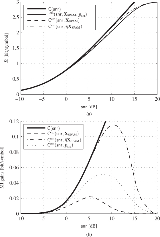
Figure 4.8 (a) The CM-MI  , the capacities
  in (4.27),
  in (4.28), and
  in (4.29) and (b) their respective MI gains with respect to
 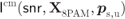 . The AWGN capacity (a) and the corresponding gain (b) are also shown
4.3 Bit-Interleaved Coded Modulation
In this section, we are interested in finding the rates that can be reliably used by the BICM transceivers shown in Fig. 2.7. We start by defining achievable rates for BICM transceivers with arbitrary input distributions, and we then move to study the problem of optimizing the system's parameters to increase these rates.
4.3.1 BICM Generalized Mutual Information
For the purpose of the discussion below, we rewrite here (3.23) as
where the symbol-decoding metric
is defined via the bit decoding metrics, each given by
The symbol-decoding metric ![]() is not proportional to
is not proportional to ![]() , i.e., the decoder does not implement the optimal ML decoding. To find achievable rates in this case, we consider the BICM decoder as the so-called mismatched decoder. In this context, for an arbitrary decoding metric
, i.e., the decoder does not implement the optimal ML decoding. To find achievable rates in this case, we consider the BICM decoder as the so-called mismatched decoder. In this context, for an arbitrary decoding metric ![]() , reliable communication is possible for rates below the generalized mutual information (GMI) between
, reliable communication is possible for rates below the generalized mutual information (GMI) between ![]() and
and ![]() , which is defined as
, which is defined as
where
We immediately note that if ![]() and
and ![]() , we obtain
, we obtain
that is, using symbol metrics matched to the conditional PDF of the channel output, we obtain the CM-MI ![]() in (4.23). This result is generalized in the following theorem.
in (4.23). This result is generalized in the following theorem.
The following theorem gives an expression for ![]() in (4.35) when the decoder uses a symbol metric
in (4.35) when the decoder uses a symbol metric ![]() given by (4.32) and an arbitrary bit metric
given by (4.32) and an arbitrary bit metric ![]() .
.
Corollary 4.12 shows that when the symbol metrics are constrained to follow (4.32), the best we can do is to use the bits metrics (4.33). The resulting achievable rates lead to the following definition of the BICM generalized mutual information (BICM-GMI) for fading and nonfading channels as
where the dependence on the constellation symbols ![]() , their labeling
, their labeling ![]() , and the bits' PMF
, and the bits' PMF ![]() is made explicit in the argument of
is made explicit in the argument of ![]() . The bitwise MIs necessary to calculate the BICM-GMI in (4.54), (4.55) are given by
. The bitwise MIs necessary to calculate the BICM-GMI in (4.54), (4.55) are given by
At this point, some observations are in order:
- The MI in (4.22) is an achievable rate for any CM transmission, provided that the receiver implements the ML decoding rule. The BICM-GMI in (4.54) and (4.55) is an achievable rate for the (suboptimal) BICM decoder.
- The BICM-GMI was originally derived without the notion of mismatched decoding, but based on an equivalent channel model where the interface between the interleaver and deinterleaver in Fig. 2.7 is replaced by
 parallel memoryless binary-input continuous-output (BICO)channels. Such a model requires the assumption of a quasi-random interleaver. Hence, the value of Theorem 4.11 is that it holds independently of the interleaver's presence.
 - No converse decoding theorem exists, i.e., while the BICM-GMI defines an achievable rate, it has not been proved to be the largest achievable rate when using a mismatched (BICM) decoder. This makes difficult a rigorous comparison of BICM transceivers because we cannot guarantee that differences in the BICM-GMI will translate into differences between the maximum achievable rates. However, practical coding schemes most often closely follow and do not exceed the BICM-GMI. This justifies its practical use as a design rule for the BICM. We illustrate this in the following example.

Figure 4.9 Throughputs  obtained for the AWGN channel and a PCCENC TENC with 11 different code rates
  for (a) 4PAM and (b) 8PAM labeled by the BRGC. The CM-MI, BICM-GMI, and AWGN capacity
  in (4.9) are also shown
While the quantities (4.54) and (4.55) were originally called the BICM capacity, we avoid using the term “capacity” to point out that no optimization of the input distribution is carried out. Using (4.56), the BICM-GMI in (4.54) can be expressed as
where to pass from (4.58) to (4.59) we used the law of total probability applied to expectations. Moreover, by using (2.75) and by expanding the expectation ![]() over
over ![]() and then over
and then over ![]() , we can express (4.59) as
, we can express (4.59) as


where to pass from (4.60) to (4.61), we used (2.75) and the fact that the value of ![]() does not affect the conditional channel transition probability, i.e.,
does not affect the conditional channel transition probability, i.e., ![]() . The dependence of the BICM-GMI on the labeling
. The dependence of the BICM-GMI on the labeling ![]() becomes evident because the sets
becomes evident because the sets ![]() appear in (4.61), and as we showed in Section 2.5.2, these sets define the subconstellations generated by the labeling.
appear in (4.61), and as we showed in Section 2.5.2, these sets define the subconstellations generated by the labeling.
For AWGN channels (![]() ), the BICM-GMI in (4.61) can be expressed as
), the BICM-GMI in (4.61) can be expressed as
Furthermore, for uniformly distributed bits, ![]() for
for ![]() , and thus, the BICM-GMI in (4.62) becomes
, and thus, the BICM-GMI in (4.62) becomes

where we use ![]() to denote uniformly distributed bits, i.e.,
to denote uniformly distributed bits, i.e., ![]() . In what follows, we show examples of the BICM-GMI for different constellations
. In what follows, we show examples of the BICM-GMI for different constellations ![]() and labelings
and labelings ![]() with uniform input distributions.
with uniform input distributions.

Figure 4.10 BICM-GMI and CM-MI for 8PSK and 16PSK (see Fig. 2.9) over the AWGN channel (a) and the corresponding functions  in (4.16) (b). The AWGN capacity
  in (4.9)
  (a) and the function
  in (4.17) together with the SL in (4.18) (b) are also shown

Figure 4.11 BICM-GMI and CM-MI for 8PAM over the AWGN channel (a) and the corresponding functions  in (4.16) (b). The BICM-GMI is shown for the four binary labelings in Fig. 2.13. The shadowed regions shows the inequalities (4.7) (a) and (4.16) (b) for the BSGC. The AWGN capacity
  in (4.9)
  (a) and the function
  in (4.17) together with the SL in (4.18) (b) are also shown

Figure 4.12 Functions  in (4.16) for the BICM-GMI for 4PSK and 8PSK over the AWGN channel and for all binary labelings that produce different BICM-GMI curves. The function
  in (4.17) and the SL in (4.18) are also shown