
Chapter 2
Preliminaries
In this chapter, we introduce the preliminaries for this book. In particular, we introduce all the building blocks of coded modulation (CM) and bit-interleaved coded modulation (BICM) transceivers. Although some chapters are more or less self-contained, reading this chapter before proceeding further is highly recommended. This chapter is organized as follows. We introduce the notation convention in Section 2.1 and in Section 2.2 we present a general model for the problem of binary transmission over a physical channel. Coded modulation systems are briefly analyzed in Section 2.3 and the channel models of interest are discussed in Section 2.4. In Section 2.5 constellations and binary labelings are discussed. Finally, in Section 2.6, we review some of the channel codes that will be used later in the book.
2.1 Notation Convention
We use lowercase letters ![]() to denote a scalar, boldface letters
to denote a scalar, boldface letters ![]() to denote a length-
to denote a length-![]() column vector; both can be indexed as
column vector; both can be indexed as ![]() and
and ![]() , where
, where ![]() denotes transposition. A sequence of scalars is denoted by a row vector
denotes transposition. A sequence of scalars is denoted by a row vector ![]() and a sequence of
and a sequence of ![]() -dimensional vectors by
-dimensional vectors by

where ![]() .
.
An ![]() matrix is denoted as
matrix is denoted as ![]() and its elements are denoted by
and its elements are denoted by ![]() where
where ![]() and
and ![]() . The all-zeros and the all-ones column vectors are denoted by
. The all-zeros and the all-ones column vectors are denoted by ![]() and
and ![]() , respectively. The sequences of such vectors are denoted by
, respectively. The sequences of such vectors are denoted by ![]() and
and ![]() , respectively. The identity matrix of size
, respectively. The identity matrix of size ![]() is denoted by
is denoted by ![]() . The inner product of two vectors
. The inner product of two vectors ![]() and
and ![]() is defined as
is defined as ![]() , the Euclidean norm of a length-
, the Euclidean norm of a length-![]() vector
vector ![]() is defined as
is defined as ![]() , and the
, and the ![]() (Manhattan) norm as
(Manhattan) norm as ![]() . The Euclidean norm of the sequence
. The Euclidean norm of the sequence ![]() in (2.1) is given by
in (2.1) is given by ![]() .
.
Sets are denoted using calligraphic letters ![]() , where
, where ![]() represents the Cartesian product between
represents the Cartesian product between ![]() and
and ![]() . The exception to this notation is used for the number sets. The real numbers are denoted by
. The exception to this notation is used for the number sets. The real numbers are denoted by ![]() , the nonnegative real numbers by
, the nonnegative real numbers by ![]() , the complex numbers by
, the complex numbers by ![]() , the natural numbers by
, the natural numbers by ![]() , the positive integers by
, the positive integers by ![]() , and the binary set by
, and the binary set by ![]() . The set of real matrices of size
. The set of real matrices of size ![]() (or–equivalently–of length-
(or–equivalently–of length-![]() sequences of
sequences of ![]() -dimensional vectors) is denoted by
-dimensional vectors) is denoted by ![]() ; the same notation is used for matrices and vector sequences of other types, e.g., binary
; the same notation is used for matrices and vector sequences of other types, e.g., binary ![]() or natural
or natural ![]() . The empty set is denoted by
. The empty set is denoted by ![]() . The negation of the bit
. The negation of the bit ![]() is denoted by
is denoted by ![]() .
.
An extension of the Cartesian product is the ordered direct product, which operates on vectors/matrices instead of sets. It is defined as
where ![]() for
for ![]() and
and ![]() .
.
The indicator function is defined as ![]() when the statement
when the statement ![]() is true and
is true and ![]() , otherwise. The natural logarithm is denoted by
, otherwise. The natural logarithm is denoted by ![]() and the base-2 logarithm by
and the base-2 logarithm by ![]() . The real part of a complex number
. The real part of a complex number ![]() is denoted by
is denoted by ![]() and its imaginary part by
and its imaginary part by ![]() , thus
, thus ![]() . The floor and ceiling functions are denoted by
. The floor and ceiling functions are denoted by ![]() and
and ![]() , respectively.
, respectively.
The Hamming distance (HD) between the binary vectors ![]() and
and ![]() is denoted by
is denoted by ![]() , the Hamming weight (HW) of the vector
, the Hamming weight (HW) of the vector ![]() by
by ![]() , which we generalize to the case of sequences of binary vectors
, which we generalize to the case of sequences of binary vectors ![]() as
as
i.e., the generalized Hamming weight (GHW) in (2.3) is the vector of HWs of each row of ![]() . Similarly, the total HD between the sequences of binary vectors
. Similarly, the total HD between the sequences of binary vectors ![]() is denoted by
is denoted by ![]() .
.
Random variables are denoted by capital letters ![]() , probabilities by
, probabilities by ![]() , and the cumulative distribution function (CDF) of
, and the cumulative distribution function (CDF) of ![]() by
by ![]() . The probability mass function (PMF) of the random vector
. The probability mass function (PMF) of the random vector ![]() is denoted by
is denoted by ![]() , the probability density function (PDF) of
, the probability density function (PDF) of ![]() by
by ![]() . The joint PDF of the random vectors
. The joint PDF of the random vectors ![]() and
and ![]() is denoted by
is denoted by ![]() and the PDF of
and the PDF of ![]() conditioned on
conditioned on ![]() by
by ![]() . The same notation applies to joint and conditional PMFs, i.e.,
. The same notation applies to joint and conditional PMFs, i.e., ![]() and
and ![]() . Note that the difference in notation between random vectors and matrices is subtle. The symbols for vectors are capital italic boldface while the symbols for matrices are not italic.
. Note that the difference in notation between random vectors and matrices is subtle. The symbols for vectors are capital italic boldface while the symbols for matrices are not italic.
The expectation of an arbitrary function ![]() over the joint distribution of
over the joint distribution of ![]() and
and ![]() is denoted by
is denoted by ![]() and the expectation over the conditional distribution is denoted by
and the expectation over the conditional distribution is denoted by ![]() . The unconditional and conditional variance of a scalar function
. The unconditional and conditional variance of a scalar function ![]() are respectively denoted as
are respectively denoted as
The moment-generating function (MGF) of the random variable ![]() is defined as
is defined as
where ![]() .
.
The notation ![]() is used to denote a Gaussian random variable with mean value
is used to denote a Gaussian random variable with mean value ![]() and variance
and variance ![]() ; its PDF is given by
; its PDF is given by
The complementary CDF of ![]() is defined as
is defined as
We also use the complementary error function defined as
If ![]() and
and ![]() , then
, then ![]() is a normalized bivariate Gaussian variable with correlation
is a normalized bivariate Gaussian variable with correlation ![]() . Its PDF is given by
. Its PDF is given by
and the complementary CDF by

The convolution of two functions ![]() and
and ![]() is denoted by
is denoted by ![]() and the
and the ![]() -fold self-convolution of
-fold self-convolution of ![]() is defined as
is defined as
For any function ![]() , we also define
, we also define
For any ![]() , with
, with ![]() and
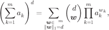
and ![]() , the multinomial coefficient defined as
, the multinomial coefficient defined as
can be interpreted as the number of all different partitions of ![]() elements into
elements into ![]() sets, where the partition is defined by the number of elements
sets, where the partition is defined by the number of elements ![]() in the
in the ![]() th set. In particular, we have
th set. In particular, we have

2.2 Linear Modulation
In this book, we deal with transmission of binary information over a physical medium (channel) using linear modulation. At the transmitter side, the sequence of independent and uniformly distributed (i.u.d.) bits ![]() is mapped (encoded) into a sequence of symbols
is mapped (encoded) into a sequence of symbols ![]() which is then used to alter the amplitude of a finite-energy real-valued waveform
which is then used to alter the amplitude of a finite-energy real-valued waveform ![]() which is sent over the channel. The whole transmitted waveform is then given by
which is sent over the channel. The whole transmitted waveform is then given by
where ![]() is the signaling rate, which is proportional to the bandwidth occupied by the transmitted signals. The transmission rate is defined as
is the signaling rate, which is proportional to the bandwidth occupied by the transmitted signals. The transmission rate is defined as
where
A general structure of such a system is schematically shown in Fig. 2.1.

Figure 2.1 A simplified block diagram of a digital transmitter—receiver pair
The channel introduces scaling via the channel gain ![]() and perturbations via the signal (noise)
and perturbations via the signal (noise) ![]() which models the unknown thermal noise (Johnson–Nyquist noise) introduced by electronic components in the receiver. The signal observed at the receiver is given by
which models the unknown thermal noise (Johnson–Nyquist noise) introduced by electronic components in the receiver. The signal observed at the receiver is given by
The general problem in communications is to guess (estimate) the transmitted bits ![]() using the channel observation
using the channel observation ![]() .
.
We assume that ![]() varies slowly compared to the duration of the waveform
varies slowly compared to the duration of the waveform ![]() , that the noise
, that the noise ![]() is a random white Gaussian process, and that the Nyquist condition for
is a random white Gaussian process, and that the Nyquist condition for ![]() is satisfied (i.e., for
is satisfied (i.e., for ![]() , we have:
, we have: ![]() if
if ![]() and
and ![]() if
if ![]() ). In this case, the receiver does not need to take into account the continuous-time signal
). In this case, the receiver does not need to take into account the continuous-time signal ![]() , but rather, only its filtered (via the so-called matched filter
, but rather, only its filtered (via the so-called matched filter ![]() ) and sampled version. Therefore, sampling the filtered output
) and sampled version. Therefore, sampling the filtered output ![]() at time instants
at time instants ![]() provides us with sufficient statistics to estimate the transmitted sequence
provides us with sufficient statistics to estimate the transmitted sequence ![]() . Moreover, by considering
. Moreover, by considering ![]() waveforms
waveforms ![]() that fulfill the Nyquist condition, we arrive at the
that fulfill the Nyquist condition, we arrive at the ![]() -dimensional discrete-time model
-dimensional discrete-time model
where ![]() and
and ![]() .
.
Using the model in (2.24), the channel and part of the transmitter and receiver in Fig. 2.1 are replaced by a discrete-time model, where the transmitted sequence of symbols is denoted by ![]() and
and ![]() is the sequence of real channel attenuations (gains) varying independently of
is the sequence of real channel attenuations (gains) varying independently of ![]() and assumed to be known (perfectly estimated) at the receiver. The transmitted sequence of symbols
and assumed to be known (perfectly estimated) at the receiver. The transmitted sequence of symbols ![]() is corrupted by additive noise
is corrupted by additive noise ![]() , as shown in Fig. 2.2.
, as shown in Fig. 2.2.

Figure 2.2 Simplified block diagram of the model in Fig. 2.1 where the continuous-time channel model is replaced by a discrete-time model
The main design challenge is now to find an encoder that maps the sequence of information bits ![]() to a sequence of vectors
to a sequence of vectors ![]() so that reliable transmission of the information bits with limited decoding complexity is guaranteed. Typically, each element in
so that reliable transmission of the information bits with limited decoding complexity is guaranteed. Typically, each element in ![]() belongs to a discrete constellation
belongs to a discrete constellation ![]() of size
of size ![]() . We assume
. We assume ![]() , which leads us to consider the output of the encoder as
, which leads us to consider the output of the encoder as ![]() -ary symbols represented by length-
-ary symbols represented by length-![]() vectors of bits
vectors of bits ![]() .
.
It is thus possible to consider that encoding is done in two steps: first a binary encoder (ENC) generates a sequence of ![]() code bits
code bits ![]() , and next, the code bits are mapped to constellation symbols. We will refer to the mapping between the information sequence
, and next, the code bits are mapped to constellation symbols. We will refer to the mapping between the information sequence ![]() and the symbol sequence
and the symbol sequence ![]() as CM encoding. This operation is shown in Fig. 2.3, where the mapper
as CM encoding. This operation is shown in Fig. 2.3, where the mapper ![]() is a one-to-one mapping between the length-
is a one-to-one mapping between the length-![]() binary vector
binary vector ![]() and the constellation symbols
and the constellation symbols ![]() , i.e.,
, i.e., ![]() . The modulation block is discussed in more detail in Section 2.5 and the encoding block in Section 2.6. At the receiver, the decoder will use maximum likelihood (ML) decoding, maximum a posteriori (MAP) decoding, or a BICM-type decoding; these are analyzed in Chapter 3.
. The modulation block is discussed in more detail in Section 2.5 and the encoding block in Section 2.6. At the receiver, the decoder will use maximum likelihood (ML) decoding, maximum a posteriori (MAP) decoding, or a BICM-type decoding; these are analyzed in Chapter 3.

Figure 2.3 A simplified block diagram of the model in Fig. 2.2. The CM encoder is composed of a encoder (ENC) and a mapper ( ). The CM decoder uses one of the rules defined in Chapter 3
The rate of the binary encoder (also known as the code rate) is given by
where ![]() , and thus,
, and thus,
The CM encoder in Fig. 2.2 maps each of the ![]() possible messages to the sequence
possible messages to the sequence ![]() . The code
. The code ![]() with
with ![]() is defined as the set of all codewords corresponding to the
is defined as the set of all codewords corresponding to the ![]() messages.1 Similarly, we use
messages.1 Similarly, we use ![]() to denote the binary code, i.e., the set of binary codewords
to denote the binary code, i.e., the set of binary codewords ![]() . Having defined
. Having defined ![]() , the sets
, the sets ![]() and
and ![]() are equivalent: the encoder is a one-to-one function that assigns each information message
are equivalent: the encoder is a one-to-one function that assigns each information message ![]() to one of the
to one of the ![]() possible symbol sequences
possible symbol sequences ![]() , or equivalently, to one of the corresponding bit sequences
, or equivalently, to one of the corresponding bit sequences ![]() . At the receiver's side, the decoder uses the vector of observations
. At the receiver's side, the decoder uses the vector of observations ![]() to generate an estimate of the information sequence
to generate an estimate of the information sequence ![]() .
.
In the following section, we briefly review three popular ways of implementing the encoder–decoder pair in Fig. 2.2 or 2.3.
2.3 Coded Modulation
We use the name coded modulation to refer to transceivers where ![]() . In what follows we briefly describe popular ways of implementing such systems.
. In what follows we briefly describe popular ways of implementing such systems.
2.3.1 Trellis-Coded Modulation
Ungerboeck proposed trellis-coded modulation (TCM) in 1982 as a way of combining convolutional encoders (CENCs) (very popular at that time) with ![]() -ary constellations. Targeting transmission over nonfading channels, TCM aimed at increasing the Euclidean distance (ED) between the transmitted codewords. In order to maximize the ED, the encoder and the mapper
-ary constellations. Targeting transmission over nonfading channels, TCM aimed at increasing the Euclidean distance (ED) between the transmitted codewords. In order to maximize the ED, the encoder and the mapper ![]() are jointly designed; Ungerboeck proposed a design strategy based on the so-called labeling by set-partitioning (SP) and showed gains are attainable for various CENCs.
are jointly designed; Ungerboeck proposed a design strategy based on the so-called labeling by set-partitioning (SP) and showed gains are attainable for various CENCs.
A typical TCM structure is shown in Fig. 2.4, where a CENC with rate ![]() is connected to an
is connected to an ![]() -ary constellation. The resulting transmission rate is equal to
-ary constellation. The resulting transmission rate is equal to ![]() . At the receiver, optimal decoding (i.e., finding the most likely codeword as in (1.5)) is implemented using the Viterbi algorithm. Throughout this book, we refer to the concatenation of a CENC and a memoryless mapper as a trellis encoder.
. At the receiver, optimal decoding (i.e., finding the most likely codeword as in (1.5)) is implemented using the Viterbi algorithm. Throughout this book, we refer to the concatenation of a CENC and a memoryless mapper as a trellis encoder.

Figure 2.4 TCM: The encoder is formed by concatenating a CENC and a mapper  . The ML decoder may be implemented with low complexity using the Viterbi algorithm
2.3.2 Multilevel Coding
Another approach to CM known as multilevel coding (MLC) was proposed by Imai and Hirakawa in 1977 and is shown in Fig. 2.5. The MLC encoder is based on the use of a demultiplexer (DEMUX) separating the information bits into ![]() independent messages
independent messages ![]() which are then encoded by
which are then encoded by ![]() parallel binary encoders. The outcomes of the encoders
parallel binary encoders. The outcomes of the encoders ![]() are then passed to the mapper
are then passed to the mapper ![]() .
.
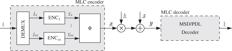
Figure 2.5 MLC: The encoder is formed by a demultiplexer,  parallel encoders, and a mapper. The decoder can be based on MSD or PDL
The decoding of MLC can be done using the principle of successive interference cancelation, known as multistage decoding (MSD). First, the first sequence ![]() is decoded using the channel outcome according to the ML principle (see (1.5)), i.e., by using the conditional PDF
is decoded using the channel outcome according to the ML principle (see (1.5)), i.e., by using the conditional PDF ![]() . Next, the decoding results
. Next, the decoding results ![]() (or equivalently
(or equivalently ![]() ) are passed to the second decoder. Assuming error-free decoding, i.e.,
) are passed to the second decoder. Assuming error-free decoding, i.e., ![]() , the second decoder can decode its own transmitted codeword using
, the second decoder can decode its own transmitted codeword using ![]() . As shown in Fig. 2.6 (a), this continues to the last stage where all the bits (except the last one) are known.
. As shown in Fig. 2.6 (a), this continues to the last stage where all the bits (except the last one) are known.

Figure 2.6 Decoding for MLC: (a) multistage decoding and (b) parallel decoding of the individual levels
Removing the interaction between the decoders and thus ignoring the relationships between the transmitted bitstreams ![]() results in what is known as parallel decoding of the individual levels (PDL), also shown in Fig. 2.6 (b). Then, the decoders operate in parallel, yielding a shorter decoding time at the price of decoding suboptimality.
results in what is known as parallel decoding of the individual levels (PDL), also shown in Fig. 2.6 (b). Then, the decoders operate in parallel, yielding a shorter decoding time at the price of decoding suboptimality.
In MLC, the selection of the ![]() rates of the codes is crucial. One way of doing this is based on information-theoretic arguments (which we will clarify in Section 4.4). One of the main issues when designing MLC is to take into account the decoding errors which propagate throughout the decoding process.
rates of the codes is crucial. One way of doing this is based on information-theoretic arguments (which we will clarify in Section 4.4). One of the main issues when designing MLC is to take into account the decoding errors which propagate throughout the decoding process.
2.3.3 Bit-Interleaved Coded Modulation
BICM was introduced in 1992 by Zehavi and later analyzed from an information-theoretic point of view by Caire et al. A general BICM system model is shown in Fig. 2.7 where the CM encoder in Fig. 2.3 is realized as a serial concatenation of a binary encoder (ENC) of rate ![]() , a bit-level interleaver
, a bit-level interleaver ![]() , and a mapper
, and a mapper ![]() .
.
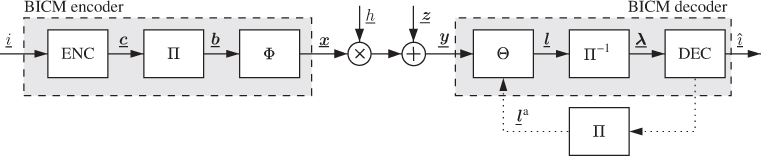
Figure 2.7 The BICM encoder is formed by a serial concatenation of a binary encoder (ENC), a bit-level interleaver ( ), and a memoryless mapper (
 ). The BICM decoder is composed of a demapper (
 ) that calculates the L-values, a deinterleaver, and a binary decoder (DEC). For a BICM with iterative demapping (BICM-ID) decoder, the channel decoder and the demapper exchange information in an iterative fashion
In the model in Fig. 2.7, any binary encoder can be used. The encoders we consider in this book are briefly introduced in Section 2.6. The interleaver ![]() permutes the codewords
permutes the codewords ![]() into the codewords
into the codewords ![]() . Thus, the interleaver may be seen as a one-to-one mapping between the channel code
. Thus, the interleaver may be seen as a one-to-one mapping between the channel code ![]() (i.e., all possible sequences
(i.e., all possible sequences ![]() ) and the code
) and the code ![]() . The interleaving is often modeled as a random permutation of the elements of the sequence
. The interleaving is often modeled as a random permutation of the elements of the sequence ![]() but of course, in practice, the permutation rules are predefined and known by both the transmitter and the receiver. More details about the interleaver are given in Section 2.7. The mapper
but of course, in practice, the permutation rules are predefined and known by both the transmitter and the receiver. More details about the interleaver are given in Section 2.7. The mapper ![]() operates the same way as before, i.e., there is a one-to-one mapping between length-
operates the same way as before, i.e., there is a one-to-one mapping between length-![]() binary vectors and constellation points.
binary vectors and constellation points.
The BICM decoder is composed of three mandatory elements: the demapper ![]() , the deinterleaver
, the deinterleaver ![]() , and the binary decoder DEC. The demapper
, and the binary decoder DEC. The demapper ![]() calculates the logarithmic-likelihood ratios (LLRs, or L-values) for each code bit in
calculates the logarithmic-likelihood ratios (LLRs, or L-values) for each code bit in ![]() . These L-values are then deinterleaved by
. These L-values are then deinterleaved by ![]() and the resulting permuted sequence of L-values
and the resulting permuted sequence of L-values ![]() is passed to the channel decoder DEC. The L-values are the basic signals exchanged in a BICM receiver. We analyze their properties in Chapters 3 and 5.
is passed to the channel decoder DEC. The L-values are the basic signals exchanged in a BICM receiver. We analyze their properties in Chapters 3 and 5.
Recognizing the BICM encoder as a concatenation of a binary encoder and an ![]() -ary mapper, the decoding can be done in an iterative manner. This is known as bit-interleaved coded modulation with iterative decoding/demapping (BICM-ID). In BICM-ID, the decoder and the demapper exchange information about the code bits using the so-called extrinsic L-values calculated alternatively by the demapper and the decoder. Soon after BICM-ID was introduced, binary labeling was recognized to play an important role in the design of BICM-ID transceivers and has been extensively studied in the literature.
-ary mapper, the decoding can be done in an iterative manner. This is known as bit-interleaved coded modulation with iterative decoding/demapping (BICM-ID). In BICM-ID, the decoder and the demapper exchange information about the code bits using the so-called extrinsic L-values calculated alternatively by the demapper and the decoder. Soon after BICM-ID was introduced, binary labeling was recognized to play an important role in the design of BICM-ID transceivers and has been extensively studied in the literature.
2.4 Channel Models
Although in practice the codebook is obtained in a deterministic way, we model ![]() as
as ![]() -dimensional independent random variables with PMF
-dimensional independent random variables with PMF ![]() (more details are given in Section 2.5.3), which is compatible with the assumption of the codebook
(more details are given in Section 2.5.3), which is compatible with the assumption of the codebook ![]() being randomly generated. Under these assumptions, and omitting the discrete-time index
being randomly generated. Under these assumptions, and omitting the discrete-time index ![]() , (2.24) can be modeled using random vectors
, (2.24) can be modeled using random vectors
where ![]() is an
is an ![]() -dimensional vector with independent and identically distributed (i.i.d.) Gaussian-distributed entries, so
-dimensional vector with independent and identically distributed (i.i.d.) Gaussian-distributed entries, so ![]() , where
, where ![]() is the power spectral density of the noise in (2.23).
is the power spectral density of the noise in (2.23).
The PDF of the channel output in (2.27), conditioned on the channel state ![]() and the transmitted symbol
and the transmitted symbol ![]() , is given by
, is given by
The channel gain ![]() models variations in the propagation medium because of phenomena such as signal absorption and fading2 and is captured by the PDF
models variations in the propagation medium because of phenomena such as signal absorption and fading2 and is captured by the PDF ![]() . Throughout this book, we assume that the receiver knows the channel realization perfectly, obtained using channel estimation techniques we do not cover.
. Throughout this book, we assume that the receiver knows the channel realization perfectly, obtained using channel estimation techniques we do not cover.
If we use the so-called fast-fading channel model, the channel gain ![]() is a random variable, so the instantaneous SNR in (2.29) is a random variable as well, i.e.,
is a random variable, so the instantaneous SNR in (2.29) is a random variable as well, i.e.,
As the average SNR depends on the parameters of three random variables, it is customary to fix two of them and vary the third. For the numerical results presented in this book, we keep constant the transmitted signal energy and the variance of the channel gain, i.e., ![]() and
and ![]() .
.
Each transmitted symbol conveys ![]() information bits, and thus, the relation between the average symbol energy
information bits, and thus, the relation between the average symbol energy ![]() and the average information bit energy
and the average information bit energy ![]() is given by
is given by ![]() . The average SNR can then be expressed as
. The average SNR can then be expressed as
2.5 The Mapper
An important element of the BICM transmitter in Fig. 2.7 is the mapper ![]() , which we show in Fig. 2.8. This mapper, using
, which we show in Fig. 2.8. This mapper, using ![]() bits as input, selects one of the symbols from the constellation to be transmitted. The mapper is then fully defined by the constellation
bits as input, selects one of the symbols from the constellation to be transmitted. The mapper is then fully defined by the constellation ![]() used for transmission and the way the bits are mapped to the constellation symbols. Although in a general case we can use many-to-one mappings (i.e.,
used for transmission and the way the bits are mapped to the constellation symbols. Although in a general case we can use many-to-one mappings (i.e., ![]() ), our analysis will be restricted to bijective mapping operations
), our analysis will be restricted to bijective mapping operations ![]() , i.e., when
, i.e., when ![]() .
.
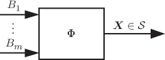
Figure 2.8 The role of the mapper  in Fig. 2.7 is to generate the symbols from the constellation
  using
using  binary inputs
2.5.1 Constellation
The constellation used for transmission is denoted by ![]() , and the constellation symbols by
, and the constellation symbols by ![]() , where
, where ![]() . The difference between two constellation symbols is defined as
. The difference between two constellation symbols is defined as
The constellation Euclidean distance spectrum (CEDS) is defined via a vector ![]() . The CEDS contains all the
. The CEDS contains all the ![]() possible distances between pairs of constellation points in
possible distances between pairs of constellation points in ![]() , where
, where ![]() . The minimum Euclidean distance (MED) of the constellation is defined as the smallest element of the CEDS, i.e.,
. The minimum Euclidean distance (MED) of the constellation is defined as the smallest element of the CEDS, i.e.,
where from now on we use ![]() to enumerate all the constellation points in
to enumerate all the constellation points in ![]() .
.
The input distribution is defined by the vector
For a uniform distribution, i.e., where all the symbols are equiprobable, we use the notation
We assume that the constellation ![]() is defined so that the transmitted symbols
is defined so that the transmitted symbols ![]() have zero mean
have zero mean
and, according to the convention we have adopted, the average symbol energy ![]() is normalized as
is normalized as
We will often refer to the practically important constellations pulse amplitude modulation (PAM), phase shift keying (PSK), and quadrature amplitude modulation (QAM), defined as follows:
- An
 PSK constellation is defined as
2.45
PSK constellation is defined as
2.45
where
 . In Fig. 2.9, three commonly used
  PSK constellations are shown. For 8PSK, we also show the vector
  in (2.39) as well as the MED (2.40). For
  , (2.43) and (2.44) are satisfied.
 - An
 PAM constellation is defined as
2.46
PAM constellation is defined as
2.46
where the CEDS is
 with
with  . For
. For  ,2.47
,2.47
- A rectangular
 QAM constellation is defined as the Cartesian product of two
  PAM constellations, i.e.,
2.48
PAM constellations, i.e.,
2.48
where
 ,
,  , and
, and  .
. - A square
 QAM is obtained as a particular case of a rectangular
  QAM when
  . In this case, we have
  . Again, for a uniform input distribution
  , to guarantee (2.43) and (2.44), we will use the scaling
2.49
, to guarantee (2.43) and (2.44), we will use the scaling
2.49
The MED is
 .
.

Figure 2.9  PSK constellations
  for (a)
  , (b)
, (b)  , and (c)
  . The vector
  in (2.39) and the MED in (2.40) for 8PSK are shown
One of the simplest constellations we will refer to is 2PAM, which is equivalent to 2PSK and is also known as binary phase shift keying (BPSK). Constellations with more than two constellation points are discussed in the following example.

Figure 2.10  PAM constellations
  for (a)
  , (b)
, (b)  , and (c)
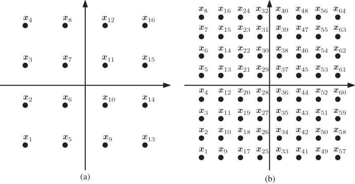
Figure 2.11 Square  QAM constellations
  for (a)
  and (b)
  . The 16QAM constellation is generated as the Cartesian product of two 4PAM constellations (shown in Fig. 2.10 (b)) and the 64QAM as the Cartesian product of two 8PAM constellations (shown in Fig. 2.10 (c))
Up to this point, we have considered the input constellation to be a set ![]() . As we will later see, it is useful to represent the constellation symbols taken from the constellation
. As we will later see, it is useful to represent the constellation symbols taken from the constellation ![]() in an ordered manner via the
in an ordered manner via the ![]() matrix
matrix ![]() . Using this definition, the elements of
. Using this definition, the elements of ![]() are
are ![]() with
with ![]() , and the elements of
, and the elements of ![]() are
are ![]() with
with ![]() . This notation will be useful in Section 2.5.2 where binary labelings are defined.
. This notation will be useful in Section 2.5.2 where binary labelings are defined.
Another reason for using the notation ![]() for a constellation is that with such a representation, 2D constellations generated via Cartesian products (such as rectangular
for a constellation is that with such a representation, 2D constellations generated via Cartesian products (such as rectangular ![]() QAM constellations) can also be defined using the ordered direct product defined in (2.2). A rectangular
QAM constellations) can also be defined using the ordered direct product defined in (2.2). A rectangular ![]() QAM constellation is then defined by the matrix
QAM constellation is then defined by the matrix ![]() formed by the ordered direct product of two
formed by the ordered direct product of two ![]() PAM constellations
PAM constellations ![]() and
and ![]() , i.e.,
, i.e.,
The notation used in (2.55) (or more generally in (2.53)) will be used in Section 2.5.2 to formally define the binary labeling of 2D constellations.
We note that although the 4PSK constellation in Fig. 2.9 (a) is equivalent to 4QAM (generated as ![]() ), the ordering used in Fig. 2.9 (a) is different, i.e., we use a more natural ordering for
), the ordering used in Fig. 2.9 (a) is different, i.e., we use a more natural ordering for ![]() PSK constellations, namely, a counterclockwise enumeration of the constellation points.
PSK constellations, namely, a counterclockwise enumeration of the constellation points.
2.5.2 Binary Labeling
The mapper ![]() is defined as a one-to-one mapping of a length-
is defined as a one-to-one mapping of a length-![]() binary codeword to a constellation symbol, i.e.,
binary codeword to a constellation symbol, i.e., ![]() . To analyze the mapping rule of assigning all length-
. To analyze the mapping rule of assigning all length-![]() binary labels to the symbols
binary labels to the symbols ![]() , we define the binary labeling of the
, we define the binary labeling of the ![]() constellation
constellation ![]() as an
as an ![]() binary matrix
binary matrix ![]() , where
, where ![]() is the binary label of the constellation symbol
is the binary label of the constellation symbol ![]() .
.
The labeling universe is defined as a set ![]() of binary matrices
of binary matrices ![]() with
with ![]() distinct columns. All the different binary labelings can be obtained by studying all possible column permutations of a given matrix
distinct columns. All the different binary labelings can be obtained by studying all possible column permutations of a given matrix ![]() , and thus, there are
, and thus, there are ![]() different ways to label a given
different ways to label a given ![]() -ary constellation.3 Some of these labelings have useful properties. In the following, we define those which are of particular interest.
-ary constellation.3 Some of these labelings have useful properties. In the following, we define those which are of particular interest.
According to Definition 2.8, a constellation is Gray-labeled if all pairs of constellation points at MED have labels that differ only in one bit. As this definition depends on the constellation ![]() , a labeling construction is not always available; in fact, the existence of a Gray labeling cannot be guaranteed in general. However, it can be obtained for the constellations
, a labeling construction is not always available; in fact, the existence of a Gray labeling cannot be guaranteed in general. However, it can be obtained for the constellations ![]() and
and ![]() we focus on.
we focus on.
While Gray labelings are not unique (for a given constellation ![]() , in general, there is more than one
, in general, there is more than one ![]() satisfying Definition 2.8), the most popular one is the binary reflected Gray code (BRGC), whose construction is given below. Throughout this book, unless stated otherwise, we use the BRGC, normally referred to in the literature as “Gray labeling”, “Gray coding”,4 or “Gray mapping”.
satisfying Definition 2.8), the most popular one is the binary reflected Gray code (BRGC), whose construction is given below. Throughout this book, unless stated otherwise, we use the BRGC, normally referred to in the literature as “Gray labeling”, “Gray coding”,4 or “Gray mapping”.
In Fig. 2.12, we show how the BRGC of order ![]() is recursively constructed.
is recursively constructed.

Figure 2.12 Recursive expansions of the labeling  used to generate the BRGC of order
The importance of the BRGC is due to the fact that for all the constellations defined in Section 2.5, the BRGC (i) minimizes the bit-error probability (BEP) when the SNR tends to infinity and (ii) gives high achievable rates in BICM transmission for medium to high SNR. More details about this are given in Chapter 4.
Another labeling of particular interest is the natural binary code (NBC). The NBC is relevant for BICM because it maximizes its achievable rates for ![]() PAM and
PAM and ![]() QAM constellations in the low SNR regime. For
QAM constellations in the low SNR regime. For ![]() PAM and
PAM and ![]() QAM constellations, the NBC is also one of the most natural ways of implementing Ungerboeck's SP labeling, and thus, it is very often used in the design of TCM systems.
QAM constellations, the NBC is also one of the most natural ways of implementing Ungerboeck's SP labeling, and thus, it is very often used in the design of TCM systems.
If we denote the entries of ![]() and
and ![]() by
by ![]() and
and ![]() for
for ![]() and
and ![]() , we find that
, we find that ![]() and
and ![]() for
for ![]() . Alternatively, we have
. Alternatively, we have ![]() for
for ![]() , or, in matrix notation,
, or, in matrix notation, ![]() and
and ![]() , where
, where
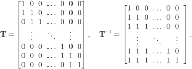
In (2.59), we highlighted in bold each first nonzero element of the ![]() th row of the labeling matrix. These elements are called the pivots of
th row of the labeling matrix. These elements are called the pivots of ![]() , and are used in the following definition.
, and are used in the following definition.
The matrix ![]() for
for ![]() in Example 2.13 (or more generally
in Example 2.13 (or more generally ![]() for any
for any ![]() ) is a reduced column echelon matrix while
) is a reduced column echelon matrix while ![]() is not because it does not fulfill the first condition in Definition 2.14.
is not because it does not fulfill the first condition in Definition 2.14.
Other binary labelings of interest include the folded binary code (FBC) and the binary semi-Gray code (BSGC). These labelings, together with that for the BRGC are shown in Fig. 2.13 for an 8PAM constellation.

Figure 2.13 8PAM labeled constellations: (a) BRGC, (b) NBC, (c) FBC, and (d) BSGC
Square and rectangular ![]() QAM constellations are relevant in practice, and also very popular for BICM systems. In what follows, we describe one of the most common ways of labeling an
QAM constellations are relevant in practice, and also very popular for BICM systems. In what follows, we describe one of the most common ways of labeling an ![]() QAM constellation using the BRGC. Although we show it for the BRGC, the following way of labeling QAM constellations can also be used with the NBC, FBC, or BSGC. It is also important to notice at this point that to unequivocally define the labeling of a 2D constellation, the use of the ordered constellation points (via
QAM constellation using the BRGC. Although we show it for the BRGC, the following way of labeling QAM constellations can also be used with the NBC, FBC, or BSGC. It is also important to notice at this point that to unequivocally define the labeling of a 2D constellation, the use of the ordered constellation points (via ![]() ) is needed.
) is needed.
Again, a square ![]() QAM is a particular case of Definition 2.15 when
QAM is a particular case of Definition 2.15 when ![]() . One particularly appealing property of this labeling is that the first and second dimension of the constellation are decoupled in terms of the binary labeling. This is important because it reduces the complexity of the L-values' computation by the demapper.
. One particularly appealing property of this labeling is that the first and second dimension of the constellation are decoupled in terms of the binary labeling. This is important because it reduces the complexity of the L-values' computation by the demapper.

Figure 2.14 Constellations labeled by the BRGC: (a) 4QAM and (b) 16QAM
It is important to note that ![]() in (2.61) and (2.62) do not coincide with the definition of the BRGC in Definition 2.10. This is because each constituent labeling is a BRGC; however, the ordered direct product of two BRGC labelings is not necessarily a BRGC.
in (2.61) and (2.62) do not coincide with the definition of the BRGC in Definition 2.10. This is because each constituent labeling is a BRGC; however, the ordered direct product of two BRGC labelings is not necessarily a BRGC.

Figure 2.15 16QAM constellation with the M16 labeling
For our considerations, it is convenient to define the subconstellations
We also define ![]() where
where ![]() as the set of indices to all the symbols in
as the set of indices to all the symbols in ![]() , i.e.,
, i.e., ![]() .
.
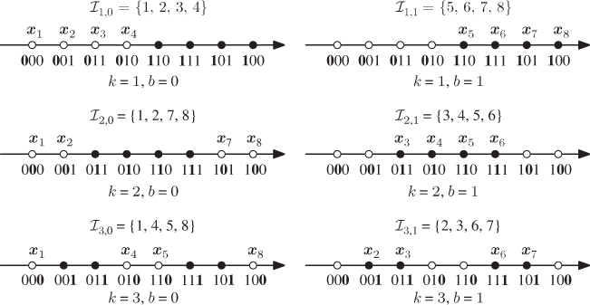
Figure 2.16 Subconstellations  for 8PAM labeled by the BRGC from Fig. 2.13 (a), where the values of
  for
for  are highlighted. The values of
  are also shown
We conclude this section by discussing the labeling by SP, initially proposed by Ungerboeck for TCM. To formally define this idea for a given constellation ![]() and labeling
and labeling ![]() , we define the subsets
, we define the subsets ![]() for
for ![]() , where
, where
Additionally, we define the minimum intra-ED at level ![]() as
as
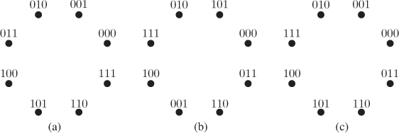
Figure 2.17 Three SP labelings: (a) NBC, (b) SSP, and (c) MSP
2.5.3 Distribution and Shaping
Signal shaping refers to the use of nonequally spaced and/or nonequiprobable constellation symbols. The need for shaping may be understood using an information-theoretic argument: the mutual information (MI) ![]() can be increased by optimizing the distribution
can be increased by optimizing the distribution ![]() in (2.41) for a given constellation
in (2.41) for a given constellation ![]() (probabilistic shaping), by changing the constellation
(probabilistic shaping), by changing the constellation ![]() for a given
for a given ![]() (geometrical shaping) or by optimizing both (mixed shaping). This argument relates to the random-coding principle, so it may be valid when capacity-approaching codes are used. In other cases (e.g., when convolutional codes (CCs) are used), different shaping principles might be devised because the MI is not necessarily a good indicator for the actual performance of the decoder.
(geometrical shaping) or by optimizing both (mixed shaping). This argument relates to the random-coding principle, so it may be valid when capacity-approaching codes are used. In other cases (e.g., when convolutional codes (CCs) are used), different shaping principles might be devised because the MI is not necessarily a good indicator for the actual performance of the decoder.
We will assume that ![]() are independent binary random variables. Sufficient conditions for this independence in the case of CENCs are given in Section 2.6.2. Moreover, even if in most cases the bits are i.u.d., nonuniform bit distributions can be imposed by an explicit injection of additional ones or zeros. This allows us to obtain
are independent binary random variables. Sufficient conditions for this independence in the case of CENCs are given in Section 2.6.2. Moreover, even if in most cases the bits are i.u.d., nonuniform bit distributions can be imposed by an explicit injection of additional ones or zeros. This allows us to obtain ![]() , and thus, the entire distribution is characterized by the vector
, and thus, the entire distribution is characterized by the vector
The probability of the transmitted symbols is given by
or equivalently, by
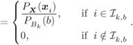
For future use, we define the conditional input symbol probabilities as

When the bits are uniformly distributed (u.d.) (i.e., ![]() ), we obtain a uniform input symbol distributions, i.e.,
), we obtain a uniform input symbol distributions, i.e.,
and