
Chapter 6
Performance Evaluation
This chapter describes different methods that can be used to evaluate the performance of bit-interleaved coded modulation (BICM) receivers. We focus on bit-error probability (BEP), symbol-error probability (SEP), and word-error probability (WEP) as performance metrics, as these are often considered relevant in practical systems. We pay special attention to techniques based on the knowledge of the probability density function (PDF) of the L-values we developed in Chapter 5, and in particular to the Gaussian models introduced in Section 5.5.
This chapter is organized as follows. In Section 6.1 we review methods to evaluate the performance for uncoded transmission and in Section 6.2 we study the performance of decoders (i.e., coded transmission). Section 6.3 is devoted to analyzing the pairwise-error probability (PEP), which appears as the key quantity when evaluating coded transmission. Section 6.4 studies the performance of BICM based on the Gaussian approximations of the PDF of the L-values.
6.1 Uncoded Transmission
By uncoded transmission we mean that the channel coding is absent (or is ignored), and thus, the decision on the transmitted symbols is made without taking into account the sequence of symbols (i.e., the constraints on the codewords). We are instead interested in deciding which symbol was transmitted at a given time instant ![]() using the channel output
using the channel output ![]() . These are “hard decisions” (briefly discussed in Section 3.4) which might eventually be fed to the channel decoder.
. These are “hard decisions” (briefly discussed in Section 3.4) which might eventually be fed to the channel decoder.
The criterion for making a hard decision depends on how it will be used. Probably the simplest and most intuitive approach is to minimize the SEP. Assuming an additive white Gaussian noise (AWGN) channel and equally likely symbols, we then obtain the expression we already showed in (3.100), i.e.,

Similarly, assuming equally likely bits, to minimize the BEP, the decision on the transmitted bits is
which can also be expressed as

or in terms of L-values, as

From (6.4) we conclude that a hard decision on the transmitted bits is equivalent to making a decision on the sign of the L-values in (3.50).1
The implementation of (6.3) has a complexity dominated by the calculation of the sum of exponential functions so simplifications may be sought. In particular, we may apply the max-log approximation, which used in (6.3) gives
The hard decision on the bits shown in (6.5) is also equivalent to determining the sign of the L-values calculated via the max-log approximation (i.e., when ![]() in (6.4) are max-log L-values). This was already shown in (3.106).
in (6.4) are max-log L-values). This was already shown in (3.106).
As we showed in Theorem 3.17, the decision in (6.5) is equivalent to the decision in (6.1), and thus, we can consider the vector of hard decisions on the bits
where ![]() . Owing to this equivalence we focus on the symbol-wise hard decisions in (6.1), or equivalently, on the bitwise hard decisions in (6.6) based on max-log L-values.
. Owing to this equivalence we focus on the symbol-wise hard decisions in (6.1), or equivalently, on the bitwise hard decisions in (6.6) based on max-log L-values.
Since the hard decisions are equivalent to a one-bit (sign only) quantization of the L-values, we may continue to view them as a part of the BICM channel, which now becomes a binary-input binary-output channel. Methods for analyzing the performance of such a BICM channel in terms of SEP or BEP for uncoded transmission have been studied in the communication theory community over decades. The main reason for focusing on these quantities is that SEP/BEP for uncoded transmission are relatively easy to obtain compared to similar quantities in coded transmission. The underlying assumption is that systems with the same SEP/BEP will perform similarly when coding/decoding is added. As we will see in Chapter 8, this is, in general not true, as the design of the interleaver may change the performance of the coded transmission, while uncoded transmission is unaffected by interleaving.
6.1.1 Decision Regions
The SEP is defined as
where
where the decision region of the symbol ![]() is defined using (6.1) as
is defined using (6.1) as
and where ![]() is given by (3.54).
is given by (3.54).
The set ![]() is the so-called Voronoi region of the symbol
is the so-called Voronoi region of the symbol ![]() . In many practically relevant cases, the form of the Voronoi regions can be found by inspection. For example, when the constellation points are located on a rectangular grid (i.e., for
. In many practically relevant cases, the form of the Voronoi regions can be found by inspection. For example, when the constellation points are located on a rectangular grid (i.e., for ![]() -ary quadrature amplitude modulation (
-ary quadrature amplitude modulation (![]() QAM) constellations) or on a circle (i.e., for
QAM) constellations) or on a circle (i.e., for ![]() -ary phase shift keying (
-ary phase shift keying (![]() PSK) constellations), finding the decision regions
PSK) constellations), finding the decision regions ![]() consists in determining the closest constellation points to the symbol
consists in determining the closest constellation points to the symbol ![]() along each dimension of the grid. In the case of
along each dimension of the grid. In the case of ![]() QAM there are at most four such symbols, and in the case of
QAM there are at most four such symbols, and in the case of ![]() PSK constellations there are only two of them. In the more general case of irregular constellations, the Voronoi regions may be found using numerical routines.
PSK constellations there are only two of them. In the more general case of irregular constellations, the Voronoi regions may be found using numerical routines.
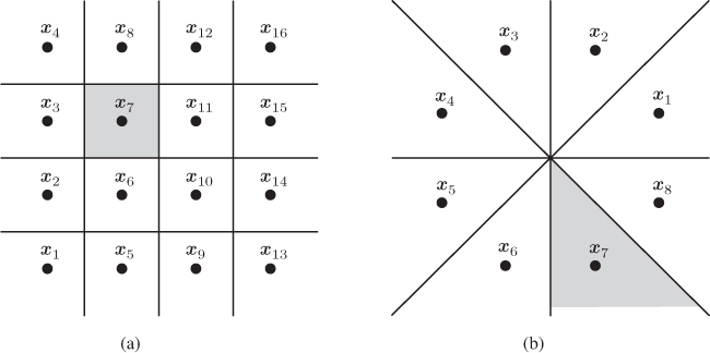
Figure 6.1 Voronoi regions for (a) 16QAM and (b) 8PSK constellations. The Voronoi region  is highlighted with gray
Let ![]() be the probability of detecting
be the probability of detecting ![]() when
when ![]() was transmitted, i.e.,
was transmitted, i.e.,
From now on, we refer to ![]() as the transition probability (TP).
as the transition probability (TP).
Using (6.12), the SEP (6.8) can then be expressed as
where to pass from (6.15) to (6.16) we used (6.9).
The BEP for the ![]() th bit was already defined in (3.110) for max-log metrics.2 For exact L-values, we have the following analogous definition
th bit was already defined in (3.110) for max-log metrics.2 For exact L-values, we have the following analogous definition
where ![]() are given by (6.3) and (6.4) and the “decision regions” for the
are given by (6.3) and (6.4) and the “decision regions” for the ![]() th bit are thus
th bit are thus

Similarly, in the case of max-log L-values, for the ![]() th bit in (3.110) with
th bit in (3.110) with ![]() given by (6.5), the BEP is expressed as
given by (6.5), the BEP is expressed as
where the decision regions in this case are
which follows from the fact that ![]() is the
is the ![]() th bit of the label of the detected symbol via (6.1) (see (6.6)).
th bit of the label of the detected symbol via (6.1) (see (6.6)).

Figure 6.2 Decision regions  (light gray) and
  (dark gray) in (6.20) for 16QAM with the M16 labeling shown in Fig. 2.5: (a)
  ,
,  ; (b)
; (b)  ,
,  ; (c)
; (c)  ,
,  ; and (d)
  ,
,  . The subconstellations
  and
and  are indicated, respectively, with white and black circles
The calculation of ![]() in (6.18) requires integration over the decision region
in (6.18) requires integration over the decision region ![]() , i.e.,
, i.e.,
This is in general quite difficult, mainly because ![]() is defined via nonlinear equations in (6.20) which, moreover, depend on
is defined via nonlinear equations in (6.20) which, moreover, depend on ![]() (as we showed in Example 6.2).
(as we showed in Example 6.2).
On the other hand, with the max-log approximation, the decision region ![]() is the union of the Voronoi regions
is the union of the Voronoi regions ![]() in (6.10), and thus, (i) it is independent of the SNR and (ii) it is defined via linear equations only. The BEP in this case is calculated as
in (6.10), and thus, (i) it is independent of the SNR and (ii) it is defined via linear equations only. The BEP in this case is calculated as
where (6.24) follows from the law of total probability, (6.25) from (6.10) and (6.21), and where the ![]() is given by (6.12). The BEP averaged over the bits' positions is then defined as
is given by (6.12). The BEP averaged over the bits' positions is then defined as
where ![]() is the Hamming distance (HD) between the binary labels of
is the Hamming distance (HD) between the binary labels of ![]() and
and ![]() , and where to pass from (6.27) to (6.28) we simply reorganized the summations.
, and where to pass from (6.27) to (6.28) we simply reorganized the summations.
From (6.16) and (6.28) we see that once the Voronoi regions ![]() in (6.10) are found, the challenge of calculating the SEP and BEP is reduced to the calculation of the TPs
in (6.10) are found, the challenge of calculating the SEP and BEP is reduced to the calculation of the TPs ![]() in (6.12). The problem then boils down to efficiently calculating the integral (6.14). This is the focus of the following sections.
in (6.12). The problem then boils down to efficiently calculating the integral (6.14). This is the focus of the following sections.
6.1.2 Calculating the Transition Probability
Before proceeding further, we express the Voronoi regions in (6.11) using the ![]() nonredundant inequalities defining
nonredundant inequalities defining ![]() , i.e.,
, i.e.,
where the linear forms in this case are
We use an arbitrary variable ![]() to index the nonredundant inequalities defining the region, and thus, the definitions in (6.29) and (6.30) are similar to those we already used in (5.87) and (5.88).3
to index the nonredundant inequalities defining the region, and thus, the definitions in (6.29) and (6.30) are similar to those we already used in (5.87) and (5.88).3
We start by analyzing the simplest possible case where only one nonredundant inequality ![]() exists (i.e.,
exists (i.e., ![]() ). In this case, the problem is one-dimensional, and thus, the Voronoi region
). In this case, the problem is one-dimensional, and thus, the Voronoi region ![]() is a half-space. In this case, we express the TP in (6.14) as
is a half-space. In this case, we express the TP in (6.14) as
where with slight abuse of notation we use ![]() in
in ![]() (without the argument
(without the argument ![]() ) to denote the parameters
) to denote the parameters ![]() and
and ![]() defining the linear form
defining the linear form ![]() in (6.30). The TP in (6.31) can be expressed as
in (6.30). The TP in (6.31) can be expressed as
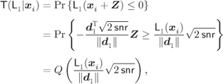
where (6.32) follows from the fact that ![]() is a zero-mean, unit variance Gaussian random variable.
is a zero-mean, unit variance Gaussian random variable.
The result shown in Example 6.3 can also be obtained by simple inspection: because the symbol ![]() is at distance
is at distance ![]() from the limit of the decision region
from the limit of the decision region ![]() , and the noise
, and the noise ![]() is Gaussian with variance
is Gaussian with variance ![]() , the calculation of
, the calculation of ![]() yields (6.33). Nevertheless, we use the formalism of the decision region defined by the line
yields (6.33). Nevertheless, we use the formalism of the decision region defined by the line ![]() for illustrative purposes.
for illustrative purposes.
The next step is to consider the region defined by two nonredundant inequalities ![]() and
and ![]() (i.e.,
(i.e., ![]() ). In this case, the Voronoi region
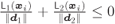
). In this case, the Voronoi region ![]() is a wedge, which we define in analogy to (5.95) as
is a wedge, which we define in analogy to (5.95) as
For convenience, we also define a “complementary” wedge
The wedges ![]() and
and ![]() are schematically shown in Fig. 6.3. These simple forms of
are schematically shown in Fig. 6.3. These simple forms of ![]() are important because they appear, e.g., in the case of
are important because they appear, e.g., in the case of ![]() PSK constellations (see Fig. 6.1). As we will see later, the analysis of a wedge also leads to expressions that can be used to study
PSK constellations (see Fig. 6.1). As we will see later, the analysis of a wedge also leads to expressions that can be used to study ![]() PAM,
PAM, ![]() QAM, as well as arbitrary constellations.
QAM, as well as arbitrary constellations.
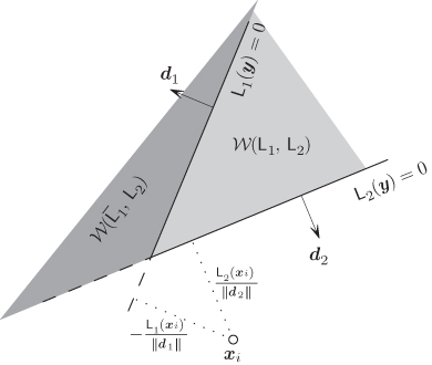
Figure 6.3 The wedges  and
and  are delimited by the lines
  and
and  . The distances from
  to the lines (the length of the dotted lines) are
  and
and 
For the case of the Voronoi region being a wedge, we denote the TP in (6.14) as
where in analogy to (5.96)
The TP in (6.37) can be expressed as
where
Owing to the normalization, ![]() and
and ![]() can be shown to be zero-mean, unit-variance Gaussian random variables with correlation
can be shown to be zero-mean, unit-variance Gaussian random variables with correlation
Using (6.41)–(6.44) (6.37) can be expressed as

where ![]() is given by (2.11).4
is given by (2.11).4
In the same way we defined a complementary wedge in (6.35), we define a “complementary” TP as
Following similar steps to those in (6.39)–(6.45), we find that the complementary TP in (6.46) is given by
The general expression (6.45) for the TP when the Voronoi region is a wedge particularizes to two interesting cases, which are shown schematically in Fig. 6.4.

Figure 6.4 In two particular cases, 2D integration can be obtained via 1D integrals. (a) When the lines  and
and  are orthogonal, the 2D integral is the product of two 1D integrals calculated independently along each of the orthogonal directions. (b) When the lines are parallel, the 2D integral becomes a difference of 1D integrals
- When
 , the lines
  and
and  are orthogonal, and thus, the variables
  ,
,  in (6.41) are independent. We then obtain
  , and thus,
- When
 , the lines
  and
and  are parallel, and thus, the wedge
  “degenerates” into a stripe. In this case, the variables in (6.41) satisfy
  , and thus, using
  in (2.12), we obtain
6.50
in (2.12), we obtain
6.50
which is valid for
 (see (2.12)), i.e., when the linear inequalities are not contradictory. The 2D integral is thus reduced to a 1D integration of a zero-mean Gaussian PDF along a line orthogonal to the stripe's limits.
With the expressions we have developed in (6.32) and (6.49), we are in a position to compute the SEP and BEP for any 1D constellation. In the following example we show how to do this for 4PAM and the binary reflected Gray code (BRGC).
As we showed in Example 6.4, the TP need not always be calculated for all pairs of the transmitted symbols. Instead, the regularity and the symmetry of the constellation can be exploited to simplify the calculations. This can also be done for 2D constellation as we show in the following example.

Figure 6.5 In  PSK constellations, the decision region
  is a wedge defined by the two symbols closest to
The expressions we derived in the previous example are entirely general; yet, particular cases of ![]() PSK constellations lead to simpler results that do not need bivariate Q-functions or, in fact, exploit the simplicity of the particular cases we analyzed in (6.48) and (6.49). We show this in the following example.
PSK constellations lead to simpler results that do not need bivariate Q-functions or, in fact, exploit the simplicity of the particular cases we analyzed in (6.48) and (6.49). We show this in the following example.

Figure 6.6 Decision regions  for an 8PSK constellation labeled by the BRGC: (a)
  and (b)
In Example 6.5 we were able to express ![]() for
for ![]() PSK constellation using bivariate Q-functions. Our objective now is to do the same in the case of an arbitrary 2D constellation. First, we assume that
PSK constellation using bivariate Q-functions. Our objective now is to do the same in the case of an arbitrary 2D constellation. First, we assume that ![]() is a closed polygon defined by
is a closed polygon defined by ![]() linear forms
linear forms ![]() corresponding to the polygon's sides. We assume that the linear pieces are enumerated counter-clockwise, as shown in Fig. 6.7. In such a case, using the complementary wedge we defined in (6.35), the whole space can be expressed as a union of disjoint sets, i.e.,
corresponding to the polygon's sides. We assume that the linear pieces are enumerated counter-clockwise, as shown in Fig. 6.7. In such a case, using the complementary wedge we defined in (6.35), the whole space can be expressed as a union of disjoint sets, i.e.,
The TP in (6.12) can then be expressed as
where ![]() is given by (6.46).
is given by (6.46).

Figure 6.7 If the decision region  is a polygon delimited by the lines
  , the observation space can be represented as a union of
  and complementary wedges
Similarly, if ![]() is an “infinite” polygon as shown in Fig. 6.8, we can write
is an “infinite” polygon as shown in Fig. 6.8, we can write
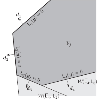
Figure 6.8 If the decision region is an infinite polygon, the TP can be expressed using a sum of integrals over wedges and complementary wedges
and then,
We conclude then that the TPs for any 2D constellation can be calculated using only functions ![]() , which as we showed before, are expressed in terms of bivariate Q-function. These bivariate Q-functions now play the same role that the Q-function has when calculating
, which as we showed before, are expressed in terms of bivariate Q-function. These bivariate Q-functions now play the same role that the Q-function has when calculating ![]() for 1D constellations.
for 1D constellations.