
Chapter 5
Probability Density Functions of L-values
To characterize complex systems such as bit-interleaved coded modulation (BICM) receivers, it is convenient to study their building blocks independently. An important building block in a BICM receiver is the demapper ![]() , whose role consists in calculating the L-values. In this chapter, we formally describe its behavior from a probabilistic point of view. The models developed here will be used in the chapters that follow, to study the performance of BICM transceivers.
, whose role consists in calculating the L-values. In this chapter, we formally describe its behavior from a probabilistic point of view. The models developed here will be used in the chapters that follow, to study the performance of BICM transceivers.
This chapter is organized as follows. Section 5.1 motivates the need for finding the probability density function (PDF) of the L-values and shows its challenges. Sections 5.2 and 5.3 explain how to calculate the PDFs for 1D and 2D constellations, respectively. PDFs of the L-values in fading channels are discussed in Section 5.4 and Gaussian approximations are provided in Section 5.5.
5.1 Introduction and Motivation
5.1.1 BICM Channel
The BICM channel is defined as the entity that encompasses the interleaver, the mapper, the channel, the demapper, and the deinterleaver, as shown in Fig. 5.1. As the off-the-shelf binary encoder/decoder used in BICM operates “blindly” with respect to the channel, the BICM channel corresponds to an equivalent binary-input continuous-output (BICO) channel that separates the binary encoder and decoder.

Figure 5.1 The BICM channel provides a single interface, which models the effect of the interleaver, the mapper  , the channel, the demapper
  , and the deinterleaver
At the output of the BICM channel, we obtain a sequence of L-values ![]() . However, because the interleaving is a one-to-one operation, without loss of generality, we can focus on the sequence of L-values at the output of the demapper
. However, because the interleaving is a one-to-one operation, without loss of generality, we can focus on the sequence of L-values at the output of the demapper ![]() instead. This observation can lead us to define a different BICM channel as shown in Fig. 5.2. In this new model, the interleaver and the deinterleaver become parts of the binary encoder and the decoder, respectively, showing that setting boundaries of the “BICM channel” interface is somewhat arbitrary. Regardless of whether we use the model in Fig. 5.1 or the one in Fig. 5.2, we recognize the demapper
instead. This observation can lead us to define a different BICM channel as shown in Fig. 5.2. In this new model, the interleaver and the deinterleaver become parts of the binary encoder and the decoder, respectively, showing that setting boundaries of the “BICM channel” interface is somewhat arbitrary. Regardless of whether we use the model in Fig. 5.1 or the one in Fig. 5.2, we recognize the demapper ![]() as the key component in the receiver.
as the key component in the receiver.
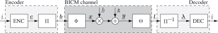
Figure 5.2 The BICM channel here provides the single interface that models the effect of the mapper  , the channel, and the demapper
  . The interleaver and the deinterleaver become parts of the binary encoder and the decoder, respectively
The model from Fig. 5.2 indicates that the L-values ![]() in (3.50) are functions of the channel outcome
in (3.50) are functions of the channel outcome ![]() , which is a random variable. The L-values are then functions of a random variable, and thus, are also random variables. Therefore, from now on, we use
, which is a random variable. The L-values are then functions of a random variable, and thus, are also random variables. Therefore, from now on, we use ![]() to denote the L-values. To obtain the PDF of
to denote the L-values. To obtain the PDF of ![]() conditioned on the bit
conditioned on the bit ![]() , we marginalize its PDF over all the symbols in
, we marginalize its PDF over all the symbols in ![]() , i.e.,
, i.e.,
To pass from (5.1) to (5.2) we used (2.77) and to pass from (5.2) to (5.3) we use the fact that for any ![]() , conditioning on the symbol and the
, conditioning on the symbol and the ![]() th bit is equivalent to conditioning on the symbol only.
th bit is equivalent to conditioning on the symbol only.
From the model in Fig. 5.1, we see that the outputs of the BICO channel are the deinterleaved L-values ![]() , which are next passed to the decoder. These L-values are also random variables, which we denote by
, which are next passed to the decoder. These L-values are also random variables, which we denote by ![]() . Under some assumptions on the interleaver structure, it can be shown that the L-values passed to the decoder are independent and identically distributed (i.i.d.) random variables with PDF1
. Under some assumptions on the interleaver structure, it can be shown that the L-values passed to the decoder are independent and identically distributed (i.i.d.) random variables with PDF1
where ![]() is a binary random variable that models the input to the BICM channel in Fig. 5.1.
is a binary random variable that models the input to the BICM channel in Fig. 5.1.
The rest of this chapter is aimed at characterizing the PDFs ![]() , which owing to (5.3) and (5.4), allows us to model the BICM channels in Figs. 5.1 and 5.2. The explicit objective of the modeling is to develop analytical tools for performance evaluation, e.g., in terms of bit-error probability (BEP). This is necessary because, even if the performance may be evaluated via Monte Carlo integration, analytical forms simplify the calculations and provide insight into relevant design parameters.
, which owing to (5.3) and (5.4), allows us to model the BICM channels in Figs. 5.1 and 5.2. The explicit objective of the modeling is to develop analytical tools for performance evaluation, e.g., in terms of bit-error probability (BEP). This is necessary because, even if the performance may be evaluated via Monte Carlo integration, analytical forms simplify the calculations and provide insight into relevant design parameters.
5.1.2 Case Study: PDF of L-values for 4PAM
While it is simple to obtain the PDF of the L-values in the case of a 2PAM constellation (see Section 3.3.1), the case of an ![]() -ary constellation is more challenging. In this section, we show an example to illustrate the difficulty of tackling this problem without any simplification.
-ary constellation is more challenging. In this section, we show an example to illustrate the difficulty of tackling this problem without any simplification.
We consider the additive white Gaussian noise (AWGN) channel and the simplest case of a multilevel 1D constellation (![]() ), i.e., a constellation with
), i.e., a constellation with ![]() points, which is well exemplified by a 4PAM constellation defined in Section 2.5. The labeling used is the binary reflected Gray code (BRGC),2 i.e.,
points, which is well exemplified by a 4PAM constellation defined in Section 2.5. The labeling used is the binary reflected Gray code (BRGC),2 i.e.,
The constellation and labeling are shown in Fig. 5.3.
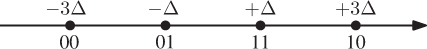
Figure 5.3 4PAM constellation labeled by the BRGC
Throughout this chapter, we use ![]() introduced in Section 3.3.1 to denote the functional relationship between
introduced in Section 3.3.1 to denote the functional relationship between ![]() and
and ![]() . We start by calculating the PDF of the L-value
. We start by calculating the PDF of the L-value ![]() for the bit position
for the bit position ![]() , for which the relation between
, for which the relation between ![]() and the observation
and the observation ![]() in (3.50) is given by3
in (3.50) is given by3

where
For the case of a 4PAM constellation, ![]() .
.
The relationship (5.6) is shown in Fig. 5.4 for different values of ![]() , where the nonlinear behavior of
, where the nonlinear behavior of ![]() is evident. This figure also shows that for high signal-to-noise ratio (SNR) values,
is evident. This figure also shows that for high signal-to-noise ratio (SNR) values, ![]() adopts a piecewise linear form.
adopts a piecewise linear form.

Figure 5.4 Nonlinear relationship  given by (5.6) for a 4PAM constellation
As the L-value is a function of the observation ![]() ,
, ![]() , its cumulative distribution function (CDF) conditioned on the symbol
, its cumulative distribution function (CDF) conditioned on the symbol ![]() can be calculated by the definition of a CDF, i.e.,
can be calculated by the definition of a CDF, i.e.,
where we are able to pass from (5.10) to (5.11) because the signal ![]() is 1D (
is 1D (![]() ) and
) and ![]() is bijective, and thus, its inverse
is bijective, and thus, its inverse ![]() exists.
exists.
The PDF ![]() is obtained via differentiation of (5.11), i.e.,
is obtained via differentiation of (5.11), i.e.,

where
is obtained from (5.6). Using (2.31) and (5.13) in (5.12), we obtain the final expression for the PDF
The main difficulty in evaluating (5.14) is to obtain the inverse function ![]() , which for this case cannot be found analytically. But, for a given
, which for this case cannot be found analytically. But, for a given ![]() , we can find
, we can find ![]() by solving
by solving ![]() . This has to be done numerically. The results obtained are shown in Fig. 5.5.4
. This has to be done numerically. The results obtained are shown in Fig. 5.5.4
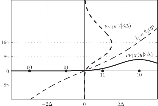
Figure 5.5 PDF (not to scale) of the L-values  obtained as a transformation of the variable
  with PDF
  via the function
  for a 4PAM constellation; here,
We can repeat the same analysis for ![]() . In this case, we have
. In this case, we have

which is shown in Fig. 5.6.
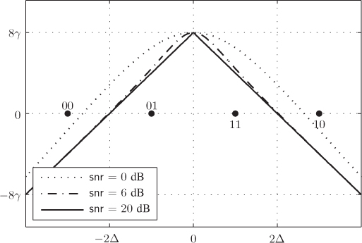
Figure 5.6 Nonlinear relationship  given by (5.15) for a 4PAM constellation
The function ![]() shown in Fig. 5.6 has no inverse, which was essential in deriving the PDF for
shown in Fig. 5.6 has no inverse, which was essential in deriving the PDF for ![]() . To deal with this problem, we tessellate the space of
. To deal with this problem, we tessellate the space of ![]() into two disjoint regions
into two disjoint regions ![]() and
and ![]() such that
such that ![]() , where
, where ![]() and
and ![]() . Over each of the sets, the function
. Over each of the sets, the function ![]() is bijective, and thus, we can define the “pseudoinverse” functions
is bijective, and thus, we can define the “pseudoinverse” functions ![]() and
and ![]() that map
that map ![]() to the values
to the values ![]() with
with ![]() , i.e.,
, i.e., ![]() if
if ![]() .
.
As ![]()
![]() (see Fig. 5.6), we immediately see that the CDF
(see Fig. 5.6), we immediately see that the CDF ![]() for
for ![]() . For
. For ![]() , we obtain
, we obtain

The PDF is now calculated by differentiating (5.16):
where
The negative sign in the second term of (5.17) is a consequence of the differentiation with respect to the lower integration limit of the second term of (5.16). This negative sign is compensated by the negative sign of ![]() with
with ![]() , so only nonnegative functions are added.
, so only nonnegative functions are added.

Figure 5.7 Discontinuous PDF (not to scale) of the L-values  obtained as a transformation of the variable
  with PDF
  via the function
  for a 4PAM constellation; here,
The transformation of the PDF ![]() into the PDF
into the PDF ![]() is shown in Fig. 5.7, where we can observe a “peak” appearing around
is shown in Fig. 5.7, where we can observe a “peak” appearing around ![]() . This is perfectly normal and happens because
. This is perfectly normal and happens because ![]() , see (5.18). The PDF
, see (5.18). The PDF ![]() is thus undefined for
is thus undefined for ![]() .
.
5.1.3 Local Linearization
While it is definitely possible to calculate the PDF of the L-values (as shown in Section 5.1.2), a significant numerical effort may be required, as we do not known the analytical forms of the inverse or pseudoinverse of ![]() . Moreover, such numerical results provide little insight into the properties of BICM systems.
. Moreover, such numerical results provide little insight into the properties of BICM systems.
The problem of finding the PDF of the L-values is greatly simplified when we consider the max-log approximation from (3.99), which reduces the function ![]() to piecewise linear functions. This linearization is typically exploited at the receiver to reduce the complexity of the L-values calculation. Here, we take advantage of the max-log approximation to obtain a piecewise linear model for the L-values. This model will be used in the following sections to develop analytical expressions/approximations for the PDF of the L-values.
to piecewise linear functions. This linearization is typically exploited at the receiver to reduce the complexity of the L-values calculation. Here, we take advantage of the max-log approximation to obtain a piecewise linear model for the L-values. This model will be used in the following sections to develop analytical expressions/approximations for the PDF of the L-values.
The linearization caused by the max-log approximation can be formalized by rewriting the L-values in (3.99) as

where
for ![]() ,
, ![]() and
and ![]() .
.
The tessellation region ![]() in (5.27) contains all the observations
in (5.27) contains all the observations ![]() , for which
, for which ![]() and
and ![]() are the closest (in the sense of Euclidean distance (ED)) symbols to the constellations
are the closest (in the sense of Euclidean distance (ED)) symbols to the constellations ![]() and
and ![]() , respectively. This tessellation principle is valid for any number of dimensions
, respectively. This tessellation principle is valid for any number of dimensions ![]() . We note that although the sum over
. We note that although the sum over ![]() and
and ![]() in (5.26) covers all possible combinations of the indices (i.e., there are
in (5.26) covers all possible combinations of the indices (i.e., there are ![]() sets
sets ![]() ), some of the sets
), some of the sets ![]() are empty.
are empty.
Following the steps we have already taken in (3.51)–(3.53), we express (5.26) as
where ![]() and
and ![]() are given by (3.55) and (3.54), respectively.
are given by (3.55) and (3.54), respectively.
To clarify the definitions above, consider the following example based on the natural binary code (NBC) in Definition 2.11.

Figure 5.8 Tessellation regions  (bottom shaded regions) and
  (top shaded regions) for the NBC in Definition 2.11 and a 4PAM constellation. The piecewise linear functions
  in (5.29) whose pieces are labeled as
  are also shown
The CDF of the L-value ![]() conditioned on the symbol
conditioned on the symbol ![]() can be written using (5.29) as
can be written using (5.29) as
where
Differentiation of (5.31) with respect to ![]() produces the conditional PDF
produces the conditional PDF
where
We also define the set
which is the “image” of ![]() after transformation via
after transformation via ![]() . Of course,
. Of course, ![]() is an interval because it is a linear transformation of the convex set
is an interval because it is a linear transformation of the convex set ![]() , i.e.,
, i.e.,
where
and
are the (normalized by ![]() ) limits of the interval.
) limits of the interval.
5.2 PDF of L-values for 1D Constellations
In this section, we use the linearization procedure presented in Section 5.1.3 and show how to calculate the PDF of the max-log L-values for arbitrary 1D constellations. In this case, the tessellation regions ![]() in (5.27) are intervals (see Fig. 5.8 for an example), i.e.,
in (5.27) are intervals (see Fig. 5.8 for an example), i.e.,
so the limits of the intervals ![]() (5.37) and (5.38) are given by
(5.37) and (5.38) are given by
The following theorem gives a closed-form expression for the conditional PDF of the L-values ![]() for arbitrary 1D constellations.
for arbitrary 1D constellations.
In view of (5.33), each linear function ![]() and the corresponding interval
and the corresponding interval ![]() will “contribute” to the PDF with a piece of a Gaussian function (truncated over the interval
will “contribute” to the PDF with a piece of a Gaussian function (truncated over the interval ![]() , as shown in (5.42)) and whose mean and variance are given by (5.43) and (5.44), respectively. This transformation is illustrated in Fig. 5.9 and is rather intuitive: the Gaussian random variable
, as shown in (5.42)) and whose mean and variance are given by (5.43) and (5.44), respectively. This transformation is illustrated in Fig. 5.9 and is rather intuitive: the Gaussian random variable ![]() , after being transformed via a piecewise linear function
, after being transformed via a piecewise linear function ![]() , has its mean transformed to
, has its mean transformed to ![]() and its variance to
and its variance to ![]() .
.

Figure 5.9 A piecewise linear transformation of a Gaussian PDF  yields a truncated Gaussian function
  . The dotted lines show the extension of the function
  before its truncation and
  marks the solution of
We observe that while the variance of the Gaussian piece in (5.42) depends solely on the distance between the symbols ![]() and
and ![]() defining the tessellation regions
defining the tessellation regions ![]() (see (5.44)), the mean in (5.43) depends also on the symbol
(see (5.44)), the mean in (5.43) depends also on the symbol ![]() . We also note that the limits of the interval
. We also note that the limits of the interval ![]() in (5.35) scale linearly with SNR and so do the mean and the variance in (5.43) and (5.44).
in (5.35) scale linearly with SNR and so do the mean and the variance in (5.43) and (5.44).

Figure 5.10 Tessellation regions  (bottom shaded regions) and
  (top shaded regions) for a 4PAM constellation labeled by BRGC. The piecewise linear functions
  in (5.29) whose pieces are labeled as
  are also shown

Figure 5.11 PDF (not to scale) of the L-values  obtained as a transformation of the variable
  with PDF
  via the function
  based on the max-log approximation for a 4PAM constellation labeled by the BRGC and
  : (a)
: (a)  and (b)
  . The discontinuity of the PDF shown by small white/black circles is due to the piecewise linear form of
  .
.
So far, all the PDFs we have shown were presented to facilitate the understanding of the concept of the linear transformations involved, and thus, are not to scale. In Fig. 5.12, we show the true PDFs ![]() and
and ![]() with
with ![]() and
and ![]() for the exact and max-log L-values. This set of PDFs completely characterize the PDFs
for the exact and max-log L-values. This set of PDFs completely characterize the PDFs ![]() , as
, as ![]() and
and ![]() . The importance of these PDFs is that they fully characterize the L-values of the practically relevant case of a 16QAM constellation labeled by the BRGC shown in Fig. 2.14(b).
. The importance of these PDFs is that they fully characterize the L-values of the practically relevant case of a 16QAM constellation labeled by the BRGC shown in Fig. 2.14(b).

Figure 5.12 PDFs  of the exact L-values (solid lines) and max-log L-values (dashed lines) for a 4PAM constellation labeled by the BRGC and
  : (a)
: (a)  ,
,  , (b)
, (b)  ,
,  , (c)
, (c)  ,
,  , and (d)
  ,
,  . Differences are particularly notable in the vicinity of the borders of the intervals
  , i.e., around
  . The discontinuities of the PDF are shown as small black/white circles. In the case of max-log L-values, they are a consequence of the piecewise linear form of
  , while in the case of exact L-value and
  , the discontinuity is because of the null derivative