
5.4 Fading Channels
Up to now, we considered the case of transmission over fixed-gain channels. To address the problem of finding the distribution of the L-values in fading channels, we define the CDF in (5.31) explicitly conditioned on the SNR, i.e.,
Further, we average the CDF with respect to ![]() , and obtain the PDF of the L-values by differentiating with respect to
, and obtain the PDF of the L-values by differentiating with respect to ![]() , i.e.,
, i.e.,
where, similarly to (5.141), we define
i.e., the dependence of ![]() on the
on the ![]() is made explicit.
is made explicit.
Having changed the order of differentiation and integration, the PDF of the L-values for fading channels in (5.144) and (5.145) is obtained by averaging ![]() over the distribution of the SNR. As we already derived
over the distribution of the SNR. As we already derived ![]() for nonfading channels, we can thus reuse the results from the previous sections. Before presenting the result regarding the PDF of the L-values for fading channels, we introduce a useful lemma.
for nonfading channels, we can thus reuse the results from the previous sections. Before presenting the result regarding the PDF of the L-values for fading channels, we introduce a useful lemma.
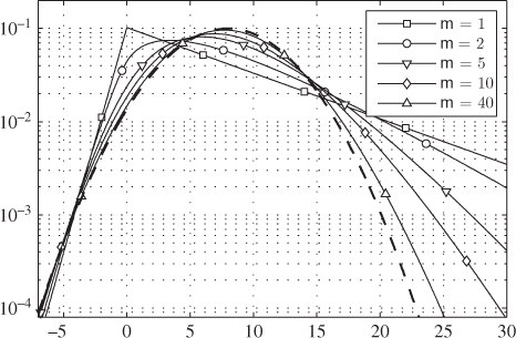
Figure 5.20 PDF of the L-values  for 2PAM in Nakagami-
 fading channel for
  given by (5.165) and (5.166). The thick dashed line indicates the PDF of the L-values for the AWGN channel with
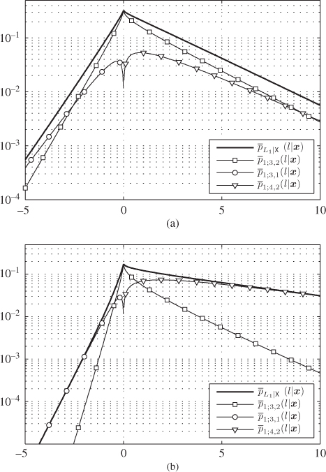
Figure 5.21 PDF of the L-values for 4PAM labeled by the BRGC over a Rayleigh fading channel and the PDF pieces  for
for  : (a)
: (a)  and (b)
5.5 Gaussian Approximations
Although, as explained in the previous sections, we can find the PDF through the explicit derivation of the CDF, such an approach has two main disadvantages: (i) the expressions require analysis of the tessellation space and (ii) the resulting forms are piecewise functions. The former is critical when we have to deal with arbitrary constellations, particularly when the dimensionality of the signal space increases beyond ![]() . The latter complicates the analysis of the operations on the PDFs. For example, recall that the maximum likelihood (ML) decoderadds L-values, and thus, to characterize the performance of the decoder, we need to be able to find the CDF of the sum of L-values. This in turn requires finding the convolution of the PDFs and the integration of its tail,10 which becomes difficult for PDFs defined via piecewise functions.
. The latter complicates the analysis of the operations on the PDFs. For example, recall that the maximum likelihood (ML) decoderadds L-values, and thus, to characterize the performance of the decoder, we need to be able to find the CDF of the sum of L-values. This in turn requires finding the convolution of the PDFs and the integration of its tail,10 which becomes difficult for PDFs defined via piecewise functions.
The main objective of this section is to provide a model for the PDF of the L-values, such that (i) its parameters are easy to find, (ii) its form simplifies operations on the PDF of the L-values (such as convolution), and (iii) the integration over its tail accurately estimates the actual value of the probability of error.
Assuming that the L-values are Gaussian is convenient because it will, indeed, simplify the operations of convolution (necessary to find the PDF of the sum of the L-values) and integration (necessary to find the error probability). The Gaussian model is also interesting because the expression we derived for nonfading channels already contains Gaussian pieces whose parameters (mean and variance) depend in closed form on the constellation and labeling. The main idea is thus to take only the Gaussian piece from the piecewise model and to ignore windowing and weighting (correction) factors. The resulting simplicity is indeed appealing and, in such a case, the corresponding approximate PDF conditioned on a transmitted symbol will be
where the mean and variance are the parameters related to a Gaussian piece ![]() , indexed by
, indexed by ![]() and
and ![]() , i.e.,
, i.e.,
where ![]() and
and ![]() are given by (5.43) and (5.44), respectively. The main problem consists then in finding the indices
are given by (5.43) and (5.44), respectively. The main problem consists then in finding the indices ![]() and
and ![]() such that (5.167) represents “well” the PDF
such that (5.167) represents “well” the PDF ![]() .
.
We continue to keep in mind that the particular choice of ![]() and
and ![]() should be assessed using the criterion related to the objective we fixed, namely, an the accurate evaluation of the integration over the tails of the PDF. As the details on the performance evaluation of BICM receivers are mostly given in Chapter 6, here, we will only highlight the most important features of the two proposed heuristics with respect to their impact on the accuracy of evaluation of the BEP for uncoded transmission. While passing through Section 6.1 may be helpful, the following contents can be understood without such additional reading.
should be assessed using the criterion related to the objective we fixed, namely, an the accurate evaluation of the integration over the tails of the PDF. As the details on the performance evaluation of BICM receivers are mostly given in Chapter 6, here, we will only highlight the most important features of the two proposed heuristics with respect to their impact on the accuracy of evaluation of the BEP for uncoded transmission. While passing through Section 6.1 may be helpful, the following contents can be understood without such additional reading.
5.5.1 Consistent Model
For notational convenience, we will denote the transmitted symbol by ![]() and assume that it belongs to the subconstellation
and assume that it belongs to the subconstellation ![]() , i.e.,
, i.e., ![]() is the value of the
is the value of the ![]() th bit in the label
th bit in the label ![]() , (
, (![]() , see Section 2.5.2). The next definition introduces the first Gaussian model for the PDF of the L-values, namely, the so-called consistent model (CoM).
, see Section 2.5.2). The next definition introduces the first Gaussian model for the PDF of the L-values, namely, the so-called consistent model (CoM).
Definition 5.15 states that the tessellation region ![]() that provides the most “representative” Gaussian piece (i.e., the one whose parameters will be used for the approximation in (5.167)) is obtained by considering the transmitted symbol
that provides the most “representative” Gaussian piece (i.e., the one whose parameters will be used for the approximation in (5.167)) is obtained by considering the transmitted symbol ![]() and the closest symbol from
and the closest symbol from ![]() . From (5.43), we know that
. From (5.43), we know that
and
Using (5.174) and (5.175) in (5.168) and (5.169), we conclude that for any ![]() ,
,
where
is the distance between ![]() and the closest symbol having a different bit at position
and the closest symbol having a different bit at position ![]() . Therefore, (5.167) becomes
. Therefore, (5.167) becomes
which has the same form we would obtain for a 2PAM constellation if we used ![]() and
and ![]() in (5.52).
in (5.52).
The PDF in (5.179) also satisfies the consistency condition in Definition 3.8. This particular property explains the name we gave to the model that also corresponds to decomposing the BICM into “virtual” 2PAM transmissions, each characterized by the distance between the corresponding virtual 2PAM symbols.

Figure 5.22 PDF of the L-values  and its approximations based on the CoM
  and ZcM
  for an 8PSK constellation labeled by the BRGC and two SNR values: (a)
  and (b)

Figure 5.23 PDF of the L-values  for
for  and its approximations for an 8PSK constellation labeled by the BRGC and two SNR values. In this case,
Let us now verify how the obtained models affect the calculation of the BEP, which is an important parameter characterizing digital communications.11 Here, the BEP for uncoded transmission in (3.110) can be obtained directly from the definition of the L-value.
where
is the BEP conditioned on the transmitted symbol ![]() .
.
For the case in Example 5.16, using the approximate PDF in (5.183), we obtain ![]() and
and ![]() , and from (5.184), we obtain
, and from (5.184), we obtain ![]() . Thus,
. Thus,
We note that the expressions in (5.190) and (5.191) are similar to the exact error probability expressions given in (6.58) and (6.60), respectively. Although the dominant Q-function ![]() correctly appear in the expressions derived using the CoM, differences appears when other terms are compared. We also note that for sufficiently high SNR,
correctly appear in the expressions derived using the CoM, differences appears when other terms are compared. We also note that for sufficiently high SNR, ![]() . Thus, depending on the position
. Thus, depending on the position ![]() , the transmitted bits are more (or less) prone to errors. This so-called unequal error protection (UEP) will be analyzed in Chapter 8.
, the transmitted bits are more (or less) prone to errors. This so-called unequal error protection (UEP) will be analyzed in Chapter 8.
For the case in Example 5.17, we obtain
The first (dominating) terms in (5.192) and (5.193) are again the same as the dominating terms in the exact expressions (6.65) and (6.66), and the differences appear only in the remaining terms.
Finally, it interesting to analyze the CoM at high SNR. When ![]() ,
, ![]() is increasingly narrow and centered around
is increasingly narrow and centered around ![]() . After the transformation
. After the transformation ![]() , the L-values are most likely to lie in the vicinity of
, the L-values are most likely to lie in the vicinity of ![]() . In other words, for high SNR,
. In other words, for high SNR, ![]() is centered around
is centered around ![]() and the components
and the components ![]() for
for ![]() or
or ![]() vanish. This is in fact what is observed in Figs. 5.22 and 5.23 for
vanish. This is in fact what is observed in Figs. 5.22 and 5.23 for ![]() , i.e., the CoM approximates well the true PDF around its mean value. This observation has often been used as a justification to use the CoM to approximate the PDF of the L-values.
, i.e., the CoM approximates well the true PDF around its mean value. This observation has often been used as a justification to use the CoM to approximate the PDF of the L-values.
5.5.2 Zero-Crossing Model
For any ![]() , the conditional BEP in (5.189) can be expressed as
, the conditional BEP in (5.189) can be expressed as
which shows that to have a good approximation of the conditional BEP, an accurate model of the tail of the PDF is necessary. When observing the results obtained with the CoM (see e.g., Fig. 5.22 (b)), we note that the (left) tail of the PDF is not well approximated. Consequently, the second terms in the BEP expressions obtained in Examples 5.16 and 5.17 do not match the terms that appear in the exact evaluation.
In this section, we introduce the zero-crossing model (ZcM) which aims at approximating the PDF well around ![]() , and thus, removing some of the discrepancies (in terms of BEP) observed when using the CoM. Before giving a formal definition, we introduce this model using an example. Consider an 8PSK constellation labeled by the BRGC,
, and thus, removing some of the discrepancies (in terms of BEP) observed when using the CoM. Before giving a formal definition, we introduce this model using an example. Consider an 8PSK constellation labeled by the BRGC, ![]() ,
, ![]() , and
, and ![]() . The exact PDF and the CoM approximation are shown in Fig. 5.24, where the shaded regions represent the integral in (5.194). This figure clearly shows that the CoM approximation fails to predict well the conditional BEP in (5.194). On the other hand, this figure also shows the ZcM defined below, which uses the Gaussian piece around
. The exact PDF and the CoM approximation are shown in Fig. 5.24, where the shaded regions represent the integral in (5.194). This figure clearly shows that the CoM approximation fails to predict well the conditional BEP in (5.194). On the other hand, this figure also shows the ZcM defined below, which uses the Gaussian piece around ![]() . This results in a PDF that approximates much better the tail of the exact PDF, and thus, the conditional BEP in (5.194).
. This results in a PDF that approximates much better the tail of the exact PDF, and thus, the conditional BEP in (5.194).

Figure 5.24 PDF of the L-values  and its approximations based on the CoM
  and ZcM
  for an 8PSK constellation labeled by the BRGC,
  and
and  . The shaded regions represent the conditional BEP in (5.194)
We can now compare the ZcM in Definition 5.18 with the CoM in Definition 5.15. First of all, we see that both ZcM and CoM require finding the symbol from ![]() which is closest to
which is closest to ![]() . This symbol (and the corresponding index) are thus common in both models. The difference is how to determine the complementary index
. This symbol (and the corresponding index) are thus common in both models. The difference is how to determine the complementary index ![]() (when
(when ![]() ) or
) or ![]() (when
(when ![]() ). In Definition 5.15, this index is simply taken as equal to
). In Definition 5.15, this index is simply taken as equal to ![]() , while in Definition 5.18, we perform a search over
, while in Definition 5.18, we perform a search over ![]() to find
to find ![]() closest to
closest to ![]() . In some cases, both definitions yield exactly the same results, namely, when the symbols
. In some cases, both definitions yield exactly the same results, namely, when the symbols ![]() and
and ![]() belong to the tessellation region
belong to the tessellation region ![]() they define, i.e.,
they define, i.e., ![]() . In these cases, the PDF conditioned on
. In these cases, the PDF conditioned on ![]() or
or ![]() obtained from ZcM and CoM will be same.
obtained from ZcM and CoM will be same.
Similarly to (5.190) and (5.191), now that we have the ZcM PDF of the L-values for 4PAM labeled by the BRGC in (5.197) and (5.198), we can calculate the BEP. As we have already stated in Example 5.19, the only difference with the CoM occurs for ![]() and
and ![]() , where we have
, where we have ![]() and then we obtain
and then we obtain
Again we compare the expressions in (5.201) and (5.202) with the exact expression in (6.58) and (6.60). Unlike in the CoM case, for the ZcM, the error probability for ![]() coincides with the exact calculation. For
coincides with the exact calculation. For ![]() , the result is the same as in (5.191).
, the result is the same as in (5.191).
5.5.3 Fading Channels
The extension of the developed formulas to the case of the fading channel may be done by averaging the approximate Gaussian PDF in (5.167) over the distribution of the fading
In the particular case of Rayleigh fading, using the same approach as those leading to (5.160), we obtain

where ![]() and
and ![]() depend also on the Gaussian simplification strategy (CoM vs. ZcM).
depend also on the Gaussian simplification strategy (CoM vs. ZcM).

Figure 5.25 PDF of the L-values for a 4PAM constellation labeled by the BRGC in Rayleigh fading channel and  . The exact expression
  and the approximations via the ZcM
  and the CoM
  for
for  are shown for (a)
  and (b)
5.5.4 QAM and PSK Constellations
Two of the most practically relevant constellations are the ![]() PAM and
PAM and ![]() PSK constellations labeled by the BRGC. In these cases, it is possible to determine the forms of the approximate PDF without algorithmic steps. This is thanks to the structure of the binary labeling as well as to the regular geometry of the constellation. In other words, in these cases we are able to determine the parameters of the approximate PDF (i.e., the indices
PSK constellations labeled by the BRGC. In these cases, it is possible to determine the forms of the approximate PDF without algorithmic steps. This is thanks to the structure of the binary labeling as well as to the regular geometry of the constellation. In other words, in these cases we are able to determine the parameters of the approximate PDF (i.e., the indices ![]() and
and ![]() of the representative tessellation regions
of the representative tessellation regions ![]() ) as a function of the index
) as a function of the index ![]() of the transmitted symbol
of the transmitted symbol ![]() .
.
We start by considering the BRGC for 16PAM shown in Fig. 5.26. We note that for a given ![]() , the constellation may be split into
, the constellation may be split into ![]() groups of
groups of ![]() consecutive symbols. These groups are identified by rectangles on the left-hand side (l.h.s.) of Fig. 5.26. Furthermore, because of the symmetry of the labeling, it is enough to consider the PDF conditioned on
consecutive symbols. These groups are identified by rectangles on the left-hand side (l.h.s.) of Fig. 5.26. Furthermore, because of the symmetry of the labeling, it is enough to consider the PDF conditioned on ![]() , which implies that only the symbols
, which implies that only the symbols ![]() are relevant for the analysis. For any symbol
are relevant for the analysis. For any symbol ![]() within each group, the closest symbol from
within each group, the closest symbol from ![]() lies also within the group. Because of the symmetries of the constellation, it is enough to analyze the first group, shown as shaded rectangles in Fig. 5.26.
lies also within the group. Because of the symmetries of the constellation, it is enough to analyze the first group, shown as shaded rectangles in Fig. 5.26.

Figure 5.26 Tessellation regions for a 16PAM constellation labeled by the BRGC. The shaded rectangles gather the symbols that are relevant for the PDF computation. The subconstellations  and
and  are indicated by white and black circles, respectively, and the tessellation regions that define the zero-crossing for the relevant group of bits are shown by a thick line
To obtain the CoM, we note that for any ![]() (because we analyze
(because we analyze ![]() , it follows that
, it follows that ![]() ), the closest symbol from
), the closest symbol from ![]() is
is ![]() (e.g., we have
(e.g., we have ![]() for
for ![]() ,
, ![]() for
for ![]() , etc.). The distance between the symbols is given
, etc.). The distance between the symbols is given ![]() , so we obtain
, so we obtain
By using (5.210) in (5.179), we obtain the CoM PDF for an ![]() PAM constellation labeled by the BRGC, namely, for any
PAM constellation labeled by the BRGC, namely, for any ![]() (
(![]() ),
),
Similarly, in the case of the ZcM, it is enough to characterize the PDF of the symbols within the first group we identified because the closest “zero-crossing” tessellation region ![]() is also defined by the symbols from the same group. These regions are shown as thick lines in Fig. 5.26. Namely, for
is also defined by the symbols from the same group. These regions are shown as thick lines in Fig. 5.26. Namely, for ![]() , we easily find
, we easily find ![]() and
and ![]() ; for
; for ![]() , we obtain
, we obtain ![]() and
and ![]() ; and so on; then, we also find
; and so on; then, we also find ![]() . More generally, for any
. More generally, for any ![]() ,
, ![]() and
and ![]() . Thus, for any
. Thus, for any ![]() in the group and
in the group and ![]() , we find from the relations (5.43) and (5.44) that
, we find from the relations (5.43) and (5.44) that
where (5.212) follows from using ![]() . Using (5.212) and (5.213) in (5.167) gives
. Using (5.212) and (5.213) in (5.167) gives
The results in (5.211) and (5.214) are summarized in Table 5.1.
Table 5.1 ![]() PAM constellations labeled by the BRGC: parameters
PAM constellations labeled by the BRGC: parameters ![]() and
and ![]() defining the Gaussian PDF in (5.167) for
defining the Gaussian PDF in (5.167) for ![]() (i.e.,
(i.e., ![]() )
)
| Gaussian Model | ||
| CoM | ||
| ZcM |
The case of ![]() PSK shown in Fig. 5.27 may be treated in a similar way. The main difference is that the L-value
PSK shown in Fig. 5.27 may be treated in a similar way. The main difference is that the L-value ![]() and
and ![]() will have the same distribution because the groups of the symbols for
will have the same distribution because the groups of the symbols for ![]() and
and ![]() have the same form due to the circular symmetry of the constellation, i.e., the first and the last symbols (
have the same form due to the circular symmetry of the constellation, i.e., the first and the last symbols (![]() and
and ![]() in Fig. 5.27) become adjacent. It is thus enough to calculate the parameters of the simplified form of the PDF for
in Fig. 5.27) become adjacent. It is thus enough to calculate the parameters of the simplified form of the PDF for ![]() and consider only symbol
and consider only symbol ![]() , i.e.,
, i.e., ![]() . Again, for the CoM, we have
. Again, for the CoM, we have ![]() and
and ![]() , so from (5.135), we obtain
, so from (5.135), we obtain ![]() . For the ZcM, we use
. For the ZcM, we use ![]() and
and ![]() and thus
and thus ![]() and from (5.132), we get
and from (5.132), we get

Figure 5.27 Tessellation regions  , for a 16PSK constellation labeled by the BRGC. The subconstellations
  and
and  are indicated by white and black circles, respectively, and the regions
  in which the zero-crossing occurs are shaded: (a)
  , (b)
, (b)  , (c)
, (c)  , and (d)
These results are summarized in Table 5.2.
5.6 Bibliographical Notes
The idea of the BICM channel can be tracked to [1], where the model from Fig. 5.2 corresponds to the model in [1, Fig. 3]. The model in Fig. 5.1 corresponds to the one introduced and formalized later in [2, Fig. 1]. The statistics of the L-values for the performance evaluation have been used in various works, e.g., in [1–4]. The formalism of using the PDF to evaluate the performance of the decoder in BICM transmissions was introduced in [5]. A probabilistic description of the L-values was also considered for the analysis of the decoding in turbo codes (TCs), low-density parity-check (LDPC) codes, or turbo-like processing in [6–8], respectively.
The probabilistic model for the L-values and 2PAM is well known [6 8, 9]. The explicit modeling of the PDF for BICM based on quadrature amplitude modulation (QAM) constellations appeared in [10–13], for phase shift keying (PSK) constellations labeled by the BRGC in [14], and for the case of arbitrary 2D constellations in [15 16]. The effect of fading on the PDF of L-values was shown for 2PAM in [2 6], for ![]() PAM in [17–19], and for 2D constellations in [20]. The probabilistic modeling of the L-values has also been considered in relay channels [21], and in multiple-input multiple-output (MIMO) transmission [22].
PAM in [17–19], and for 2D constellations in [20]. The probabilistic modeling of the L-values has also been considered in relay channels [21], and in multiple-input multiple-output (MIMO) transmission [22].
The Gaussian model of the L-values is well known and has been applied in [23]. The CoM defined in Section 5.5.1 has been used in [24] while the ZcM defined in Section 5.5.2 was proposed in [10 11], formalized in [12], and extended to the case of nonequidistant constellations in [25]. The ZcM has been recently used in [26] to study the asymptotic optimality of bitwise (BICM) decoders.
The space tessellation discussed in Section 5.3.1, based on solving the set of inequalities in (5.72), exploits the well-known duality between the line and points description [27, Chapter 8.2]. For details of finding a convex hull, we refer the reader to [27, Chapter 1.1], [28, Sec. 2.10]. The description of a method to find the vertices of the hull may be found in [28, Sec. 2.12].
References
- [1] Caire, G., Taricco, G., and Biglieri, E. (1998) Bit-interleaved coded modulation. IEEE Trans. Inf. Theory, 44 (3), 927–946.
- [2] Martinez, A., Guillén i Fàbregas, A., and Caire, G. (2006) Error probability analysis of bit-interleaved coded modulation. IEEE Trans. Inf. Theory, 52 (1), 262–271.
- [3] Biglieri, E., Caire, G., Taricco, G., and Ventura-Traveset, J. (1996) Simple method for evaluating error probabilities. Electron. Lett., 32 (2), 191–192.
- [4] Biglieri, E., Caire, G., Taricco, G., and Ventura-Traveset, J. (1998) Computing error probabilities over fading channels: a unified approach. Eur. Trans. Telecommun., 9 (1), 15–25.
- [5] Abedi, A. and Khandani, A. K. (2004) An analytical method for approximate performance evaluation of binary linear block codes. IEEE Trans. Commun., 52 (2), 228–235.
- [6] ten Brink, S. (2001) Convergence behaviour of iteratively decoded parallel concatenated codes. IEEE Trans. Commun., 49 (10), 1727–1737.
- [7] Fossorier, M. P. C., Lin, S., and Costello, D.J. Jr. (1999) On the weight distribution of terminated convolutional codes. IEEE Trans. Inf. Theory, 45 (5), 1646–1648.
- [8] Tüchler, M. (2004) Design of serially concatenated systems depending on the block length. IEEE Trans. Commun., 52 (2), 209–218.
- [9] Papke, L., Robertson, P., and Villebrun, E. (1996) Improved decoding with the SOVA in a parallel concatenated (turbo-code) scheme. IEEE International Conference on Communications (ICC), June 1996, Dallas, TX.
- [10] Benjillali, M., Szczecinski, L., and Aissa, S. (2006) Probability density functions of logarithmic likelihood ratios in rectangular QAM. 23rd Biennial Symposium on Communications, May 2006, Kingston, ON, Canada
- [11] Benjillali, M., Szczecinski, L., Aissa, S., and Gonzalez, C. (2008) Evaluation of bit error rate for packet combining with constellation rearrangement. Wiley J Wirel Commun. Mob. Comput., 8, 831–844.
- [12] Alvarado, A., Szczecinski, L., Feick, R., and Ahumada, L. (2009) Distribution of L-values in Gray-mapped
 -QAM: closed-form approximations and applications. IEEE Trans. Commun., 57 (7), 2071–2079.
 - [13] Alvarado, A., Szczecinski, L., and Feick, R. (2007) On the distribution of extrinsic L-values in gray-mapped 16-QAM. AMC International Wireless Communications and Mobile Computing Conference (IWCMC), August 2007, Honolulu, HI.
- [14] Szczecinski, L. and Benjillali, M. (2006) Probability density functions of logarithmic likelihood ratios in phase shift keying BICM. IEEE Global Telecommunications Conference (GLOBECOM), November 2006, San Francisco, CA.
- [15] Szczecinski, L., Bettancourt, R., and Feick, R. (2006) Probability density function of reliability metrics in BICM with arbitrary modulation: closed-form through algorithmic approach. IEEE Global Telecommunications Conference (GLOBECOM), November 2006, San Francisco, CA.
- [16] Szczecinski, L., Bettancourt, R., and Feick, R. (2008) Probability density function of reliability metrics in BICM with arbitrary modulation: closed-form through algorithmic approach. IEEE Trans. Commun., 56 (5), 736–742.
- [17] Szczecinski, L., Alvarado, A., and Feick, R. (2007) Probability density functions of reliability metrics for 16-QAM-based BICM transmission in Rayleigh channel. IEEE International Conference on Communications (ICC), June 2007, Glasgow, UK.
- [18] Szczecinski, L., Alvarado, A., and Feick, R. (2009) Distribution of max-log metrics for QAM-based BICM in fading channels. IEEE Trans. Commun., 57 (9), 2558–2563.
- [19] Szczecinski, L., Xu, H., Gao, X., and Bettancourt, R. (2007) Efficient evaluation of BER for arbitrary modulation and signaling in fading channels. IEEE Trans. Commun., 55 (11), 2061–2064.
- [20] Kenarsari-Anhari, A. and Lampe, L. (2010) An analytical approach for performance evaluation of BICM over Nakagami-
 fading channels. IEEE Trans. Commun., 58 (4), 1090–1101.
 - [21] Benjillali, M. and Szczecinski, L. (2010) Detect-and-forward in two-hop relay channels: a metrics-based analysis. IEEE Trans. Commun., 58 (6), 1729–1732.
- [22] Čirkić, M., Persson, D., Larsson, J., and Larsson, E. G. (2012) Approximating the LLR distribution for a class of soft-output mimo detectors. IEEE Trans. Signal Process., 60 (12), 6421–6434.
- [23] Guillén i Fàbregas, A., Martinez, A., and Caire, G. (2004) Error probability of bit-interleaved coded modulation using the Gaussian approximation. Conference on Information Sciences and Systems (CISS), March 2004, Princeton University, NJ.
- [24] Hermosilla, C. and Szczecinski, L. (2005) Performance evaluation of linear turbo-receivers using analytical extrinsic information transfer functions. EURASIP J. Appl. Signal Process., 2005 (6), 892–905.
- [25] Hossain, Md.J., Alvarado, A., and Szczecinski, L. (2011) Towards fully optimized BICM transceivers. IEEE Trans. Commun., 59 (11), 3027–3039.
- [26] Ivanov, M., Alvarado, A., Brännström, F., and Agrell, E. (2014) On the asymptotic performance of bit-wise decoders for coded modulation. IEEE Trans. Inf. Theory, 60 (5), 2796–2804.
- [27] de Berg, M., van Kreveld, M., Overmars, O., and Schwartzkopf, O. (2000) Computational Geometry, Algorithms and Applications, Springer.