
Chapter 7
Correction of L-values
The L-values are the signals/messages exchanged in bit-interleaved coded modulation (BICM) receivers. We saw in Chapter 3 that, thanks to the formulation of the L-values in the logarithm domain, multiplication of probabilities/likelihoods transforms into addition of the corresponding L-values. This makes the L-values well suited for numerical implementation. Furthermore, the L-values can be processed in abstraction of how they were calculated. The designer can then connect well-defined processing blocks, which is done under the assumption that the L-values can be transformed into probabilities/likelihoods. This assumption does not hold in all cases, as the L-values might have been incorrectly calculated, resulting in mismatched L-values. In this chapter, we take a closer look at the problem of how to deal with this mismatch.
We will discuss the motivation for L-values correction in Section 7.1 and explain optimal processing rules in Section 7.2. Suboptimal (linear) correction strategies will be studied in Section 7.3.
7.1 Mismatched Decoding and Correction of L-values
As discussed in Section 3.2, the BICM decoding rule
is solely based on the L-values ![]() calculated as
calculated as
Thus, decoding is carried out in abstraction of the channel model, i.e., the L-values are assumed to carry all the information necessary for decoding.
We also know from Section 3.2 that the decoding rule (7.1) is suboptimal. More specifically, the decoding metric in (7.1) implicitly uses the following approximation:
where, using (3.38), we have
We showed in Example 3.3 that (7.3) may hold with equality in some particular cases, but in general, the decoding metric used by (7.1) is mismatched. As we explained in Section 3.2, an achievable rate for the (mismatched) BICM decoder is then given by the generalized mutual information (GMI).
In previous chapters, the analysis of the BICM decoder in (7.1) was done assuming (7.2) is implemented. In this chapter, however, we are interested in cases when (7.2) is no applied exactly, i.e., when the L-values are incorrectly calculated, or–in other words–when they are mismatched. We emphasize that this mismatch comes on the top of the mismatch caused by the suboptimal decoding rule (7.1).
The main reasons for the L-values to be mismatched are the following:
- Modeling Errors: The model used to derive
 is not accurate. For example, if the actual distribution of the additive noise
  is ignored (e.g., when
  is not Gaussian). Similarly, the parameters of the distributions might have been incorrectly estimated. This is, in fact, almost always the case in practice, as estimation implies unavoidable estimation errors.
 - Simplifications: The L-values are calculated using simplifications introduced to diminish the computational load. This includes the popular max-log approximation as well as other methods discussed in Section 3.3.3. Approximations are in fact, unavoidable in interference-limited transmission scenarios, where the effective constellation size grows exponentially with the number of data streams (which corresponds, e.g., to the number of transmitting antennas in multiple-input multiple-output (MIMO) systems).
- L-values Processing: After the L-values are calculated (possibly with modeling errors and simplifications), some extra operations may be necessary to render them suitable for decoding. This may include quantization, truncation, scaling, or any other operation directly applied on the L-values.
In the first two cases above, the likelihoods ![]() are incorrectly calculated. Formally, we assume that the decoder uses
are incorrectly calculated. Formally, we assume that the decoder uses ![]() instead of
instead of ![]() . The binary decoder remains unaware of the mismatch and will blindly use the former. The mismatched metric is then
. The binary decoder remains unaware of the mismatch and will blindly use the former. The mismatched metric is then ![]() . In analogy to (4.30)–(4.33), we have that the BICM decoding rule in this case is
. In analogy to (4.30)–(4.33), we have that the BICM decoding rule in this case is
We can now define mismatched L-values as
where ![]() is a mismatched demapper.
is a mismatched demapper.
Transforming (7.6) into
we obtain again a form similar to (7.1), i.e., the decoder remains unaware of the mismatch and blindly uses the mismatched L-values ![]() . Moreover, because (7.5) and (7.8) are equivalent, we know now that the mismatch in the likelihoods translates into an equivalent mismatch in the L-values. Thus, from now on, we do not analyze the source of the mismatch, and we uniquely consider the mismatched L-values calculated by the mismatched demapper
. Moreover, because (7.5) and (7.8) are equivalent, we know now that the mismatch in the likelihoods translates into an equivalent mismatch in the L-values. Thus, from now on, we do not analyze the source of the mismatch, and we uniquely consider the mismatched L-values calculated by the mismatched demapper ![]() defined in (7.6). This is also convenient because our considerations will be done in the domain of the L-values, so from now on we will avoid references to the observations
defined in (7.6). This is also convenient because our considerations will be done in the domain of the L-values, so from now on we will avoid references to the observations ![]() . Instead, we consider the mismatched L-values as the outputs of an equivalent channel, shown in Fig. 7.1, which encompasses the actual transmission and the mismatched demapping.
. Instead, we consider the mismatched L-values as the outputs of an equivalent channel, shown in Fig. 7.1, which encompasses the actual transmission and the mismatched demapping.
Owing to the memoryless property of the channel, the BICM decoding rule based on the mismatched L-values ![]() can be again written as
can be again written as
where ![]() is used to denote the metric defined for the equivalent channel outputs, i.e., a metric based on the mismatched L-values rather than on the channel observations. We know from Section 3.1 that the metric
is used to denote the metric defined for the equivalent channel outputs, i.e., a metric based on the mismatched L-values rather than on the channel observations. We know from Section 3.1 that the metric ![]() is optimal in the sense of minimizing the probability of decoding error. However, we want to preserve the bitwise operation, so we will prefer the suboptimal decoding
is optimal in the sense of minimizing the probability of decoding error. However, we want to preserve the bitwise operation, so we will prefer the suboptimal decoding
where we decomposed the metric ![]() into a product of bitwise metrics
into a product of bitwise metrics ![]() , i.e.,
, i.e.,
where ![]() .
.

Figure 7.1 The mismatched L-values  are the result of a mismatched demapping and can be corrected using (a) scalar or (b) multidimensional functions
  . These functions act as demappers for the equivalent channel (shown as a shaded rectangle), which concatenates the actual transmission channel (with output
  ) and the mismatched demapper
We can now develop (7.10) along the lines of (7.7) and (7.8); namely,
where
Thus, treating ![]() as the outcome of the equivalent channel,
as the outcome of the equivalent channel, ![]() has a meaning of a new L-value calculated on the basis of the metrics
has a meaning of a new L-value calculated on the basis of the metrics ![]() .
.
The decoding results will clearly change depending on the choice of the decoding metric ![]() . In particular, using
. In particular, using ![]() with
with
and ![]() being an arbitrary nonzero function independent of
being an arbitrary nonzero function independent of ![]() , we obtain the relationship
, we obtain the relationship ![]() from (7.14). In other words, by using
from (7.14). In other words, by using ![]() , we guarantee that (7.13) and (7.8) are equivalent. This means that the decoder using the observations
, we guarantee that (7.13) and (7.8) are equivalent. This means that the decoder using the observations ![]() and the metrics
and the metrics ![]() carries out the same operation as the decoder using the observations
carries out the same operation as the decoder using the observations ![]() and the metrics
and the metrics ![]() . Using such a metric, we actually assume that the relationship (7.4) holds,1 and thus, we ignore the fact that
. Using such a metric, we actually assume that the relationship (7.4) holds,1 and thus, we ignore the fact that ![]() is mismatched.
is mismatched.
On the other hand, if we are aware of the presence of the mismatch, i.e., if we know that (7.4) does not hold, we should use a different metric ![]() . This implies a different form of the function
. This implies a different form of the function ![]() , which is meant to “correct” the effect of the mismatch. This is the focus of this chapter. From this perspective, the metric
, which is meant to “correct” the effect of the mismatch. This is the focus of this chapter. From this perspective, the metric ![]() in (7.15) is “neutral” as it does lead to the trivial correction
in (7.15) is “neutral” as it does lead to the trivial correction ![]() .
.
We say that the correction is multidimensional if it follows the general formulation in (7.14) and depends on a vector ![]() . We say a correction is scalar if the
. We say a correction is scalar if the ![]() th corrected L-value is obtained using only the corresponding mismatched L-value, i.e.,
th corrected L-value is obtained using only the corresponding mismatched L-value, i.e., ![]() . Then, the correction function takes the form
. Then, the correction function takes the form
These two correction strategies are illustrated in Fig. 7.1.
A linear correction (scaling) completely removes the effect of the mismatch in Example 7.1. In general, however, we cannot always guarantee that the corrected L-values ![]() are identical to
are identical to ![]() . In the following example, we explore the possibility of using multidimensional correction functions.
. In the following example, we explore the possibility of using multidimensional correction functions.
While multidimensional correction functions can offer advantages (as shown in Example 7.2), their main drawback with respect to their scalar counterpart is that they are, in general, more complex to implement and to design. This is important when the mismatch is a result of a simplified processing introduced for complexity reduction. In this situation, the correction of the mismatch should also have low complexity. This is why scalar correction is an interesting alternative. Such a scalar correction, which neglects the relationship between the L-values ![]() is, in fact, well aligned with the spirit of BICM where all the operations are done at a bit level.
is, in fact, well aligned with the spirit of BICM where all the operations are done at a bit level.
In this chapter, we take a general view on the problem of correcting L-values and focus on finding suitable scalar correction strategies for the mismatched L-values. There are two issues to consider. The first one is of a fundamental nature: what is an optimal correction strategy? The second relates to practical implementation aspects: what are good simplified (and thus suboptimal) correction strategies? As we will see in this chapter, an optimal correction function ![]() can be defined but is in general nonlinear, and thus, its implementation may be cumbersome. This will lead us to mainly focus on (suboptimal) linear corrections.
can be defined but is in general nonlinear, and thus, its implementation may be cumbersome. This will lead us to mainly focus on (suboptimal) linear corrections.
7.2 Optimal Correction of L-values
The assumption that the corrected L-values ![]() will be used by the decoder defined in (7.13) leads to the obvious question: how is the decoder affected by the mismatch? Once this question is answered, we may design correction strategies aiming at improving the decoder'sperformance.
will be used by the decoder defined in (7.13) leads to the obvious question: how is the decoder affected by the mismatch? Once this question is answered, we may design correction strategies aiming at improving the decoder'sperformance.
7.2.1 GMI-Optimal Correction
From an information-theoretic point of view, considering the effect of the mismatched L-values on the performance of a BICM decoder in (7.13) is similar to the problem of analyzing the mismatched decoding metric in a BICM decoder, as we did in Section 4.3.1. The main difference now is that the decoder in (7.10) uses the metrics ![]() calculated for the outputs of the equivalent channel
calculated for the outputs of the equivalent channel ![]() . As the decoding (7.10) has the form of the BICM decoder, an achievable rate, in this case, can also be characterized by the GMI, i.e.,
. As the decoding (7.10) has the form of the BICM decoder, an achievable rate, in this case, can also be characterized by the GMI, i.e.,
where, thanks to (7.11), we used Theorem 4.11 to express the GMI as the sum of bitwise GMIs, which are defined in the same way as in (4.47), i.e.,
To pass from (7.20) to (7.21), we used the scalar correction principle, i.e., ![]() . Using (7.22) in (7.19) yields
. Using (7.22) in (7.19) yields
The GMI in (7.23) is an achievable rate for the decoder in (7.13), which uses the observations ![]() and applies scalar correction functions. The scalar correction assumption remains implicit throughout the rest of this chapter.
and applies scalar correction functions. The scalar correction assumption remains implicit throughout the rest of this chapter.
Clearly, using the “neutral” metric ![]() in (7.15) corresponds to feeding the decoder with the mismatched, uncorrected L-values
in (7.15) corresponds to feeding the decoder with the mismatched, uncorrected L-values ![]() , so the achievable rates are not changed when compared to those obtained by decoding on the basis of
, so the achievable rates are not changed when compared to those obtained by decoding on the basis of ![]() and the metrics
and the metrics ![]() . Theorem 7.3 is provided here to connect the analysis based on the metrics
. Theorem 7.3 is provided here to connect the analysis based on the metrics ![]() and the analysis of the performance based on the metrics
and the analysis of the performance based on the metrics ![]() .
.
As the GMI is suitable to assess the performance of BICM receivers, we would like to perform a correction that improves this very criterion; this motivates the following definition of optimality.
To explain the origin of the condition (ii) in Definition 7.4, we note that using ![]() with any
with any ![]() does not change the GMI in (7.23). Thus, to avoid this nonuniqueness of the solutions, we postulate that the trivial correction
does not change the GMI in (7.23). Thus, to avoid this nonuniqueness of the solutions, we postulate that the trivial correction ![]() should be applied when the L-values are not mismatched, i.e., when
should be applied when the L-values are not mismatched, i.e., when ![]() .
.
Theorem 7.5 shows that, not surprisingly, the maximum GMI is obtained when the bit metrics are matched to the channel outcomes, in this case: to the mismatched L-values ![]() . The next corollary gives a similar result in terms of the optimal correction functions.
. The next corollary gives a similar result in terms of the optimal correction functions.
The results in Corollary 7.6 show the GMI-optimal correction functions, i.e., it explicitly shows the best correction strategy (in terms of GMI). An intuitive explanation of Corollary 7.6 may be provided as follows: knowing the conditional probability density function (PDF) ![]() , and treating
, and treating ![]() as an observation of the equivalent channel, we “recalculate” an L-value using the definition (3.29), which leads to (7.29).
as an observation of the equivalent channel, we “recalculate” an L-value using the definition (3.29), which leads to (7.29).
As the GMI-optimal correction means that the corrected L-values ![]() are calculated using the likelihoods
are calculated using the likelihoods ![]() , they should have properties similar to those of the exact L-values
, they should have properties similar to those of the exact L-values ![]() . This is shown in the next theorem.
. This is shown in the next theorem.
Observe that if the PDF of the L-values ![]() already satisfies the consistency condition (3.67), the correction in (7.29) is useless, as on combining (3.67) with (7.16), we obtain a trivial correction function
already satisfies the consistency condition (3.67), the correction in (7.29) is useless, as on combining (3.67) with (7.16), we obtain a trivial correction function ![]() , i.e.,
, i.e., ![]() . We emphasize that this does not mean that L-values
. We emphasize that this does not mean that L-values ![]() obtained using the metrics
obtained using the metrics ![]() are the same as the L-values
are the same as the L-values ![]() obtained using the true likelihoods
obtained using the true likelihoods ![]() , i.e., the consistency condition does not imply “global” optimality. It onlymeans that the L-values may be used by subsequent processing blocks (the decoder, in particular) and may be correctly interpreted in the domain of the likelihoods
, i.e., the consistency condition does not imply “global” optimality. It onlymeans that the L-values may be used by subsequent processing blocks (the decoder, in particular) and may be correctly interpreted in the domain of the likelihoods ![]() . With this reasoning, Theorem 7.7 tells us that the L-values corrected via (7.29) are consistent and thus, cannot be corrected any further. This points to a rather obvious fact: if a further correction was possible, it would mean that the correction defined via (7.29) was not optimal.
. With this reasoning, Theorem 7.7 tells us that the L-values corrected via (7.29) are consistent and thus, cannot be corrected any further. This points to a rather obvious fact: if a further correction was possible, it would mean that the correction defined via (7.29) was not optimal.
The scaling factor in (7.34) is the same as the optimal correction factor we found in Example 7.1, where, to remove the mismatch, we exploited the knowledge of relationship between ![]() and
and ![]() . On the other hand, in Example 7.9, we do not need to know how the mismatched demapper
. On the other hand, in Example 7.9, we do not need to know how the mismatched demapper ![]() works and the mismatch is corrected knowing solely the distribution
works and the mismatch is corrected knowing solely the distribution ![]() . In fact, because of the Gaussian assumption, only two parameters (mean and variance) of this distribution are necessary. This illustrates well the fact that, to correct the L-values, we do not need to know how they were calculated, but instead, we rely only on the knowledge of their distribution or of some of their parameters.
. In fact, because of the Gaussian assumption, only two parameters (mean and variance) of this distribution are necessary. This illustrates well the fact that, to correct the L-values, we do not need to know how they were calculated, but instead, we rely only on the knowledge of their distribution or of some of their parameters.

Figure 7.2 The correction function  from (7.29) obtained treating the max-log L-values
  for 4PAM labeled by the BRGC as mismatched L-values
  ,
,  (see (5.7)), and for (a)
  and (b)
  . Note that the PDF of the L-values
  is zero for the arguments in
  , cf. (5.17), and thus, the correction function
  is undefined in this interval
7.2.2 PEP-Optimal Correction
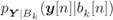
If instead of information-theoretic considerations, we want to analyze the performance of a decoder in terms of decoding error probability, we may use the analysis and tools described in Section 6.2.4. The word-error probability (WEP) can be then approximated as
where
![]() , and
, and ![]() are the corrected L-values corresponding to the
are the corrected L-values corresponding to the ![]() nonzero bits in the error codeword
nonzero bits in the error codeword ![]() .
.
Here, as in Section 6.2.4, we consider only the error codewords ![]() whose nonzero bits are mapped to different time instants
whose nonzero bits are mapped to different time instants ![]() . This assumption (already discussed in Section 6.2.4) allows us to treat all the L-values
. This assumption (already discussed in Section 6.2.4) allows us to treat all the L-values ![]() as independent.
as independent.
The condition (ii) in Definition 7.11 is useful again to ensure uniqueness of the solutions, as we note that multiplication of all the L-values by a common factor ![]() does not change the PEP.
does not change the PEP.
The PEP-optimal correction indeed minimizes the PEP independently of the GHW ![]() . This is a consequence of the assumption of the L-values being independent. Moreover, we note that the PEP-optimal and GMI-optimal correction functions are the same.
. This is a consequence of the assumption of the L-values being independent. Moreover, we note that the PEP-optimal and GMI-optimal correction functions are the same.
7.3 Suboptimal Correction of L-values
In Section 7.2, we defined the optimal correction function ![]() . However, as finding or implementing
. However, as finding or implementing ![]() is not necessarily simple, we use it as a reference rather than as a practical approach. Moreover, its form may provide us with guidelines to design suboptimal but simple-to-implement correction functions. This is the objective of this section.
is not necessarily simple, we use it as a reference rather than as a practical approach. Moreover, its form may provide us with guidelines to design suboptimal but simple-to-implement correction functions. This is the objective of this section.
Our objective is to find a suitable approximate correction function
where ![]() represents parameters of the approximate correction function. Because of the approximation in (7.43), the corrected L-values are still mismatched, i.e., we lose the relationship with their interpretation in terms of a posteriori probabilities or likelihoods.
represents parameters of the approximate correction function. Because of the approximation in (7.43), the corrected L-values are still mismatched, i.e., we lose the relationship with their interpretation in terms of a posteriori probabilities or likelihoods.
7.3.1 Adaptation Strategies
To find a correction function ![]() , first we need to decide on the form of the approximate function, and then, we have to find the parameters
, first we need to decide on the form of the approximate function, and then, we have to find the parameters ![]() . There are essentially two different ways to “adapt” the correction parameters
. There are essentially two different ways to “adapt” the correction parameters ![]() , which we present schematically in Fig. 7.3:
, which we present schematically in Fig. 7.3:
- Feedback-Based Adaptation consists in adjusting the correction parameters using the decoding results. Such an approach requires off-line simulations in the targeted conditions of operation. The advantage is that we explicitly optimize the criterion of interest (e.g., bit-error probability (BEP) after decoding). The disadvantage, however, is that, in most cases, we need to carry out an exhaustive search over the entire domain of the correction parameters. While this is acceptable if only a few parameters need to be found, it is unfeasible when the number of parameters is large or when the operating conditions (such as the SNR or the interference level) are variable.
- Predictive Adaptation consists in finding the parameters of the correction function from the PDF of the mismatched L-values and from the model of the decoder. The postulate, inspired by the optimal correction in Section 7.2, is that the correction should be done for each of the mismatched L-values independently of the others. The caveat is that a simple strategy to deal with the mismatch needs to be devised.

Figure 7.3 Finding the parameters  of the correction function via (a) a feedback-based strategy where the parameters are adjusted using the statistics of the output (e.g., the decoding results), and (b) a predictive strategy where the parameters are adjusted, before decoding, using the PDF of the mismatched L-values only
While the feedback-based adaptation is robust and may be interesting to use from a practical point of view, it has little theoretical interest and provides no insights into the correction principles. In this chapter, we focus on predictive adaptation strategies.
Probably the simplest correction is done via a linear function
which has an appealing simplicity. Furthermore, in many cases, ![]() is observed to be relatively “well” approximated by a linear function, see, e.g., Example 7.10.
is observed to be relatively “well” approximated by a linear function, see, e.g., Example 7.10.
In the following, we will discuss different ways of determining the optimal values of ![]() . The first one is based on a heuristic approach based on function fitting, the second one aims at maximizing achievable rates of the resulting mismatched decoder, and the third one aims at minimizing the decoding error probability. It is important to note that the maximization of achievable rates and the minimization of the error probability are not the same for the (suboptimal) linear correction we consider here.
. The first one is based on a heuristic approach based on function fitting, the second one aims at maximizing achievable rates of the resulting mismatched decoder, and the third one aims at minimizing the decoding error probability. It is important to note that the maximization of achievable rates and the minimization of the error probability are not the same for the (suboptimal) linear correction we consider here.
7.3.2 Function Fitting
A heuristic adaptation strategy aiming at fulfilling the condition (7.43) is based on finding the parameter ![]() which approximates “well”
which approximates “well” ![]() (which is PEP- and GMI-optimal). As an example, we consider here the weighted least-squares fit (WLSF)
(which is PEP- and GMI-optimal). As an example, we consider here the weighted least-squares fit (WLSF)
where the fitting criterion is defined as
The expectation in (7.46) is meant to provide a strong fit between the two functions for the cases which are most likely to be observed, i.e., the squared fitting-error is weighted by the PDF of the L-values.
The WLSF approach has two main drawbacks:
- The objective function (7.45) is not directly related to the performance of the decoder, so there is no guarantee that the correction will improve its performance. While (7.45) can be changed, devising the appropriate criterion remains a challenge.
- The function
 is explicitly used in the optimization, so the form of the PDF
  has to be known, cf. (7.29). This points out to a practical difficulty: while we might obtain the form of the PDF if we knew how the mismatched L-values were calculated (e.g., via the techniques shown in Chapter 5), this approach may be too complicated or impossible, e.g., when the mismatch is caused by modeling errors. Then we have to use histograms to estimate
  , which requires extensive simulations.
Before proceeding further, we introduce a lemma that we will use in the following subsections.
7.3.3 GMI-Optimal Linear Correction
The GMI-optimality principle in Section 7.2 has to be revisited taking into account the fact that we constrain the correction function to have a linear form. To this end, we rewrite (7.23) as
where, for notation simplicity, in (7.51) we use ![]() , and
, and ![]() is the solution of the optimization problem in the right-hand side (r.h.s.) of (7.51). Owing to Theorem 4.22, this solution is known to be unique.
is the solution of the optimization problem in the right-hand side (r.h.s.) of (7.51). Owing to Theorem 4.22, this solution is known to be unique.
To analyze the effect of the linear correction of the L-values ![]() on the GMI, we move the correction effect from the L-values' domain to the domain of the metrics
on the GMI, we move the correction effect from the L-values' domain to the domain of the metrics ![]() . From (7.16), we obtain the relationship between the corrected and the uncorrected metrics, i.e.,
. From (7.16), we obtain the relationship between the corrected and the uncorrected metrics, i.e.,

By comparing (7.16) with (7.55), we conclude that the linear correction implies that the corrected decoding metric depends on the “neutral” metric via
Which, when used in (7.21) yields
Therefore, in order to maximize the GMI in (7.52) using linear correction functions, we have to solve the following optimization problem:
where ![]() . The solution to the problem in (7.58) is given in the following theorem.
. The solution to the problem in (7.58) is given in the following theorem.
It is important to note that the correction via ![]() does not change the maximum value of the bitwise GMI, i.e.,
does not change the maximum value of the bitwise GMI, i.e.,
Instead, the objective of the correction is to “align” the maxima for each ![]() , i.e., to make them occur for the same value of
, i.e., to make them occur for the same value of ![]() , and thus, maximize the sum.
, and thus, maximize the sum.

Figure 7.4 Linear correction of the L-values in the presence of an SNR mismatch. Thanks to the correction of the L-values  by the optimal factors
  in (7.62), the maxima of all the functions
  are aligned at
  , and their sum is then maximized. In this example,
  so
so  , and thus, the bitwise GMI functions before and after correction are the same. The gain offered by the correction in terms of GMI is also shown
7.3.4 PEP-Optimal Linear Correction
Considering the linear correction, (7.37) becomes
and the PEP is given by
where the PDF of the random variable ![]() is given by
is given by
where (7.66) follows from (7.63).
In order to minimize the upper bound on the performance of the decoder in (7.35), we should find ![]() that minimizes
that minimizes ![]() for all
for all ![]() , i.e.,
, i.e.,
At first sight, the PEP minimization problem in (7.67) may appear intractable because of the dependence on the unknown ![]() affecting the convolution of the PDFs in (7.65). It is thus instructive to have a look at a very simple case which we show in the following example.
affecting the convolution of the PDFs in (7.65). It is thus instructive to have a look at a very simple case which we show in the following example.
The results in Example 7.16 show that the correction factor in this case is independent of ![]() . While this is an encouraging conclusion, recall that we solved the PEP-minimization problem (7.67), thanks to the Gaussian form of the PDF. As we cannot do this for arbitrary distributions, we now turn our attention to approximations.
. While this is an encouraging conclusion, recall that we solved the PEP-minimization problem (7.67), thanks to the Gaussian form of the PDF. As we cannot do this for arbitrary distributions, we now turn our attention to approximations.
Consider the upper (Chernoff) bound we introduced in Theorem 6.29 and generalized to the case of nonidentically distributed L-values in (6.355). We upper bound (7.64) as
where ![]() is the cumulant-generating function (CGF) of the corrected L-value
is the cumulant-generating function (CGF) of the corrected L-value ![]() conditioned on
conditioned on ![]() .
.
It may be argued that the upper bound on the PEP may not be tight and more accurate approximations or even the exact numerical expressions we discussed in Section 6.3.3 should be used. While this might be done, more involved expressions would not allow us to find simple (and independent of ![]() ) analytical rules for correction. Moreover, the numerical examples (see, e.g., Example 6.30) indicate that the upper bound follows the actual value of the PEP very closely (up to a multiplicative factor), so more involved expressions are unlikely to offer significant gains.
) analytical rules for correction. Moreover, the numerical examples (see, e.g., Example 6.30) indicate that the upper bound follows the actual value of the PEP very closely (up to a multiplicative factor), so more involved expressions are unlikely to offer significant gains.
With this cautionary statement, we will refer to the rule defined in Theorem 7.76 as the PEP-optimal linear correction.
7.3.5 GMI- and PEP-Optimal Linear Corrections: A Comparison
To gain a quick insight into the differences between the GMI- and PEP-optimal corrections based on linear correction strategies, in what follows, we rewrite the optimality conditions in both cases, assuming the bits are uniformly distributed (i.e., ![]() ) and the symmetry condition (3.74) is satisfied.
) and the symmetry condition (3.74) is satisfied.
As the GMI is concave on ![]() (see Theorem 4.22), a necessary and sufficient condition for the maximization of the bitwise GMI is given by
(see Theorem 4.22), a necessary and sufficient condition for the maximization of the bitwise GMI is given by
Using Theorem 7.3 and (4.94), we then obtain a condition which has to be satisfied by the GMI-optimal correction factor ![]()
where, to pass from (7.82) to (7.83), we used ![]() .
.
Similarly, the PEP-minimization condition in (7.76) states that the saddlepoint should be related to the correction factor via ![]() , which may be written as follows:
, which may be written as follows:
which implies
Comparing (7.83) and (7.85) we see that, in general, GMI-optimal and PEP-optimal linear correction factors will not be the same. This may come as a surprise because we know from Section 7.2 that the GMI-optimal and PEP-optimal correction functions are the same. Here, however, we are restricting our analysis to linear correction functions, while the optimal function are nonlinear in general. This constraint produces different results.
As for the practical aspects of using both correction principles, the main difference lies in the complexity of the search for the optimal scaling factor. In most cases, finding the maximum GMI will require numerical quadratures as the nonlinear functions will resist analytical integration, e.g., the hyperbolic cosine in (7.83). On the other hand, the PEP-optimal correction relies on the knowledge of the moment-generating function (MGF) of the PDF of the L-values, which, in some cases, may be calculated analytically. Consequently, finding the correction factor will be simplified, as we will illustrate in Section 7.3.6.
In both cases, if ![]() is not known, Monte Carlo integration may be used to calculate the integrals (7.83) or (7.85), cf. (6.311) and (4.89), and then, the complexity of adaptation is similar for both approaches.
is not known, Monte Carlo integration may be used to calculate the integrals (7.83) or (7.85), cf. (6.311) and (4.89), and then, the complexity of adaptation is similar for both approaches.
7.3.6 Case Study: Correcting Interference Effects
To illustrate the previous findings, we consider transmission using a 2PAM constellation, where the transmitted symbols ![]() pass through a channel corrupted with additive white Gaussian noise (AWGN) and a 2PAM-modulated interference, i.e.,
pass through a channel corrupted with additive white Gaussian noise (AWGN) and a 2PAM-modulated interference, i.e.,
where ![]() is the channel gain,
is the channel gain, ![]() is Gaussian noise with variance
is Gaussian noise with variance ![]() , and
, and ![]() is the interference signal received with gain
is the interference signal received with gain ![]() . We assume that the channel gains
. We assume that the channel gains ![]() and
and ![]() are known (estimated) and
are known (estimated) and ![]() , i.e., the interference is weaker than the desired signal.
, i.e., the interference is weaker than the desired signal.
The instantaneous SNR is defined as ![]() , the instantaneous signal-to-interference ratio (SIR) as
, the instantaneous signal-to-interference ratio (SIR) as ![]() , and the average SIR is given by
, and the average SIR is given by ![]() . We assume that the channel is memoryless, and thus, the time index
. We assume that the channel is memoryless, and thus, the time index ![]() is dropped. The model (7.86) may be written using random variables as
is dropped. The model (7.86) may be written using random variables as
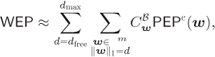
From (7.2), it is simple to calculate exactly the L-values in this case as
where
We assume now that the receiver ignores the presence of the interference (which is equivalent to using ![]() in (7.89)). The L-values are obtained as in (3.65), i.e.,
in (7.89)). The L-values are obtained as in (3.65), i.e.,
and are—because of the assumed absence of interference—mismatched.
To find the correction factors in the case of the PEP-optimal correction, we need to calculate the CGF of ![]() , conditioned on a transmitted bit
, conditioned on a transmitted bit ![]() , or, equivalently, on
, or, equivalently, on ![]() . As
. As ![]() is a sum of independent random variables
is a sum of independent random variables ![]() , and
, and ![]() , we obtain its CGF as follows:
, we obtain its CGF as follows:
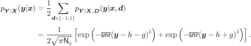
Setting the derivative of (7.94) with respect to ![]() to zero and using
to zero and using ![]() , we obtain the nonlinear equation
, we obtain the nonlinear equation
solved by ![]() , which we interpret graphically in Fig. 7.5 as the intersection of the r.h.s. and l.h.s. of (7.95).
, which we interpret graphically in Fig. 7.5 as the intersection of the r.h.s. and l.h.s. of (7.95).

Figure 7.5 Solving the saddlepoint equation (7.95) graphically for (a) low SNR, where  , and (b) high SNR, where
  . The solution of (7.95) is shown as a large circle and the solutions corresponding to the approximations
  and
and  as squares
In general, we may solve (7.95) numerically; however, using approximations, closed-form approximations may be obtained in particular cases, Namely, for ![]() , using the linearization
, using the linearization ![]() (shown as a dashed line in Fig. 7.5) in (7.95), we obtain
(shown as a dashed line in Fig. 7.5) in (7.95), we obtain
and then for a given ![]() , we see that
, we see that
The corrected L-values are next calculated as
which is similar to (7.90) but with the denominator now having the meaning of the noise and interference power. This means that the effect of the noise and the interference is modeled as a Gaussian random variable with variance ![]() . Such a model is, indeed, appropriate for low SNR, when the noise “dominates” the interference. We also note that, using
. Such a model is, indeed, appropriate for low SNR, when the noise “dominates” the interference. We also note that, using
and
in (7.31), yields exactly the same results ![]() .
.
We note that we always have ![]() (see Fig. 7.5), i.e., we have to scale down the L-values to decrease their reliability (expressed by their amplitude); in other words, they are too “optimistic” when calculated ignoring the interference. On the other hand, as
(see Fig. 7.5), i.e., we have to scale down the L-values to decrease their reliability (expressed by their amplitude); in other words, they are too “optimistic” when calculated ignoring the interference. On the other hand, as ![]() , we conclude that assuming a Gaussian interference is too pessimistic.
, we conclude that assuming a Gaussian interference is too pessimistic.
For high SNR (i.e., when ![]() ) we take advantage of the “saturation” approximation
) we take advantage of the “saturation” approximation ![]() , which used in (7.7) yields the correction factor
, which used in (7.7) yields the correction factor
The corrected L-values in this case are calculated as
which is, again, similar to (7.90), but now the gain of the desired signal ![]() is reduced by the interference-related term
is reduced by the interference-related term ![]() . This can be explained as follows: for high SNR, the interference can be “distinguished” from the noise and becomes part of the transmitted constellation, i.e., by sending bit
. This can be explained as follows: for high SNR, the interference can be “distinguished” from the noise and becomes part of the transmitted constellation, i.e., by sending bit ![]() , we will effectively be able to differentiate between
, we will effectively be able to differentiate between ![]() and
and ![]() . Moreover, for high SNR, the symbol that is the most likely to provoke the error is the one closest to the origin, i.e.,
. Moreover, for high SNR, the symbol that is the most likely to provoke the error is the one closest to the origin, i.e., ![]() . This leads to assuming that 2PAM symbols are sent over a channel with gain
. This leads to assuming that 2PAM symbols are sent over a channel with gain ![]() .
.
To obtain the GMI-optimal factor ![]() we numerically solve (7.82)
we numerically solve (7.82)
using
with ![]() given by (7.89).
given by (7.89).
In Fig. 7.6, we show the values of the optimal correction factors as a function of SNR for different values SIR, where we can appreciate that GMI-optimal correction factors ![]() in (7.59) are not identical but close to
in (7.59) are not identical but close to ![]() . Both factors increase with SIR, as the case
. Both factors increase with SIR, as the case ![]() corresponds to the assumed absence of interference, i.e.,
corresponds to the assumed absence of interference, i.e., ![]() . For comparison, in this figure, we also show the results of the ad hoc WLSF correction defined in (7.45) and (7.46). We can expect it to provide adequate results when
. For comparison, in this figure, we also show the results of the ad hoc WLSF correction defined in (7.45) and (7.46). We can expect it to provide adequate results when ![]() is almost linear, i.e., when the PDF
is almost linear, i.e., when the PDF ![]() is close to the Gaussian form (see Corollary 7.8). This happens when theinterference is dominated by the noise, i.e., for low SNR and high SIR and then, as we can see in Fig. 7.6,
is close to the Gaussian form (see Corollary 7.8). This happens when theinterference is dominated by the noise, i.e., for low SNR and high SIR and then, as we can see in Fig. 7.6, ![]() is close to the GMI- and PEP-optimal correction. The results obtained are very different when the SNR increases.
is close to the GMI- and PEP-optimal correction. The results obtained are very different when the SNR increases.

Figure 7.6 Linear correction factors  solving (7.103),
  solving (7.95), and
  in (7.45) as a function of SNR for various values of SIR. We may appreciate that for low SNR, the correction factors tend to
  (see (7.97)), and for high SNR, they tend to
  (see (7.101))
To verify how the correction affects the performance of a practical decoder, we consider a block of ![]() bits encoded using a convolutional encoder (CENC) with rate
bits encoded using a convolutional encoder (CENC) with rate ![]() and generating polynomials
and generating polynomials ![]() (see Table 2.1) as well as by the turbo encoder (TENC) with rate
(see Table 2.1) as well as by the turbo encoder (TENC) with rate ![]() from Example 2.31. We assume that
from Example 2.31. We assume that ![]() and
and ![]() are Rayleigh random variables with
are Rayleigh random variables with ![]() and
and ![]() . The average SNR is
. The average SNR is ![]() . Thus, we may observe the effect of interference level by changing the value of
. Thus, we may observe the effect of interference level by changing the value of ![]() . The correction factor has to be found for each value of
. The correction factor has to be found for each value of ![]() and
and ![]() , which we assumed were perfectly known at the receiver. The fact that we know the interference gain
, which we assumed were perfectly known at the receiver. The fact that we know the interference gain ![]() but we do not use it in (7.89) allows us to highlight the functioning of the correction principle and shows the eventual gain of more complex processing in (7.89).
but we do not use it in (7.89) allows us to highlight the functioning of the correction principle and shows the eventual gain of more complex processing in (7.89).
The average SIR is set to ![]() for the CENC and
for the CENC and ![]() for the TENC. The results of the decoding in terms of BEP are shown in Fig. 7.7. For the CENC we used a maximum likelihood (ML) (Viterbi) decoder and for the TENC a turbo decoder with five iterations. Figure 7.7 shows the BEP for different correction strategies, where, for comparison, we also show the results of the decoding using exact L-values obtained via (7.88).
for the TENC. The results of the decoding in terms of BEP are shown in Fig. 7.7. For the CENC we used a maximum likelihood (ML) (Viterbi) decoder and for the TENC a turbo decoder with five iterations. Figure 7.7 shows the BEP for different correction strategies, where, for comparison, we also show the results of the decoding using exact L-values obtained via (7.88).
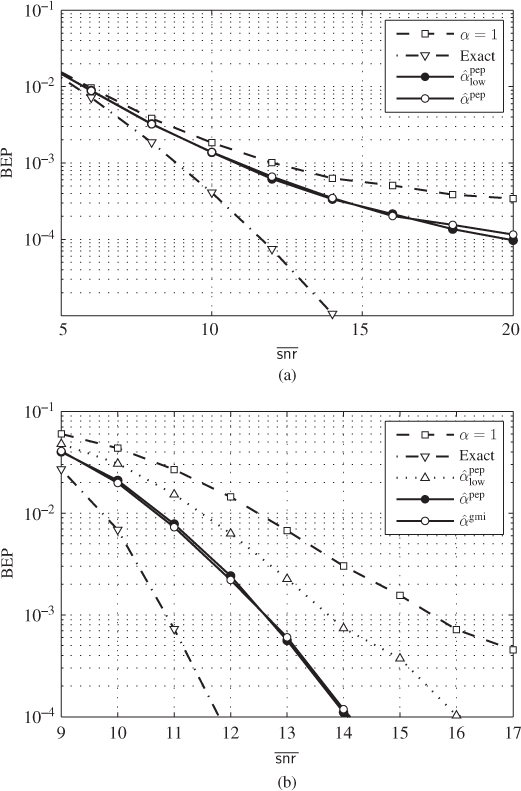
Figure 7.7 BEP results for (a) a CENC with  and (b) a TENC with
  obtained using L-values without correction (7.90) (
 ), L-values with PEP-optimal correction (calculated solving (7.95)), exact L-values (7.88), and L-values corrected using
  . For the TENC, the results obtained using a Gaussian model for the L-values are also shown (
 )
)
The results in Fig. 7.7 show that the correction results based on the PEP- and the GMI-optimal approaches are similar and manage to partially bridge the gap to the results based on exact L-values. The performance improvement is particularly notable for high average SNR, which is consistent with the results of Fig. 7.6, where the most notable correction (small values of ![]() ) are also obtained for high SNR.
) are also obtained for high SNR.
In Fig. 7.7, we also show the results of the correction derived assuming that the interference is Gaussian, yielding the correction factor ![]() . This coefficient is independent of the channel gains
. This coefficient is independent of the channel gains ![]() , and thus, common to all the L-values and irrelevant to the performance of an ML decoder. For this reason, the results obtained with
, and thus, common to all the L-values and irrelevant to the performance of an ML decoder. For this reason, the results obtained with ![]() and with
and with ![]() are identical for the CENC, where the ML (Viterbi) decoder is used, and thus, not shown in Fig. 7.7 (a). On the other hand, the turbo decoder, based on the iterative exchange of information between the constituent decoders, depends on an accurate representation of the a posteriori probabilities via the L-values. It is, therefore, sensitive to the scaling, which is why the correction with
are identical for the CENC, where the ML (Viterbi) decoder is used, and thus, not shown in Fig. 7.7 (a). On the other hand, the turbo decoder, based on the iterative exchange of information between the constituent decoders, depends on an accurate representation of the a posteriori probabilities via the L-values. It is, therefore, sensitive to the scaling, which is why the correction with ![]() improves the decoding results.
improves the decoding results.
As might be expected from the results shown in Fig. 7.6, the BEP results do not change significantly when using GMI- or PEP-optimal linear correction. However, this example also clearly demonstrates that the PEP provides a much simpler approach to find the correction factor, which we obtained analytically, thanks to the adopted approximations.
7.4 Bibliographical Notes
Dealing with incorrectly evaluated or mismatched likelihoods can be traced back to early works in the context of iterative decoders, where simplified operations in one iteration affect the performance of the subsequent ones. This has been observed in the context of the decoding of turbo codes (TCs) [1–6] or low-density parity-check (LDPC) codes [7 8]. The problem of mismatched L-values in the demapper, which was the focus of this chapter, was analyzed in [9–12]. The main difference between the analysis of the decoder and the demapper is that, in the latter, we may characterize analytically the distribution of the L-values. When the L-values follow a Gaussian distribution, a linear correction is optimal. As the Gaussian model is simple to deal with, the linear correction was very often assumed. This was also motivated by the simplicity of the resulting implementation and the simplified search of the scalar correction parameter [1–3]. This linear scaling, in fact, evolved as a heuristic compensation, and was studied in various scenarios [4 13–16]. Multiparameter correction functions have also been studied, e.g., in [17 18].
The feedback-based adaptation approach can be applied in the absence of simple models relating the parameters of the L-values to the decoding outcome (e.g., BEP).This is necessary when the results are obtained via actual implementation of the decoding algorithm on many different realizations of the channel outcome [2 3], or when they are predicted using semi-analytical tools such density evolution (in the case of LDPC codes [17]) or extrinsic transfer charts (in the case of TCs [8]). In such cases, the correction factor is found through a brute-force search over the entire space of parameters, i.e., among the results obtained for different correction factors, the one ensuring the best performance is deemed optimal [2 3, 6 7, 19]. While this is a pragmatic approach when searching for one [7] or two [18] correction factors, it becomes very tedious when many [17] correction factors have to be found, because of the increased dimensionality of the search space.
The formalism of the decoding based on the mismatched metrics (the mismatched decoding perspective for BICM) was introduced in [20]. The idea of the optimal correction function from Section 7.2 was shown in [3] and formally developed as GMI-optimal in [21]. This inspired the idea of the GMI-optimal linear correction via the so-called “harmonization” of the GMI curves introduced in [10] and described in Section 7.3.3. Examples of applications can be found in [10–12 22]. The PEP-optimal linear correction we presented in Section 7.3.4 was introduced in [12].
As explained in Section 7.3, the predictive adaptation approach exploits the knowledge of the probabilistic model of the L-values. Some works focused on ensuring that the corrected L-values are consistent [8 23, 24]. This was achieved by using a heuristically adopted criterion, e.g., (7.45), and by estimating the PDF via histograms. As this approach is quite tedious, parameterization of the PDF may be used. In particular, a Gaussian model was used in [1] and a Gaussian mixture model in [18]. The drawback of these approaches is that the PDF must be estimated. More importantly, a good fit between the linear form and the optimal function does not necessarily translate into the decoding gains. On the other hand, the GMI-optimal and PEP-optimal methods formally address the problem of improving the performance of the decoder. These predictive approaches optimize the GMI and minimize the CGF, respectively. In the cases where we do not know the PDF, both the GMI and the CGF can be found via Monte Carlo simulations, which is still simpler than estimating the PDF itself.
References
- [1] Papke, L., Robertson, P., and Villebrun, E. (1996) Improved decoding with the SOVA in a parallel concatenated (turbo-code) scheme. IEEE International Conference on Communications (ICC), June 1996, Dallas, TX.
- [2] Vogt, J. and Finger, A. (2000) Improving the max-log-map turbo decoder. IEEE Electron. Lett., 36 (23), 1937–1939.
- [3] van Dijk, M., Janssen, A., and Koppelaar, A. (2003) Correcting systematic mismatches in computed log-likelihood ratios. Eur. Trans. Telecommun., 14 (3), 227–224.
- [4] Ould-Cheikh-Mouhamedou, Y., Guinand, P., and Kabal, P. (2003) Enhanced Max-Log-APP and enhanced Log-APP decoding for DVB-RCS. International Symposium on Turbo Codes and Related Topics, May 2003, Brest, France.
- [5] Huang, C. X. and Ghrayeb, A. (2006) A simple remedy for the exaggerated extrinsic information produced by the SOVA algorithm. IEEE Trans. Wireless Commun., 5 (5), 996–1002.
- [6] Alvarado, A., Núñez, V., Szczecinski, L., and Agrell, E. (2009) Correcting suboptimal metrics in iterative decoders. IEEE International Conference on Communications (ICC), June 2009, Dresden, Germany.
- [7] Chen, J. and Fossorier, M. (2002) Near optimum universal belief propagation based decoding of low-density parity check codes. IEEE Trans. Commun., 50 (3), 406–414.
- [8] Lechner, G. (2007) Efficient decoding techniques for LDPC codes. PhD dissertation, Vienna University of Technology, Vienna, Austria.
- [9] Classon, B., Blankenship, K., and Desai, V. (2002) Channel coding for 4G systems with adaptive modulation and coding. IEEE Wireless Commun. Mag., 9 (2), 8–13.
- [10] Nguyen, T. and Lampe, L. (2011) Bit-interleaved coded modulation with mismatched decoding metrics. IEEE Trans. Commun., 59 (2), 437–447.
- [11] Yazdani, R. and Ardakani, M. (2011) Efficient LLR calculation for non-binary modulations over fading channels. IEEE Trans. Commun., 59 (5), 1236–1241.
- [12] Szczecinski, L. (2012) Correction of mismatched L-values in BICM receivers. IEEE Trans. Commun., 60 (11), 3198–3208.
- [13] Pyndiah, R. M. (1998) Near-optimum decoding of product codes: block turbo codes. IEEE Trans. Commun., 46 (8), 1003–1010.
- [14] Crozier, S., Gracie, K., and Hunt, A. (1999) Efficient turbo decoding techniques. 11th International Conference on Wireless Communications, July 1999, Calgary, AB, Canada.
- [15] Gracie, K., Crozier, S., and Guinand, P. (2004) Performance of an mlse-based early stopping technique for turbo codes. IEEE Vehicular Technology Conference (VTC-Fall), Los Angeles, CA.
- [16] Gracie, K., Hunt, A., and Crozier, S. (2006) Performance of turbo codes using MLSE-based early stopping and path ambiguity checking for input quatized to 4 bits. International Symposium on Turbo Codes and Related Topics, April 2006, Munich, Germany.
- [17] Zhang, J., Fossorier, M., Gu, D., and Zhang, J. (2006) Two-dimensional correction for Min-Sum decoding of irregular LDPC codes. IEEE Commun. Lett., 10 (3), 180–182.
- [18] Jia, Q., Kim, Y., Seol, C., and Cheun, K. (2009) Improving the performance of SM-MIMO/BICM-ID systems with LLR distribution matching. IEEE Trans. Commun., 57 (11), 3239–3243.
- [19] Heo, J. and Chugg, K. (2005) Optimization of scaling soft information in iterative decoding via density evolution methods. IEEE Trans. Commun., 53 (6), 957–961.
- [20] Martinez, A., Guillén i Fàbregas, A., Caire, G., and Willems, F. M. J. (2009) Bit-interleaved coded modulation revisited: a mismatched decoding perspective. IEEE Trans. Inf. Theory, 55 (6), 2756–2765.
- [21] Jaldén, J., Fertl, P., and Matz, G. (2010) On the generalized mutual information of BICM systems with approximate demodulation. IEEE Information Theory Workshop (ITW), January 2010, Cairo, Egypt.
- [22] Nguyen, T. and Lampe, L. (2011) Mismatched bit-interleaved coded noncoherent orthogonal modulation. IEEE Commun. Lett., 15 (5), 563–565.
- [23] Lechner, G. and Sayir, J. (2004) Improved sum-min decoding of LDPC codes. International Symposium on Information Theory and its Applications (ISITIA), October 2004, Parma, Italy.
- [24] Lechner, G. and Sayir, J. (2006) Improved sum-min decoding for irregular LDPC codes. International Symposium on Turbo Codes and Related Topics, April 2006, Munich, Germany.