
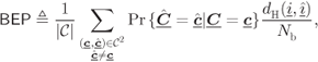
6.1.3 Bounding Techniques
The approach we used to evaluate the TP in 2D constellations can be extended to the general ![]() -dimensional case. However, the geometric considerations get more tedious as the dimension of the integration space increases. Therefore, simple approximations are often used, which may also be sufficient for the purpose of the analysis and/or design. A popular approach relies on finding an upper bound on the TP
-dimensional case. However, the geometric considerations get more tedious as the dimension of the integration space increases. Therefore, simple approximations are often used, which may also be sufficient for the purpose of the analysis and/or design. A popular approach relies on finding an upper bound on the TP ![]() , which we do in the following.
, which we do in the following.
For a given ![]() , and for any
, and for any ![]() with
with ![]() , we have
, we have
which follows from the fact that, by using one inequality, we relax the constraint imposed by ![]() inequalities defining
inequalities defining ![]() . The TP is therefore upper bounded, for any
. The TP is therefore upper bounded, for any ![]() , as
, as
Setting ![]() we obtain the bound
we obtain the bound
where
It is easy to see that
is the PEP, i.e., the probability that after transmitting ![]() , the likelihood
, the likelihood ![]() is larger than the likelihood
is larger than the likelihood ![]() (or equivalently, that the received signal
(or equivalently, that the received signal ![]() is closer to
is closer to ![]() than to
than to ![]() ). We can calculate (6.75) as
). We can calculate (6.75) as
To tighten the bound in (6.74), we note that (6.73) is true for any ![]() , so a better bound is obtained via
, so a better bound is obtained via
where
with
In other words, we find the index ![]() of the linear form
of the linear form ![]() defining the Voronoi region
defining the Voronoi region ![]() such that
such that ![]() , so as to maximize the distance between the half-space
, so as to maximize the distance between the half-space ![]() and
and ![]() , and next, we calculate the probability that, conditioned on
, and next, we calculate the probability that, conditioned on ![]() , the observation
, the observation ![]() falls into the half-space we found, i.e., that the 1D projection of the zero-mean Gaussian random variable
falls into the half-space we found, i.e., that the 1D projection of the zero-mean Gaussian random variable ![]() falls in the interval
falls in the interval ![]() .
.
To tighten the bound even further, instead of finding the half-space that contains ![]() , we can consider finding the wedge containing
, we can consider finding the wedge containing ![]() , i.e., we generalize the bound in (6.80) as
, i.e., we generalize the bound in (6.80) as
where

where ![]() and
and ![]() are the indices minimizing (6.85).5
are the indices minimizing (6.85).5
It is easy to see that the three bounds presented above satisfy
Among the three bounds, the PEP-based bound in (6.74) is the simplest one. Not surprisingly, however, with decreasing implementation complexity, the accuracy of the approximation also decreases. On the other hand, the two bounds in (6.81) and (6.85) are tighter, but algorithmic, i.e., they require optimizations to find the relevant linear forms. The advantage of (6.81) and (6.85) is that they can be used for any ![]() -dimensional constellation, but at the same time, they are based on 1D or 2D integrals (and not on
-dimensional constellation, but at the same time, they are based on 1D or 2D integrals (and not on ![]() -dimensional ones).
-dimensional ones).

Figure 6.9 Evaluation of TPs for 8PSK and the AWGN channel: (a)  , (b)
, (b)  , (c)
, (c)  , and (d)
6.1.4 Fading Channels
The previous analysis is valid for the case of nonfading channel, i.e., for transmission with fixed SNR. Although we did not make it explicit in the notation, the BEP depends on the SNR, i.e., ![]() . The BEP for fading channels should then be calculated averaging the previously obtained expressions over the distribution of the SNR, i.e.,
. The BEP for fading channels should then be calculated averaging the previously obtained expressions over the distribution of the SNR, i.e.,

where
In the previous sections we have shown that the TP ![]() can always be expressed via Q-functions
can always be expressed via Q-functions ![]() or via bivariate Q-functions
or via bivariate Q-functions ![]() . But because
. But because ![]() , to obtain (6.98) it is enough to find
, to obtain (6.98) it is enough to find ![]() . In order to calculate the latter we will exploit the following alternative form of the bivariate Q-function (2.11) valid for any
. In order to calculate the latter we will exploit the following alternative form of the bivariate Q-function (2.11) valid for any ![]()

where

and
The expression in (6.99) can be used for any ![]() ; however, some of the expressions we developed for the TP have negative arguments. For these cases, we use the identity
; however, some of the expressions we developed for the TP have negative arguments. For these cases, we use the identity

The results in (6.102) show that to evaluate (6.98), it is enough to consider the case ![]() . The following theorem gives a general expression for the expectation
. The following theorem gives a general expression for the expectation ![]() for Nakagami-
for Nakagami-![]() fading channels.
fading channels.
The main challenge now consists in calculating ![]() . In what follows we provide a closed-form expression without giving a proof. Such a proof can be found in the references we cite in Section 6.5. The closed-form expression for
. In what follows we provide a closed-form expression without giving a proof. Such a proof can be found in the references we cite in Section 6.5. The closed-form expression for ![]() and any
and any ![]() is
is

where
![]() for
for ![]() and
and ![]() .
.

Figure 6.10 Evaluation of TPs for 8PSK in Rayleigh fading channel

Figure 6.11 BEP  and the corresponding bounds
  for
for  and an 8PSK constellation labeled by the BRGC in a Rayleigh fading channel
6.2 Coded Transmission
When trying to analyze the performance of the decoder we face issues similar to those appearing in the uncoded case. However, because geometric considerations would require high-dimensional analysis, exact solutions are very difficult to find. Instead, we resort to bounding techniques based on the evaluation of PEPs, which are similar in spirit to those presented in Section 6.1.3.
The decisions made by the maximum likelihood (ML) and the BICM decoders can both be expressed as (see (3.9) and (3.22))
where ![]() is a decoding metric that depends on the considered decoder. Note that with a slight abuse of notation, throughout this chapter we also use the notation
is a decoding metric that depends on the considered decoder. Note that with a slight abuse of notation, throughout this chapter we also use the notation ![]() and
and ![]() to denote this metric.
to denote this metric.
An error occurs when the decoded codeword ![]() is different from the transmitted one
is different from the transmitted one ![]() . The probability of detecting an incorrect codeword is the so-called WEP and is defined as
. The probability of detecting an incorrect codeword is the so-called WEP and is defined as
where ![]() and
and ![]() are the random variables representing, respectively, the transmitted and detected codewords.
are the random variables representing, respectively, the transmitted and detected codewords.
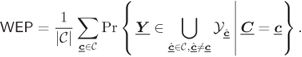
The WEP can be expressed as

where ![]() denotes the pairs
denotes the pairs ![]() taken from
taken from ![]() and to obtain (6.132) we assumed equiprobable codewords, i.e.,
and to obtain (6.132) we assumed equiprobable codewords, i.e., ![]() .
.
Similarly, weighting the error events by the relative number of information bits in error, we obtain the average BEP, defined as
where ![]() and
and ![]() are the sequences of information bits corresponding to the codewords
are the sequences of information bits corresponding to the codewords ![]() and
and ![]() , respectively.
, respectively.
6.2.1 PEP-Based Bounds
The expressions (6.132) and (6.133) show that the main issue in evaluating the decoder's performance boils down to an efficient calculation of
where ![]() is the decision region of the codeword
is the decision region of the codeword ![]() defined as
defined as
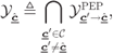
where
As in the case of uncoded transmission, the evaluation of ![]() in (6.134) boils down to finding the decision region
in (6.134) boils down to finding the decision region ![]() and, more importantly, to evaluating the multidimensional integral in (6.135). Since usually
and, more importantly, to evaluating the multidimensional integral in (6.135). Since usually ![]() is very large, the exact calculation of this
is very large, the exact calculation of this ![]() -dimensional integral is most often considered infeasible. One of the most popular simplifications to tackle this problem is based on a PEP-based bounding technique. Let the PEP be defined as
-dimensional integral is most often considered infeasible. One of the most popular simplifications to tackle this problem is based on a PEP-based bounding technique. Let the PEP be defined as
By knowing that ![]() and using
and using ![]() we can then upper bound
we can then upper bound ![]() in (6.134) as
in (6.134) as
The WEP in (6.132) is then bounded as

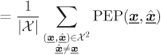

where to pass from (6.141) to (6.142) or (6.143) we use the fact that the mapping between the binary codewords ![]() and the codewords
and the codewords ![]() or
or ![]() is bijective. In a similar way, we can bound the BEP in (6.133) as
is bijective. In a similar way, we can bound the BEP in (6.133) as

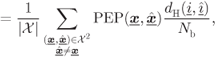
where ![]() and
and ![]() are the sequences of information bits corresponding to the codewords
are the sequences of information bits corresponding to the codewords ![]() and
and ![]() , respectively.
, respectively.
We emphasize that while the equations for the coded and uncoded cases are very similar, the PEP depends on the metrics used for decoding. In the following sections we show how these metrics affect the calculation of the PEP.
6.2.2 Expurgated Bounds
For uncoded transmission, we have already seen in Example 6.12 that PEP-based bounds such as those in (6.141) and (6.144) may be quite loose and to tighten them it is possible to remove or expurgate some terms from the bound. This expurgation strategy can be extended to the case of coded transmission, which we show below.
We start by re-deriving (6.141) in a more convenient form. To this end, we write (6.132) as
We note that
and thus, applying a union bound to (6.146) we obtain

where the inequality in (6.148) follows from the fact that, in general, the sets ![]() in the right-hand side (r.h.s.) of (6.147) are not disjoint. The general idea of expurgating the bound consists then in eliminating redundant sets in the r.h.s. of (6.147), while maintaining an inequality in (6.148). In other words, we aim at reducing the number of terms in the r.h.s. of (6.148), and by doing so, we tighten the bound on the WEP. We consider here decoders for which the decoding metric
in the right-hand side (r.h.s.) of (6.147) are not disjoint. The general idea of expurgating the bound consists then in eliminating redundant sets in the r.h.s. of (6.147), while maintaining an inequality in (6.148). In other words, we aim at reducing the number of terms in the r.h.s. of (6.148), and by doing so, we tighten the bound on the WEP. We consider here decoders for which the decoding metric ![]() can be expressed as
can be expressed as
In fact, in view of (3.7) and (3.23), we can conclude that the decoding metrics of the ML and BICM decoders can both be expressed as in (6.149).
For decoders with decoding metric in the form of (6.149), the sets ![]() can be expressed as
can be expressed as
where

We assume that the codeword ![]() can be expressed as
can be expressed as ![]() , where the binary error codewords
, where the binary error codewords ![]() and
and ![]() are orthogonal (i.e.,
are orthogonal (i.e., ![]() ). We also assume that
). We also assume that ![]() and
and ![]() are codewords. Because of the orthogonality of
are codewords. Because of the orthogonality of ![]() and
and ![]() , the codewords
, the codewords ![]() and
and ![]() differ with
differ with ![]() at different time instants, and thus, we can decompose (6.152) as
at different time instants, and thus, we can decompose (6.152) as
This allows us to conclude that if ![]() , then either
, then either ![]() or
or ![]() , which also means that if the condition
, which also means that if the condition ![]() is satisfied then either
is satisfied then either ![]() or
or ![]() is satisfied. We then immediately obtain
is satisfied. We then immediately obtain
From (6.154), we conclude that if the sets ![]() ,
, ![]() , and
, and ![]() all appear in the r.h.s. of (6.147), the set
all appear in the r.h.s. of (6.147), the set ![]() is redundant and can be removed from the union. Therefore, the term
is redundant and can be removed from the union. Therefore, the term ![]() can be removed from (6.148), and thus, the bound is tightened.
can be removed from (6.148), and thus, the bound is tightened.
The above considerations were made using only two codewords ![]() and
and ![]() ; however, they straightforwardly generalize to the case where the codewords are defined via
; however, they straightforwardly generalize to the case where the codewords are defined via ![]() orthogonal error codewords
orthogonal error codewords ![]() . In such a case, if we can write
. In such a case, if we can write ![]() , and
, and ![]() , then the contribution of
, then the contribution of ![]() can be expurgated.
can be expurgated.
6.2.3 ML Decoder
The ML decoder chooses the codeword via (3.9), and thus, the metric in (6.129) is
where (6.156) follows from (2.28). The PEP is then calculated as
where
and
For known ![]() ,
, ![]() and
and ![]() , we see from (6.162) that
, we see from (6.162) that ![]() are independent Gaussian random variables with PDF given by
are independent Gaussian random variables with PDF given by
This explains the notation ![]() , i.e.,
, i.e., ![]() has the same distribution as an L-value conditioned on transmitting a bit
has the same distribution as an L-value conditioned on transmitting a bit ![]() using binary modulation with symbols
using binary modulation with symbols ![]() and
and ![]() ; see (3.63) and (3.64).
; see (3.63) and (3.64).
In the case of nonfading channels, i.e., when ![]() , we easily see that
, we easily see that ![]() is also a Gaussian random variable with PDF
is also a Gaussian random variable with PDF
Thus, similarly to (6.79),
In fading channels, i.e., when ![]() is modeled as a random variable
is modeled as a random variable ![]() , the analysis is slightly more involved so we postpone it to Section 6.3.4.
, the analysis is slightly more involved so we postpone it to Section 6.3.4.
Since the PEP in (6.166) is a function of the Euclidean distance (ED) between the codewords only, in what follows, we define the Euclidean distance spectrum (EDS) of the code ![]() and the input-dependent Euclidean distance spectrum (IEDS) of the respective coded modulation (CM) encoder.
and the input-dependent Euclidean distance spectrum (IEDS) of the respective coded modulation (CM) encoder.
We note here the analogy between the EDS ![]() in (6.167) and the distance spectrum (DS)
in (6.167) and the distance spectrum (DS) ![]() of the code
of the code ![]() in (2.105) (cf. also
in (2.105) (cf. also ![]() in (6.168) and
in (6.168) and ![]() in (2.111)). The difference is that the index
in (2.111)). The difference is that the index ![]() in
in ![]() has a meaning of ED, while in
has a meaning of ED, while in ![]() it denotes HD. We also emphasize that the IEDS is a property of the CM encoder (i.e., it depends on how the information sequences are mapped to the symbol sequences) while the EDS is solely a property of the code
it denotes HD. We also emphasize that the IEDS is a property of the CM encoder (i.e., it depends on how the information sequences are mapped to the symbol sequences) while the EDS is solely a property of the code ![]() .
.
Now, combining (6.142) with (6.166), we obtain the following upper bound on the WEP for ML decoders:
Similarly, using (6.145), the BEP is bounded as
At this point, it is interesting to compare the WEP bound in (6.170) with the one in (6.178) (cf. also (6.172) and (6.179)). In particular, we note that ![]() in (6.170) does not enumerate all the codewords in the code
in (6.170) does not enumerate all the codewords in the code ![]() (but
(but ![]() does). Specifically, the codewords
does). Specifically, the codewords ![]() corresponding to a path in the trellis that diverged from
corresponding to a path in the trellis that diverged from ![]() , converged, and then diverged and converged again, are not taken into account in
, converged, and then diverged and converged again, are not taken into account in ![]() (while they are counted in
(while they are counted in ![]() ). However, because
). However, because ![]() (where
(where ![]() and
and ![]() are orthogonal and correspond to two diverging terms),
are orthogonal and correspond to two diverging terms), ![]() and
and ![]() are all codewords, from the analysis outlined in Section 6.2.2 we know that removing the contribution of
are all codewords, from the analysis outlined in Section 6.2.2 we know that removing the contribution of ![]() only tightens thebound.8 Consequently, (6.178) and (6.179) may be treated as expurgated bounds and we may write
only tightens thebound.8 Consequently, (6.178) and (6.179) may be treated as expurgated bounds and we may write
where the approximation is due to the expurgation.
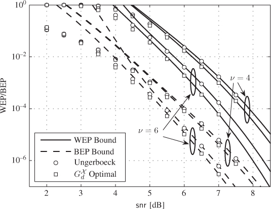
Figure 6.12 WEP and BEP bounds (lines) in (6.178) and (6.179) and simulations (markers) for Ungerboeck's encoders and CENCs optimal in terms of  for
for  ,
,  PAM,
PAM,  , and
, and 