
Chapter 3
Decoding
As explained in Chapter 2, the information bits that were mapped onto the codewords need to be correctly recovered at the receiver. This is the very essence of data transmission, where the role of the receiver is to “decode” the information bits contained in the received signals.
This chapter studies different decoding strategies and is organized as follows. The optimal maximum a posteriori (MAP) and maximum likelihood (ML) decoding strategies are introduced in Section 3.1 where we also introduce the L-values which become a key element used throughout this book. The bit-interleaved coded modulation (BICM) decoder is defined in Section 3.2. In Section 3.3, some important properties of L-values are discussed and we conclude with a discussion about hard-decision decoding in Section 3.4.
3.1 Optimal Decoding
In this section, we review well-known decoding rules. They will be compared in Section 3.2 to the BICM decoding rule, which will be based on the L-values which we will define shortly.
The logarithm is used in (3.2) to remove an exponential function which will ultimately appear in the expressions when a Gaussian channel is considered. As the logarithm is a monotonically increasing function, it does not change the maximization result in (3.1).
From Bayes' rule we obtain

where the factorization into the product of ![]() conditional channel transition probabilities is possible thanks to the assumption of transmission over a memoryless channel. Using the fact that
conditional channel transition probabilities is possible thanks to the assumption of transmission over a memoryless channel. Using the fact that ![]() in (3.3) does not depend on
in (3.3) does not depend on ![]() , we can express (3.2) as
, we can express (3.2) as
Throughout this book, the information bits are assumed to be independent and uniformly distributed (i.u.d.). This, together with the one-to-one mapping performed by the coded modulation (CM) encoder (see Section 2.2 for more details), means that the codewords ![]() are equiprobable. This leads to the definition of the ML decoding rule.
are equiprobable. This leads to the definition of the ML decoding rule.
As the mapping between code bits and symbols is bijective and memoryless (at a symbol level), we can write the ML rule in (3.6) at a bit level as
For the additive white Gaussian noise (AWGN) channel with conditional channel transition probabilities given in (2.31), the optimal decoding rule in (3.7) can be expressed as
where ![]() .
.
As the optimal operation of the decoder relies on exhaustive enumeration of the codewords via operators ![]() or
or ![]() , the expressions we have shown are entirely general, and do not depend on the structure of the encoder. Moreover, we can express the ML decoding rule in the domain of the codewords generated by the binary encoder, i.e.,
, the expressions we have shown are entirely general, and do not depend on the structure of the encoder. Moreover, we can express the ML decoding rule in the domain of the codewords generated by the binary encoder, i.e.,
where ![]() is defined in Section 2.3.3.
is defined in Section 2.3.3.
The decoding solution in (3.19) is indeed appealing: if the decoder is fed with the deinterleaved metrics ![]() , it remains unaware of the form of the mapper
, it remains unaware of the form of the mapper ![]() , the channel model, noise distribution, demapper, and so on. In other words, the metrics
, the channel model, noise distribution, demapper, and so on. In other words, the metrics ![]() act as an “interface” between the channel outcomes
act as an “interface” between the channel outcomes ![]() and the decoder. We call these metrics L-values and they are a core element in BICM decoding and bit-level information exchange. The underlying assumption for optimality of the processing based on the L-values is that the observations associated with each transmitted bit are independent (allowing us to pass from (3.11) to (3.12)). Of course, this assumption does not hold in general, nevertheless, the possibility of bit-level operation, and binary decoding in particular, may outweigh the eventual suboptimality of the resulting processing.
and the decoder. We call these metrics L-values and they are a core element in BICM decoding and bit-level information exchange. The underlying assumption for optimality of the processing based on the L-values is that the observations associated with each transmitted bit are independent (allowing us to pass from (3.11) to (3.12)). Of course, this assumption does not hold in general, nevertheless, the possibility of bit-level operation, and binary decoding in particular, may outweigh the eventual suboptimality of the resulting processing.
We note that most of the encoders/decoders used in practice are designed and analyzed using the simple transmission model of Example 3.3. In this way, the design of the encoder/decoder is done in abstraction of the observation ![]() , which allows the designer to use well-studied and well-understood off-the-shelf binary encoders/decoders. The price to pay for the resulting design simplicity is that, when the underlying assumptions of the channel are not correct, the design is suboptimal. The optimization of the encoders taking into account the underlying channel for various transmission parameters are at the heart of Chapter 8.
, which allows the designer to use well-studied and well-understood off-the-shelf binary encoders/decoders. The price to pay for the resulting design simplicity is that, when the underlying assumptions of the channel are not correct, the design is suboptimal. The optimization of the encoders taking into account the underlying channel for various transmission parameters are at the heart of Chapter 8.
3.2 BICM Decoder
As we have seen in Example 3.3, the decoding may be carried out optimally using L-values. This is the motivation for the following definition of the BICM decoder.
Using (3.17), the BICM decoding rule in (3.20) can be expressed as
which, compared to the optimal ML rule in (3.7), allows us to conclude that the BICM decoder uses the following approximation:
As (3.24) shows, the decoding metric in BICM is, in general, not proportional to ![]() , and thus, the BICM decoder can be seen as a mismatched version of the ML decoder in (3.7). Furthermore, (3.24) shows that the BICM decoder assumes that
, and thus, the BICM decoder can be seen as a mismatched version of the ML decoder in (3.7). Furthermore, (3.24) shows that the BICM decoder assumes that ![]() is not affected by the bits
is not affected by the bits ![]() . The approximation becomes the identity if the bits
. The approximation becomes the identity if the bits ![]() are independently mapped into each of the dimensions of the constellation
are independently mapped into each of the dimensions of the constellation ![]() as
as ![]() , i.e., we require
, i.e., we require ![]() , cf. Example 3.3.
, cf. Example 3.3.
The principal motivation for using the BICM decoder in Definition 3.4 is due to the bit-level operation (i.e., the binary decoding). While, as we said, this decoding rule is ML-optimal only in particular cases, cf. Example 3.3, the possibility of using any binary decoder most often outweighs the eventual decoding mismatch/suboptimality.
We note also that we might have defined the BICM decoder via likelihoods as in (3.23); however, defining it in terms of L-values as in (3.20) does not entail any loss and is simpler to implement because (i) we avoid dealing with very small numbers appearing when likelihoods are multiplied and (ii) we move the formulation to the logarithmic domain, so that the decoder uses additions instead of multiplications, which are simpler to implement.
As we will see, the expression in (3.20) is essential to analyze the performance of the BICM decoder. It will be used in Chapter 6 to study its error probability and in Chapter 7 to study the correction of suboptimal L-values. We will also use it in Chapter 8 to study unequal error protection (UEP).
3.3 L-values
In BICM, the L-values are calculated at the receiver and are used to convey information about the a posteriori probability of the transmitted bits. These signals are then used by the BICM decoder as we explain in Section 3.2.
The logarithmic likelihood ratio (LLR) or L-value for the ![]() th bit in the
th bit in the ![]() th transmitted symbol is given by
th transmitted symbol is given by
where the a posteriori and a priori L-values are, respectively, defined as
We note that unlike ![]() and
and ![]() ,
, ![]() in (3.32) does not include a time index
in (3.32) does not include a time index ![]() . This is justified by the model imposed on the bits
. This is justified by the model imposed on the bits ![]() , namely, that
, namely, that ![]() are independent and identically distributed (i.i.d.) random variables (but possibly distributed differently across the bit positions), and thus,
are independent and identically distributed (i.i.d.) random variables (but possibly distributed differently across the bit positions), and thus, ![]() . We mention that there are, nevertheless, cases when a priori information may vary with
. We mention that there are, nevertheless, cases when a priori information may vary with ![]() . This occurs in bit-interleaved coded modulation with iterative demapping (BICM-ID), where the L-value calculated by the demapper may use a priori L-values obtained from the decoder. In those cases, we will use
. This occurs in bit-interleaved coded modulation with iterative demapping (BICM-ID), where the L-value calculated by the demapper may use a priori L-values obtained from the decoder. In those cases, we will use ![]() .
.
It is well accepted to use the name LLR to refer to ![]() ,
, ![]() and
and ![]() . However, strictly speaking, only
. However, strictly speaking, only ![]() should be called an LLR. The other two quantities (
should be called an LLR. The other two quantities (![]() and
and ![]() ) are a logarithmic ratio of a posteriori probabilities and a logarithmic ratio of a priori probabilities, respectively, and not likelihood ratios. That is why using the name “L-value” to denote
) are a logarithmic ratio of a posteriori probabilities and a logarithmic ratio of a priori probabilities, respectively, and not likelihood ratios. That is why using the name “L-value” to denote ![]() ,
, ![]() and
and ![]() is convenient and avoids confusion. Furthermore, the L-value in (3.30) is sometimes called an extrinsic L-value to emphasize that it is calculated from the channel outcome without information about the a priori distribution of the bit the L-value is being calculated for.
is convenient and avoids confusion. Furthermore, the L-value in (3.30) is sometimes called an extrinsic L-value to emphasize that it is calculated from the channel outcome without information about the a priori distribution of the bit the L-value is being calculated for.
To alleviate the notation, from now on we remove the time index ![]() , i.e., the dependence of the L-values on
, i.e., the dependence of the L-values on ![]() will remain implicit unless explicitly mentioned. Using (3.29) and the fact that
will remain implicit unless explicitly mentioned. Using (3.29) and the fact that ![]() , we obtain the following relation between the a posteriori probabilities of
, we obtain the following relation between the a posteriori probabilities of ![]() and its L-value
and its L-value ![]()
An analogous relationship links the a priori L-value ![]() and the a priori probabilities, i.e.,
and the a priori probabilities, i.e.,
Combining (3.33) (3.35), and (3.30) we obtain
The constants ![]() , and
, and ![]() in the above equations are independent of
in the above equations are independent of ![]() . Therefore, moving operations to the logarithmic domain highlights the relationship between the L-values and corresponding probabilities and/or the likelihood; this relationship, up to a proportionality factor, is in the same form for a priori, a posteriori, and extrinsic L-values.
. Therefore, moving operations to the logarithmic domain highlights the relationship between the L-values and corresponding probabilities and/or the likelihood; this relationship, up to a proportionality factor, is in the same form for a priori, a posteriori, and extrinsic L-values.
We note that the L-values in (3.29) may alternatively be defined as
which could have some advantages in practical implementations. For example, in a popular complement-to-two binary format, the most significant bit (MSB) carries the sign, i.e., when an MSB is equal to zero (![]() ), it means that a number is positive, and when an MSB is equal to one (
), it means that a number is positive, and when an MSB is equal to one (![]() ), it means that the number is negative. Then, if (3.39) is used, the transmitted bit obtained via hard decisions can be recovered directly from the MSB. This, of course, has no impact on any theoretical consideration, and thus, we will always use the definition (3.29).
), it means that the number is negative. Then, if (3.39) is used, the transmitted bit obtained via hard decisions can be recovered directly from the MSB. This, of course, has no impact on any theoretical consideration, and thus, we will always use the definition (3.29).

Figure 3.1 A posteriori probabilities  as a function of the L-value
  . The thick-line portion of the plot corresponds to the function (3.45)
Assuming that the bits ![]() are independent2 (see (2.72)), the L-values in (3.29) for the AWGN channel with conditional probability density function (PDF) given by (2.31) can be calculated as
are independent2 (see (2.72)), the L-values in (3.29) for the AWGN channel with conditional probability density function (PDF) given by (2.31) can be calculated as
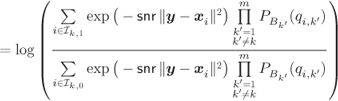

where ![]() is the
is the ![]() th bit of the labeling of the symbol
th bit of the labeling of the symbol ![]() and
and ![]() is the a priori information given by (3.32). To pass from (3.47) to (3.48), we used (2.74), and to pass from (3.48) to (3.49), we used (3.33) and the fact that the denominator of (3.33) does not depend on
is the a priori information given by (3.32). To pass from (3.47) to (3.48), we used (2.74), and to pass from (3.48) to (3.49), we used (3.33) and the fact that the denominator of (3.33) does not depend on ![]() .
.
The expression (3.49) shows us how the extrinsic L-values are calculated for the ![]() th bit in the symbol, from both the received symbol
th bit in the symbol, from both the received symbol ![]() and the available a priori information
and the available a priori information ![]() for
for ![]() . When the code bits
. When the code bits ![]() are nonuniformly distributed, the a priori L-values are obtained from the a priori distributions of the bits. Alternatively,
are nonuniformly distributed, the a priori L-values are obtained from the a priori distributions of the bits. Alternatively, ![]() could be obtained from the decoder, which is shown by the dotted lines in Fig. 2.7. When this feedback loop is present, the BICM system is referred to as BICM-ID. In BICM-ID, the decoding is performed in an iterative fashion by exchanging L-values between the decoder and the demapper.
could be obtained from the decoder, which is shown by the dotted lines in Fig. 2.7. When this feedback loop is present, the BICM system is referred to as BICM-ID. In BICM-ID, the decoding is performed in an iterative fashion by exchanging L-values between the decoder and the demapper.
When the feedback loop is not present in Fig. 2.7, the system is called a noniterative BICM, or simply BICM. In this case, the demapper computes the L-values, which are passed to the deinterleaver and then to the decoder, which produces an estimate of the information sequence ![]() . When the bits are uniformly distributed, the extrinsic L-values are calculated as
. When the bits are uniformly distributed, the extrinsic L-values are calculated as
This expression shows how the demapper ![]() computes the L-values, which depends on the received signal
computes the L-values, which depends on the received signal ![]() , the constellation and its binary labeling, and the SNR.
, the constellation and its binary labeling, and the SNR.
Having clarified the importance of the L-values for the decoding, we will now have a closer look at their properties and models. A detailed probabilistic modeling of the L-values is covered in Chapter 5.
3.3.1 PDF of L-values for Binary Modulation
The L-value ![]() in (3.50) is a function of the received symbol
in (3.50) is a function of the received symbol ![]() . For a given transmitted symbol
. For a given transmitted symbol ![]() , the received symbol
, the received symbol ![]() is a random variable
is a random variable ![]() , and thus, the L-value is also a random variable
, and thus, the L-value is also a random variable ![]() . In this section, we show how to compute the PDF of the L-values for an arbitrary binary modulation. These developments are an introduction to more general results we present in Chapter 5.
. In this section, we show how to compute the PDF of the L-values for an arbitrary binary modulation. These developments are an introduction to more general results we present in Chapter 5.
For notation simplicity, we use ![]() to denote the functional relationship between the L-value
to denote the functional relationship between the L-value ![]() and the (random) received symbol
and the (random) received symbol ![]() , i.e.,
, i.e., ![]() . Even though binary modulation may be analyzed in one dimension, we continue to use a vectorial notation to be consistent with the notation used in Chapter 5, where we develop PDFs of 2D constellations.
. Even though binary modulation may be analyzed in one dimension, we continue to use a vectorial notation to be consistent with the notation used in Chapter 5, where we develop PDFs of 2D constellations.
We consider binary modulation over the AWGN channel (i.e., ![]() and
and ![]() ) where the constellation
) where the constellation ![]() consists of two elements, and where the labeling is
consists of two elements, and where the labeling is ![]() , i.e.,
, i.e., ![]() and
and ![]() . In this case, (3.50) becomes
. In this case, (3.50) becomes
By introducing3
where ![]() is given by (2.39), we obtain from (3.53)
is given by (2.39), we obtain from (3.53)
Given a transmitted symbol ![]() ,
, ![]() , and thus, (3.56) can be expressed as
, and thus, (3.56) can be expressed as
As for binary modulation we have ![]() , we can express (3.60) conditioned on the transmitted bit
, we can express (3.60) conditioned on the transmitted bit ![]() as
as
To calculate the PDF of the L-value ![]() conditioned on the transmitted bit, we recognize (3.62) as a linear transformation of the Gaussian vector
conditioned on the transmitted bit, we recognize (3.62) as a linear transformation of the Gaussian vector ![]() , where
, where ![]() are i.i.d.
are i.i.d. ![]() . So we conclude that
. So we conclude that ![]() is a Gaussian random variable,
is a Gaussian random variable, ![]() .
.
where
The results in (3.63) and (3.64) show that transmitting any ![]() -dimensional binary modulation over the AWGN channel yields L-values whose PDF is Gaussian, with the parameters fully determined by the squared Euclidean distance (SED) between the two constellation points. The following example shows the results for the case
-dimensional binary modulation over the AWGN channel yields L-values whose PDF is Gaussian, with the parameters fully determined by the squared Euclidean distance (SED) between the two constellation points. The following example shows the results for the case ![]() , i.e., 2PAM (binary phase shift keying (BPSK)).
, i.e., 2PAM (binary phase shift keying (BPSK)).

Figure 3.2 The L-values for binary modulation are known to be Gaussian distributed as they are a linear transformation of a Gaussian random variable
The result in (3.63) shows that the PDF of the L-values for binary modulation is Gaussian and this form of the PDF is often used for modeling of the L-values in different contexts. In reality, the PDF is not Gaussian in the case of multilevel modulations, as we will show in Chapter 5.
3.3.2 Fundamental Properties of the L-values
In what follows, we discuss two fundamental properties of the PDF of the L-values which will become useful in the following chapters.
As we will see later, consistency is an inherent property of the L-values if they are calculated via (3.29).
We note that the practical implementation of equation (3.70) is, in general, rather tedious, as will be shown in Section 5.1.2. Another important observation is that the proof relies on the relationship ![]() obtained from (3.29), and thus, it does not hold for max-log (or any other kind of approximated) L-values.
obtained from (3.29), and thus, it does not hold for max-log (or any other kind of approximated) L-values.
The consistency condition is an inherent property of the PDF of an L-value, but there is another property important for the analysis: the symmetry.
Clearly, a necessary condition for a PDF to satisfy the symmetry condition is that its support is symmetric with respect to zero.
The symmetry condition in Definition 3.11 can be seen as a “natural” extension of the symmetry of the 2PAM case in Example 3.12. As we will see, this condition is not always satisfied; however, it it is convenient to enforce it as then, the analysis of the BICM receiver is simplified. To this end, we assume that before being passed to the mapper, the bits ![]() are scrambled, as shown in Fig. 3.3, i.e., the bits at the input of the mapper are a result of a binary exclusive OR (XOR) operation
are scrambled, as shown in Fig. 3.3, i.e., the bits at the input of the mapper are a result of a binary exclusive OR (XOR) operation
with bits ![]() generated in a pseudorandom manner. We model these scrambled bits as i.i.d. random variables
generated in a pseudorandom manner. We model these scrambled bits as i.i.d. random variables ![]() with
with ![]() .
.

Figure 3.3 The sequence of pseudorandom bits  is known by the scrambler
  and the descrambler
  . The dashed-dotted boxes indicate that these two processing units may be considered as a part of the mapper and demapper
We assume that both the transmitter and the receiver know the scrambling sequence ![]() , as schematically shown in Fig. 3.3. Thus, the “scrambling” and the “descrambling” may be considered, respectively, as part of the mapper and the demapper, and consequently, are not shown in the BICM block diagrams. In fact, the scrambling we described is often included in practical communication systems.
, as schematically shown in Fig. 3.3. Thus, the “scrambling” and the “descrambling” may be considered, respectively, as part of the mapper and the demapper, and consequently, are not shown in the BICM block diagrams. In fact, the scrambling we described is often included in practical communication systems.
The L-values at the output of the descrambler can be expressed as
which gives
where ![]() is the L-value obtained for the bits
is the L-value obtained for the bits ![]() . From (3.81), we see that the operation of the descrambler simply corresponds to changing the sign of the L-value
. From (3.81), we see that the operation of the descrambler simply corresponds to changing the sign of the L-value ![]() according to the scrambling sequence.
according to the scrambling sequence.
Thus, thanks to the scrambler, the PDF of the L-values ![]() in Fig. 3.3 are symmetric regardless of the form of the PDF
in Fig. 3.3 are symmetric regardless of the form of the PDF ![]() . In analogy to the above development, we conclude that the joint symmetry condition (3.75) is also satisfied if the scrambler is used.
. In analogy to the above development, we conclude that the joint symmetry condition (3.75) is also satisfied if the scrambler is used.
The symmetry-consistency condition (also referred to as the exponential symmetric condition) in Definition 3.14 will be used in Chapters 6 and 7. Clearly, the PDF of the L-values for 2PAM fulfills this condition.
3.3.3 Approximations
The computation of ![]() in (3.50) involves computing (
in (3.50) involves computing (![]() times) the function
times) the function ![]() . To deal with the exponential increase of the complexity as
. To deal with the exponential increase of the complexity as ![]() grows, approximations are often used. One of the most common approaches stems from the factorization of the logarithm of a sum of exponentials via the so-called Jacobian logarithm, i.e.,
grows, approximations are often used. One of the most common approaches stems from the factorization of the logarithm of a sum of exponentials via the so-called Jacobian logarithm, i.e.,
where
with
The function ![]() in (3.94) is shown in Fig. 3.4.
in (3.94) is shown in Fig. 3.4.

Figure 3.4 The function  in (3.94) and the two approximations in Example 3.16
The “max-star” operation in (3.93) can be applied recursively to more than two arguments, i.e.,
The advantage of using (3.95) is that the function ![]() in (3.94) fulfills
in (3.94) fulfills ![]() , and thus, can be efficiently implemented via a lookup table or via an analytical approximation based on piecewise linear functions. This is interesting from an implementation point of view because the function
, and thus, can be efficiently implemented via a lookup table or via an analytical approximation based on piecewise linear functions. This is interesting from an implementation point of view because the function ![]() does not have to be explicitly evoked.
does not have to be explicitly evoked.
Example 3.16 shows two simple ways of approximating ![]() in (3.93), and in general, other simplifications can be devised. Arguably, the simplest approximation is obtained ignoring
in (3.93), and in general, other simplifications can be devised. Arguably, the simplest approximation is obtained ignoring ![]() , i.e., setting
, i.e., setting ![]() which used in (3.95) yields the popular max-log approximation
which used in (3.95) yields the popular max-log approximation
By using (3.98) in (3.50), we obtain the following approximation for the L-values
which are usually called max-log L-values.
Although the max-log L-values in (3.99) are suboptimal, they are frequently used in practice. One reason for their popularity is that some arithmetic operations are removed, and thus, the complexity of the L-values calculation is reduced. This is relevant from an implementation point of view and it explains why the max-log approach was recommended by the third-generation partnership project (3GPP) working groups. Most of the analysis and design of BICM transceivers in this book will be based onmax-log L-values, which we will simply call L-values, despite their suboptimal calculation.
It is worthwhile mentioning that the max-log approximation given by (3.98) as well as the max-star approximation in (3.93) can also be used in the decoding algorithms of turbo codes (TCs), i.e., in the soft-input soft-output blocks described in Section 2.6.3. When MAP decoding is implemented in the logarithmic domain (Log-MAP) using the Bahl–Cocke–Jelinek–Raviv (BCJR) algorithm, computations involving logarithms of sum of terms appear. Consequently, the max-star and max-log approximations can be used to reduce the decoding complexity, which yields the Max-Log-MAP algorithm. Different approaches for simplified metric calculation have been investigated in the literature, for both the decoding algorithm and the metric calculation in the demapper. Some of the issues related to optimizing the simplified metrics' calculation in the demapper will be addressed in Chapter 7.
Another interesting feature of the max-log approximation will become apparent on the basis of the discussion in Section 3.2. As we showed in (3.20), the decisions made by a BICM decoder are based on calculating linear combinations of the L-values. Then, a linear scaling of all the L-values by a common factor is irrelevant to the decoding decision, so we may remove the factor ![]() in (3.99) without affecting the decoding results. Consequently, the receiver does not need to estimate the noise variance
in (3.99) without affecting the decoding results. Consequently, the receiver does not need to estimate the noise variance ![]() . The family of decoders that are insensitive to a linear scaling of their inputs includes, e.g., the Viterbi algorithm and the Max-Log-MAP turbo decoder. However, the
. The family of decoders that are insensitive to a linear scaling of their inputs includes, e.g., the Viterbi algorithm and the Max-Log-MAP turbo decoder. However, the ![]() factor should still be considered if the decoder processes the L-values in a nonlinear manner, e.g., when the true MAP decoding algorithm is used.
factor should still be considered if the decoder processes the L-values in a nonlinear manner, e.g., when the true MAP decoding algorithm is used.
While the reasons above are more of a practical nature, there are other more theoretical reasons for considering the max-log approximation. The first one is that max-log L-values are asymptotically tight, i.e., when one of the SEDs ![]() is (on average) very small compared to the others (i.e., when
is (on average) very small compared to the others (i.e., when ![]() ), there is no loss in only considering the dominant exponential function. Another reason favoring the max-log approximation is that, although suboptimal, it has negligible impact on the receiver's performance when Gray-labeled constellations are used.
), there is no loss in only considering the dominant exponential function. Another reason favoring the max-log approximation is that, although suboptimal, it has negligible impact on the receiver's performance when Gray-labeled constellations are used.
Finally, the max-log approximation transforms the nonlinear relation between ![]() and
and ![]() in (3.50) into a piecewise linear relation and this enables the analytical description of the L-values we show in Chapter 5.
in (3.50) into a piecewise linear relation and this enables the analytical description of the L-values we show in Chapter 5.
3.4 Hard-Decision Decoding
The decoding we have analyzed up to now is based on the channel observations ![]() or the L-values
or the L-values ![]() . This is also referred to as “soft decisions” to emphasize the fact that the reliability of the MAP estimate of the transmitted bits may be deduced from their amplitude (see Example 3.6).
. This is also referred to as “soft decisions” to emphasize the fact that the reliability of the MAP estimate of the transmitted bits may be deduced from their amplitude (see Example 3.6).
By ignoring the reliability, we may still detect the transmitted symbols/bits before decoding. This is mostly considered for historical reasons, but still may be motivated by the simplicity of the resulting processing. The idea is to transform the hard decisions on ![]() or
or ![]() into MAP estimates of the symbols/bits. Nowadays, such a “hard-decision” decoding is rather a benchmark for the widely used soft-decision decoding we are mostly interested in.
into MAP estimates of the symbols/bits. Nowadays, such a “hard-decision” decoding is rather a benchmark for the widely used soft-decision decoding we are mostly interested in.
In hard-decision symbol detection, we ignore coding, i.e., we take ![]() . From (3.11), assuming equiprobable symbols and omitting the time instant
. From (3.11), assuming equiprobable symbols and omitting the time instant ![]() , we obtain
, we obtain
which finds the closest (in terms of Euclidean distance (ED)) symbol in the constellation to the received vector ![]() , where the set of all
, where the set of all ![]() producing the decision
producing the decision ![]() is called the Voronoi region of the symbol
is called the Voronoi region of the symbol ![]() ,
, ![]() (discussed in greater detail in Chapter 6).
(discussed in greater detail in Chapter 6).
Once hard decisions are made via (3.100), we obtain the sequence of symbol estimates ![]() , which can be seen as a discretization of the received signal
, which can be seen as a discretization of the received signal ![]() . The discretized sequence of received signals can still be used for decoding the transmitted sequence in an ML sense. To this end, the obtained estimates
. The discretized sequence of received signals can still be used for decoding the transmitted sequence in an ML sense. To this end, the obtained estimates ![]() should be considered the observations and modeled as random variables (because they are functions of the random variable
should be considered the observations and modeled as random variables (because they are functions of the random variable ![]() ) with the conditional probability mass function (PMF)
) with the conditional probability mass function (PMF)
The ML sequence decoding using the hard decisions ![]() is then obtained using (3.101) in (3.6), i.e.,
is then obtained using (3.101) in (3.6), i.e.,
While we can use the hard decisions to perform ML sequence decoding, this remains a suboptimal approach due to the loss of information in the discretization of the signals ![]() to
to ![]() points (when going from
points (when going from ![]() to
to ![]() via (3.100)).
via (3.100)).
In the same way that we considered hard-decision symbol detection, we may consider the BICM decoder in (3.20) when hard decisions on the transmitted bits are made according to (3.40). Formulating the problem in the optimal framework of Section 3.1, the ML sequence decoding is given by
The decision rule in (3.103) uses the “observations” ![]() in an optimal way, but is not equivalent to the sequence decoding (3.102) because
in an optimal way, but is not equivalent to the sequence decoding (3.102) because ![]() . As we will see, the equivalence occurs only when making a decision from the max-log L-values.
. As we will see, the equivalence occurs only when making a decision from the max-log L-values.
The decision rule in (3.103) uses the observations ![]() in an ML sense, and thus, is optimal. On the other hand, if we want to use a BICM decoder (i.e., L-values passed to the deinterleaver followed by decoding), we need to transform the hard decisions on the bits
in an ML sense, and thus, is optimal. On the other hand, if we want to use a BICM decoder (i.e., L-values passed to the deinterleaver followed by decoding), we need to transform the hard decisions on the bits ![]() into “hard-decision” L-values. To this end, we use (3.29) with
into “hard-decision” L-values. To this end, we use (3.29) with ![]() as the observations, i.e.,
as the observations, i.e.,
The hard-decision L-values in (3.107) are a binary representation of the reliability of the hard decisions made on the bits, and can be expressed as

where the bit-error probability (BEP) for the ![]() th bit is defined as
th bit is defined as
The BEP in (3.110) is an unconditional BEP (i.e., not the same as the conditional BEP in (3.41)) which can be calculated using methods described in Section 6.1.1.
3.5 Bibliographical Notes
BICM was introduced in [1], where it was shown that despite the suboptimality of the BICM decoder, BICM transmission provides diversity gains in fading channels. This spurred the interest in the BICM decoding principle which was later studied in detail in [2–4].
The symmetry-consistency condition of the L-values appeared in [5] and was later used in [6], for example. The symmetry condition for the channel and the decoding algorithm was studied in [7]. The symmetry and consistency conditions were also described in [8, Section III]. The idea of scrambling the bits to “symmetrize” the channel was already postulated in [2] and it is nowadays a conventional assumption when studying the performance of BICM.
The use of the max-star/max-log approximation has been widely used from the 1990s for both the decoding algorithm and the metrics calculation in the demapper (see, e.g., [9–15] and references therein). This simplification, proposed already in the original BICM paper [1] has also been proposed by the 3GPP working groups [16]. The small losses caused by using the max-log approximation with Gray-labeled constellations has been reported in [17, Fig. 9; 18].
Recognizing the BICM decoder as a mismatched decoder [19–21] is due to [22] where the generalized mutual information (GMI) was shown to be an achievable rate for BICM (discussed in greater detail in Section 4.3). Mismatched metrics for BICM have also been studied in [23 24]. The equivalence between the bitwise hard decisions based on max-log L-values and the symbolwise decisions was briefly mentioned in [25, Section IV-A] and proved in [26, Section II-C] (see also [27]).
References
- [1] Zehavi, E. (1992) 8-PSK trellis codes for a Rayleigh channel. IEEE Trans. Commun., 40 (3), 873–884.
- [2] Caire, G., Taricco, G., and Biglieri, E. (1998) Bit-interleaved coded modulation. IEEE Trans. Inf. Theory, 44 (3), 927–946.
- [3] Wachsmann, U., Fischer, R. F. H., and Huber, J. B. (1999) Multilevel codes: theoretical concepts and practical design rules. IEEE Trans. Inf. Theory, 45 (5), 1361–1391.
- [4] Guillén i Fàbregas, A., Martinez, A., and Caire, G. (2008) Bit-interleaved coded modulation. Found. Trends Commun. Inf. Theory, 5 (1–2), 1–153.
- [5] Hoeher, P., Land, I., and Sorger, U. (2000) Log-likelihood values and Monte Carlo simulation—some fundamental results. In Proceedings International Symposium on Turbo Codes and Related Topics, September 2000, Brest, France.
- [6] ten Brink, S. (2001) Convergence behaviour of iteratively decoded parallel concatenated codes. IEEE Trans. Commun., 49 (10), 1727–1737.
- [7] Richardson, T. J. and Urbanke, R. L. (2001) The capacity of low-density-parity-check codes under message-passing decoding. IEEE Trans. Inf. Theory, 47 (2), 599–618.
- [8] Tüchler, M. (2004) Design of serially concatenated systems depending on the block length. IEEE Trans. Commun., 52 (2), 209–218.
- [9] Viterbi, A. J. (1998) An intuitive justification and a simplified implementation of the MAP decoder for convolutional codes. IEEE J. Sel. Areas Commun., 16 (2), 260–264.
- [10] Robertson, P., Villebrun, E., and Hoeher, P. (1995) A comparison of optimal and sub-optimal MAP decoding algorithms operating in the log domain. IEEE International Conference on Communications (ICC), June 1995, Seattle, WA.
- [11] Pietrobon, S. S. (1995) Implementation and performance of a serial MAP decoder for use in an iterative turbo decoder. IEEE International Symposium on Information Theory (ISIT), September 1995, Whistler, BC, Canada.
- [12] Benedetto, S., Divsalar, D., Montorsi, G., and Pollara, F. (1995) Soft-output decoding algorithms in iterative decoding of turbo codes. TDA Progress Report 42-87, Jet Propulsion Laboratory, Pasadena, CA, pp. 63–121.
- [13] Gross, W. and Gulak, P. (1998) Simplified MAP algorithm suitable for implementation of turbo decoders. Electron. Lett., 34 (16), 1577–1578.
- [14] Valenti, M. and Sun, J. (2001) The UMTS turbo code and an efficient decoder implementation suitable for software defined radios. Int. J. Wirel. Inf. Netw., 8 (4), 203–216.
- [15] Hu, X.-Y., Eleftheriou, E., Arnold, D.-M., and Dholakia, A. (2001) Efficient implementations of the sum-product algorithm for decoding LDPC codes. IEEE Global Telecommunications Conference (GLOBECOM), November 2001, San Antonio, TX.
- [16] Ericsson, Motorola, and Nokia (2000) Link evaluation methods for high speed downlink packet access (HSDPA). TSG-RAN Working Group 1 Meeting #15, TSGR1#15(00)1093, Tech. Rep., August 2000.
- [17] Classon, B., Blankenship, K., and Desai, V. (2002) Channel coding for 4G systems with adaptive modulation and coding. IEEE Wirel. Commun. Mag., 9 (2), 8–13.
- [18] Alvarado, A., Carrasco, H., and Feick, R. (2006) On adaptive BICM with finite block-length and simplified metrics calculation. IEEE Vehicular Technology Conference (VTC-Fall), September 2006, Montreal, QC, Canada.
- [19] Ganti, A., Lapidoth, A., and Telatar, I. E. (2000) Mismatched decoding revisited: general alphabets, channels with memory, and the wide-band limit. IEEE Trans. Inf. Theory, 46 (7), 2315–2328.
- [20] Kaplan, G. and Shamai, S. (Shitz) (1993) Information rates and error exponents of compound channels with application to antipodal signaling in a fading environment. Archiv fuer Elektronik und Uebertragungstechnik, 47 (4), 228–239.
- [21] Merhav, N., Kaplan, G., Lapidoh, A., and Shamai (Shitz), S. (1994) On information rates for mismatched decoders. IEEE Trans. Inf. Theory, 40 (6), 1953–1967.
- [22] Martinez, A., Guillén i Fàbregas, A., Caire, G., and Willems, F. M. J. (2009) Bit-interleaved coded modulation revisited: A mismatched decoding perspective. IEEE Trans. Inf. Theory, 55 (6), 2756–2765.
- [23] Nguyen, T. and Lampe, L. (2011) Bit-interleaved coded modulation with mismatched decoding metrics. IEEE Trans. Commun., 59 (2), 437–447.
- [24] Nguyen, T. and Lampe, L. (2011) Mismatched bit-interleaved coded noncoherent orthogonal modulation. IEEE Commun. Lett., 5, 563–565.
- [25] Fertl, P., Jaldén, J., and Matz, G. (2012) Performance assessment of MIMO-BICM demodulators based on mutual information. IEEE Trans. Signal Process., 60 (3), 2764–2772.
- [26] Ivanov, M., Brännström, F., Alvarado, A., and Agrell, E. (2012) General BER expression for one-dimensional constellations. IEEE Global Telecommunications Conference (GLOBECOM), December 2012, Anaheim, CA
- [27] Ivanov, M., Brännström, F., Alvarado, A., and Agrell, E. (2013) On the exact BER of bit-wise demodulators for one-dimensional constellations. IEEE Trans. Commun., 61 (4), 1450–1459.