
6.3 PEP Evaluation
From the results in Sections 6.2.4 and 6.2.5, we know that finding the PEP in (6.166) and (6.226) is instrumental to evaluate the performance of the ML and BICM decoders, respectively. In the case of the BICM decoder we need to evaluate
where
and ![]() is the average PDF given in (6.227). Alternatively, we might want to calculate
is the average PDF given in (6.227). Alternatively, we might want to calculate
where
and carry out the summation (6.233) over ![]() . Note that, to simplify the notation we removed the subindexing with
. Note that, to simplify the notation we removed the subindexing with ![]() we used in (6.210).
we used in (6.210).
Although we used the same notation in (6.283) and (6.285), the random variables ![]() described by these PDFs are not the same. In the first case, to evaluate the PEP, we have to consider only i.i.d. random variables. In the case of (6.285) the random variables are non-i.i.d.; we treat this case in Section 6.3.4.
described by these PDFs are not the same. In the first case, to evaluate the PEP, we have to consider only i.i.d. random variables. In the case of (6.285) the random variables are non-i.i.d.; we treat this case in Section 6.3.4.
6.3.1 Numerical Integration
In general, we will have to deal with distributions different from the Gaussian case we showed in Example 6.24. The direct way to obtain the tail integral of the multiple convolution is via direct and inverse Laplace-type transforms, i.e., from the relationship linking the MGF (see (2.6)) of the L-values ![]() and their PDF
and their PDF ![]() given in (6.227).13 More specifically,
given in (6.227).13 More specifically,
and
where ![]() is taken from the domain of the MGF.
is taken from the domain of the MGF.
Expressing (6.282) as
where ![]() and
and ![]() is the inverted step function with MGF
is the inverted step function with MGF ![]() . The PEP can be then calculated by inverting the MGF of
. The PEP can be then calculated by inverting the MGF of ![]() , i.e.,
, i.e.,

Finding exact analytical solutions of the integral (6.291) is often impossible so numerical integration is then used. Before studying this approach, we show a useful lemma.
In what follows, we show how to numerically calculate (6.291). To this end, we use a Gauss-Chebyshev (GCh) quadrature, which states that for any function ![]() that can be represented by polynomials for
that can be represented by polynomials for ![]() ,
,
where ![]() and
and ![]() .
.
Using the substitution ![]() , (6.291) becomes
, (6.291) becomes
where (6.297) follows from the fact that the second part of the integrand in (6.297) is odd. This is due to Lemma 6.25, which shows that ![]() is real and even.
is real and even.
After the change of variable ![]() , (6.297) becomes
, (6.297) becomes
where
Thus, using (6.294) in (6.298) yields
We then use ![]() and take advantage of the symmetry
and take advantage of the symmetry ![]() and
and ![]() . This yields the final expression for the PEP
. This yields the final expression for the PEP
where ![]() and
and ![]() is the MGF of the random variable
is the MGF of the random variable ![]() with PDF given by (6.227).
with PDF given by (6.227).
To evaluate the PEP in (6.301), one would ideally use a large value of ![]() . However, a good tradeoff between accuracy and implementation complexity is typically obtained for relatively small values of
. However, a good tradeoff between accuracy and implementation complexity is typically obtained for relatively small values of ![]() . Most of the examples in this chapter were calculated using
. Most of the examples in this chapter were calculated using ![]() or
or ![]() .
.

Figure 6.18 The real (a) and imaginary (b) parts of the MGF  in (6.303) for
  and
and  . The points along the integration line
  (shown with circles) correspond to the GCh quadrature nodes with
  . As expected (see Lemma 6.25),
  for
for 
We conclude this section by making some remarks about the PEP expression in (6.301):
- The numerical complexity grows with the number of terms required by (6.243), as the integration (6.301) must be carried out for each value of
 . This brings implementation burden when we need to evaluate
  for many different values of
  .
. - The MGF
 must be known for
  values of
  required in (6.301). While in some cases we may be able to analytically calculate the MGF from the analytical form of the PDF
  , in others, it is too cumbersome or even impossible. In fact, it may be difficult to derive tractable expressions for the PDF
  in the first place, e.g., when the L-values depend on many random parameters.
 - In the cases where the PDF is not known, we may replace (6.286) by Monte Carlo integration. To this end, we use a sum over realizations
 of
of  , conditioned on the inputs of the BICM channel in Fig. 5.1, i.e.,
6.309
, conditioned on the inputs of the BICM channel in Fig. 5.1, i.e.,
6.309 6.310
6.310
The complexity of the PEP evaluation is then dominated by (6.311), which has to be evaluated
 times for different values of
  as required by (6.301).
 - The expression (6.301) does not explicitly relate to the parameters of BICM (e.g., constellation and labeling), and thus, it does not provide insights for the design.
6.3.2 Saddlepoint Approximation
To go around the first two difficulties mentioned above, the so-called saddlepoint approximation (SPA) may be used to efficiently approximate the PEP. The SPA is a tool known in statistical analysis to efficiently calculate cumulative distribution functions (CDFs) and PDFs of a sum of random variables using the cumulant generating function (CGF)
For a sum of i.i.d. random variables such as ![]() , we obtain
, we obtain
and thus, (6.291) becomes
A formal derivation of the SPA may be found in the textbooks we reference in Section 6.5. Here, we provide an intuitive explanation for why SPA “work”. We start by approximating the CGF in (6.312) via a truncated Taylor series around ![]() , i.e.,
, i.e.,
where ![]() and
and ![]() are the first and second derivatives of the CGF given by
are the first and second derivatives of the CGF given by
The Taylor expansion in (6.315) is done around the so-called saddlepoint ![]() , chosen to satisfy
, chosen to satisfy ![]() , which used in (6.314) gives the SPA
, which used in (6.314) gives the SPA
After the change of variables ![]() we obtain
we obtain

where
and where (6.320) results from ![]() .
.
Using ![]() transforms (6.321) into
transforms (6.321) into
Alternatively, if the (tighter) approximation ![]() is used, we obtain
is used, we obtain
We can also transform the expression in (6.322) and (6.323) back into the MGF domain via (6.312). For example, (6.323) becomes
We have obtained expressions that depend solely on the MGF or CGF evaluated at ![]() . This is an important simplification when compared to (6.301), as once
. This is an important simplification when compared to (6.301), as once ![]() and
and ![]() are known, we can evaluate
are known, we can evaluate ![]() for any
for any ![]() . The caveat is that now,
. The caveat is that now, ![]() must be found. This is usually the most difficult part of the SPA method because solving nonlinear saddlepoint equation
must be found. This is usually the most difficult part of the SPA method because solving nonlinear saddlepoint equation ![]() , or equivalently
, or equivalently
is, in general, not trivial. However, for the cases we study here, it is in fact quite simple.
We note that to solve (6.325) we need to choose ![]() to satisfy
to satisfy
From (3.85) we know that the function ![]() is odd, which allows us to conclude that for
is odd, which allows us to conclude that for
the integrand in (6.326) is also odd, and thus, (6.327) solves (6.325). To show that this solution is unique, we need to demonstrate that ![]() is convex, i.e.,
is convex, i.e.,
which can be recognized as Hölder's inequality, and therefore, holds independently of the distribution of the random variable ![]() .
.
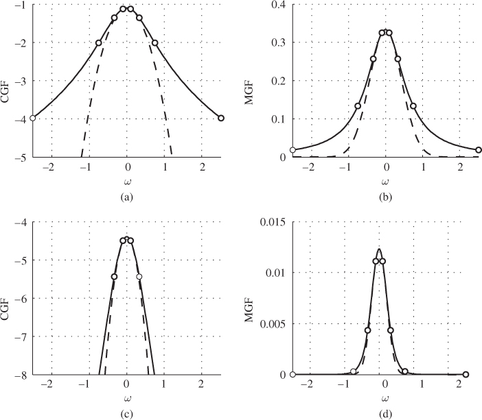
Figure 6.19 CGF  (solid lines) and its second-order approximation
  (dashed lines) are shown together with the corresponding MGF
  (solid lines) and its approximation
  (dashed lines): (a)
  , (b)
, (b)  , (c)
, (c)  , and (d)
  . The circles indicate the position of the
  quadrature nodes necessary to implement the solution from Section 6.3.1. Here
Thanks to the SPA, once we know ![]() and
and ![]() for one real argument
for one real argument ![]() , we may calculate
, we may calculate ![]() for any value of
for any value of ![]() . This stands in contrast to the numerical integration approach, where we have to evaluate the MGF for
. This stands in contrast to the numerical integration approach, where we have to evaluate the MGF for ![]() points (see (6.301)), and next carry out the summations for each
points (see (6.301)), and next carry out the summations for each ![]() . Thus, not only does the SPA allow us to obtain analytical solutions in some cases, but it also offers a clear advantage over numerical integration when the MGF is difficult to acquire.
. Thus, not only does the SPA allow us to obtain analytical solutions in some cases, but it also offers a clear advantage over numerical integration when the MGF is difficult to acquire.
6.3.3 Chernoff Bound
Another useful approximation of the PEP relies on using upper bounding techniques, as shown in the following theorem.
The proof of Theorem 6.29 shows that ![]() for any
for any ![]() . In Theorem 6.29 we use
. In Theorem 6.29 we use ![]() as this value of
as this value of ![]() minimizes
minimizes ![]() , and thus, tightens the bound (6.340).
, and thus, tightens the bound (6.340).
For the particular case of 2PAM transmission, from (6.329) we have ![]() , so the Chernoff bound in (6.336) is given by
, so the Chernoff bound in (6.336) is given by
Using ![]() , we bound the true PEP in (6.258) as
, we bound the true PEP in (6.258) as
which shows that the Chernoff bound in (6.342) goes to zero (as ![]() ) slower than the actual value of the PEP. The next example shows PEP calculation for 2PAM in fading channels.
) slower than the actual value of the PEP. The next example shows PEP calculation for 2PAM in fading channels.

Figure 6.20 Comparison of the PEP estimation methods for a 2PAM constellation in Rayleigh fading channel. To obtain  we used (6.308) with
  quadrature points
6.3.4 Nonidentically Distributed L-values
We can now revisit the assumption that the L-values ![]() entering the metric
entering the metric ![]() are identically distributed. Such an assumption is sufficient when using the model (6.227), but in the most general case (6.218), we need to calculate
are identically distributed. Such an assumption is sufficient when using the model (6.227), but in the most general case (6.218), we need to calculate ![]() in (6.284). In this case,
in (6.284). In this case, ![]() is a sum of
is a sum of ![]() random variables,
random variables, ![]() with distribution
with distribution ![]() ,
, ![]() with a distribution
with a distribution ![]() , and so on, where
, and so on, where ![]() . We denote the MGF of the
. We denote the MGF of the ![]() th distribution by
th distribution by ![]() , and its CGF by
, and its CGF by ![]() . The extension of the previously obtained formulas thus requires replacing the MGF
. The extension of the previously obtained formulas thus requires replacing the MGF ![]() with the product
with the product ![]() .
.
The numerical integration (6.301) is generalized as
The SPA-based solution (6.323) becomes
and the upper bound is generalized as
where
and thus ![]() .
.
We will exploit the bound (6.355) in Lemma 7.13 and use it in the following example to find the PEP of trellis-coded modulation (TCM) receivers.