
CHAPTER 23
Graphs.
Combinatorial Optimization

Many problems in electrical engineering, civil engineering, operations research, industrial engineering, management, logistics, marketing, and economics can be modeled by graphs and directed graphs, called digraphs. This is not surprising as they allow us to model networks, such as roads and cables, where the nodes may be cities or computers. The task then is to find the shortest path through the network or the best way to connect computers. Indeed, many researchers who made contributions to combinatorial optimization and graphs, and whose names lend themselves to fundamental algorithms in this chapter, such as Fulkerson, Kruskal, Moore, and Prim, all worked at Bell Laboratories in New Jersey, the major R&D facilities of the huge telephone and telecommunication company AT&T. As such, they were interested in methods of optimally building computer networks and telephone networks. The field has progressed into looking for more and more efficient algorithms for very large problems.
Combinatorial optimization deals with optimization problems that are of a pronounced discrete or combinatorial nature. Often the problems are very large and so a direct search may not be possible. Just like in linear programming (Chap. 22), the computer is an indispensible tool and makes solving large-scale modeling problems possible. Because the area has a distinct flavor, different from ODEs, linear algebra, and other areas, we start with the basics and gradually introduce algorithms for shortest path problems (Secs. 22.2, 22.3), shortest spanning trees (Secs. 23.4, 23.5), flow problems in networks (Secs. 23.6, 23.7), and assignment problems (Sec. 23.8).
Prerequisite: none.
References and Answers to Problems: App. 1 Part F, App. 2.
23.1 Graphs and Digraphs
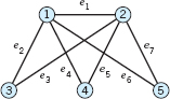
Roughly, a graph consists of points, called vertices, and lines connecting them, called edges. For example, these may be four cities and five highways connecting them, as in Fig. 477. Or the points may represent some people, and we connect by an edge those who do business with each other. Or the vertices may represent computers in a network and the edge connections between them. Let us now give a formal definition.

Fig. 477. Graph consisting of 4 vertices and 5 edges

Fig. 478. Isolated vertex, loop, double edge. (Excluded by definition.)
DEFINITION Graph
A graphG consists of two finite sets (sets having finitely many elements), a set V of points, called vertices, and a set E of connecting lines, called edges, such that each edge connects two vertices, called the endpoints of the edge. We write
![]()
Excluded are isolated vertices (vertices that are not endpoints of any edge), loops (edges whose endpoints coincide), and multiple edges (edges that have both endpoints in common). See Fig. 478.
CAUTION! Our three exclusions are practical and widely accepted, but not uniformly. For instance, some authors permit multiple edges and call graphs without them simple graphs.
We denote vertices by letters, u, ν, … or ν1, ν2, … or simply by numbers 1, 2, … (as in Fig. 477). We denote edges by e1, e2, … or by their two endpoints; for instance, e1 = (1, 4), e2 = (1, 2) in Fig. 477.
An edge (νi, νj) is called incident with the vertex νi (and conversely); similarly, (νi, νj) is incident with νj. The number of edges incident with a vertex ν is called the degree of ν. Two vertices are called adjacent in G if they are connected by an edge in G (that is, if they are the two endpoints of some edge in G).
We meet graphs in different fields under different names: as “networks” in electrical engineering, “structures” in civil engineering, “molecular structures” in chemistry, “organizational structures” in economics, “sociograms,” “road maps,” “telecommunication networks,” and so on.
Digraphs (Directed Graphs)
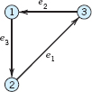
Nets of one-way streets, pipeline networks, sequences of jobs in construction work, flows of computation in a computer, producer–consumer relations, and many other applications suggest the idea of a “digraph” (= directed graph), in which each edge has a direction (indicated by an arrow, as in Fig. 479).

DEFINITION Digraph (Directed Graph)
A digraph G = (V, E) is a graph in which each edge e = (i, j) has a direction from its “initial point” i to its “terminal point” j.
Two edges connecting the same two points i, j are now permitted, provided they have opposite directions, that is, they are (i, j) and (i, j) Example. (1, 4) and (4, 1) in Fig. 479.
A subgraph or subdigraph of a given graph or digraph G = (V, E), respectively, is a graph or digraph obtained by deleting some of the edges and vertices of G, retaining the other edges of G (together with their pairs of endpoints). For instance, e1, e3 (together with the vertices 1, 2, 4) form a subgraph in Fig. 477, and e3, e4, e5 (together with the vertices 1, 3, 4) form a subdigraph in Fig. 479.
Computer Representation of Graphs and Digraphs
Drawings of graphs are useful to people in explaining or illustrating specific situations. Here one should be aware that a graph may be sketched in various ways; see Fig. 480. For handling graphs and digraphs in computers, one uses matrices or lists as appropriate data structures, as follows.
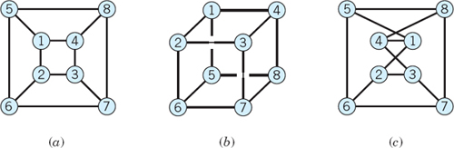
Fig. 480. Different sketches of the same graph
Adjacency Matrix of a Graph G: Matrix A = [aij] with entries
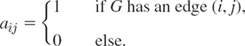
Thus aij = 1 if and only if two vertices i and j are adjacent in G. Here, by definition, no vertex is considered to be adjacent to itself; thus, aii = 0. A is symmetric, aij = aji. (Why?)
The adjacency matrix of a graph is generally much smaller than the so-called incidence matrix (see Prob. 18) and is preferred over the latter if one decides to store a graph in a computer in matrix form.

Adjacency Matrix of a Digraph G: Matrix A = [aij] with entries
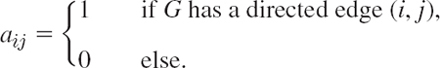
This matrix A need not be symmetric. (Why?)

Lists. The vertex incidence list of a graph shows, for each vertex, the incident edges. The edge incidence list shows for each edge its two endpoints. Similarly for a digraph; in the vertex list, outgoing edges then get a minus sign, and in the edge list we now have ordered pairs of vertices.
EXAMPLE 3 Vertex Incidence List and Edge Incidence List of a Graph
This graph is the same as in Example 1, except for notation.

Sparse graphs are graphs with few edges (far fewer than the maximum possible number n(n − 1)/2, where n is the number of vertices). For these graphs, matrices are not efficient. Lists then have the advantage of requiring much less storage and being easier to handle; they can be ordered, sorted, or manipulated in various other ways directly within the computer. For instance, in tracing a “walk” (a connected sequence of edges with pairwise common endpoints), one can easily go back and forth between the two lists just discussed, instead of scanning a large column of a matrix for a single 1.
Computer science has developed more refined lists, which, in addition to the actual content, contain “pointers” indicating the preceding item or the next item to be scanned or both items (in the case of a “walk”: the preceding edge or the subsequent one). For details, see Refs. [E16] and [F7].
This section was devoted to basic concepts and notations needed throughout this chapter, in which we shall discuss some of the most important classes of combinatorial optimization problems. This will at the same time help us to become more and more familiar with graphs and digraphs.
- Explain how the following can be regarded as a graph or a digraph: a family tree, air connections between given cities, trade relations between countries, a tennis tournament, and memberships of some persons in some committees.
- Sketch the graph consisting of the vertices and edges of a triangle. Of a pentagon. Of a tetrahedron.
- How would you represent a net of two-way and oneway streets by a digraph?
- Worker W1 can do jobs J1, J3, J4, worker W2 job J3, and worker W3 jobs J2, J3, J4. Represent this by a graph.
- Find further situations that can be modeled by a graph or diagraph.
ADJACENCY MATRIX
- 6. Show that the adjacency matrix of a graph is symmetric.
- 7. When will the adjacency matrix of a digraph be symmetric?
8–13 Find the adjacency matrix of the given graph or digraph.
- 8.
- 9.
- 10.

- 11.

- 12.

- 13.

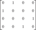
14–15 Sketch the graph for the given adjacency matrix.
- 14.

- 15.
- 16. Complete graph. Show that a graph G with n vertices can have at most n(n − 1)/2 edges, and G has exactly n(n − 1)/2 edges if G is complete, that is, if every pair of vertices of G is joined by an edge. (Recall that loops and multiple edges are excluded.)
- 17. In what case are all the off-diagonal entries of the adjacency matrix of a graph G equal to one?
- 18. Incidence matrix B of a graph. The definition is B = [bjk], where

Find the incidence matrix of the graph in Prob. 8.
- 19. Incidence matrix
 of a digraph. The definition is
  , where
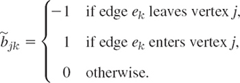
Find the incidence matrix of the digraph in Prob. 11.
- 20. Make the vertex incidence list of the digraph in Prob. 11.
23.2 Shortest Path Problems. Complexity
The rest of this chapter is devoted to the most important classes of problems of combinatorial optimization that can be represented by graphs and digraphs. We selected these problems because of their importance in applications, and present their solutions in algorithmic form. Although basic ideas and algorithms will be explained and illustrated by small graphs, you should keep in mind that real-life problems may often involve many thousands or even millions of vertices and edges. Think of computer networks, telephone networks, electric power grids, worldwide air travel, and companies that have offices and stores in all larger cities. You can also think of other ideas for networks related to the Internet, such as electronic commerce (networks of buyers and sellers of goods over the Internet) and social networks and related websites, such as Facebook. Hence reliable and efficient systematic methods are an absolute necessity—solutions by trial and error would no longer work, even if “nearly optimal” solutions were acceptable.
We begin with shortest path problems, as they arise, for instance, in designing shortest (or least expensive, or fastest) routes for a traveling salesman, for a cargo ship, etc. Let us first explain what we mean by a path.
In a graph G = (V, E) we can walk from a vertex ν1 along some edges to some other vertex νk. Here we can
- make no restrictions, or
- require that each edge of G be traversed at most once, or
- require that each vertex be visited at most once.
In case (A) we call this a walk. Thus a walk from ν1 to νk is of the form
![]()
where some of these edges or vertices may be the same. In case (B), where each edge may occur at most once, we call the walk a trail. Finally, in case (C), where each vertex may occur at most once (and thus each edge automatically occurs at most once), we call the trail a path.
We admit that a walk, trail, or path may end at the vertex it started from, in which case we call it closed; then νk = ν1 in (1).
A closed path is called a cycle. A cycle has at least three edges (because we do not have double edges; see Sec. 23.1). Figure 481 illustrates all these concepts.

Fig. 481. Walk, trail, path, cycle

Shortest Path
To define the concept of a shortest path, we assume that G = (V, E) is a weighted graph, that is, each edge (νi, νj) in G has a given weight or length lij > 0. Then a shortest path ν1 → νk (with fixed ν1 and νk) is a path (1) such that the sum of the lengths of its edges
![]()
(l12 = length of (ν1, ν2) etc.) is minimum (as small as possible among all paths from ν1 to νk). Similarly, a longest path ν1 → νk is one for which that sum is maximum.
Shortest (and longest) path problems are among the most important optimization problems. Here, “length” lij (often also called “cost” or “weight”) can be an actual length measured in miles or travel time or fuel expenses, but it may also be something entirely different.
For instance, the traveling salesman problem requires the determination of a shortest Hamiltonian1 cycle in a graph, that is, a cycle that contains all the vertices of the graph.
In more detail, the traveling salesman problem in its most basic and intuitive form can be stated as follows. You have a salesman who has to drive by car to his customers. He has to drive to n cities. He can start at any city and after completion of the trip he has to return to that city. Furthermore, he can only visit each city once. All the cities are linked by roads to each other, so any city can be visited from any other city directly, that is, if he wants to go from one city to another city, there is only one direct road connecting those two cities. He has to find the optimal route, that is, the route with the shortest total mileage for the overall trip. This is a classic problem in combinatorial optimization and comes up in many different versions and applications. The maximum number of possible paths to be examined in the process of selecting the optimal path for n cities is (n − 1)!/2, because, after you pick the first city, you have n − 1 choices for the second city, n − 2 choices for the third city, etc. You get a total of (n − 1)! (see Sec. 24.4). However, since the mileage does not depend on the direction of the tour (e.g., for n = 4 (four cities 1, 2, 3, 4), the tour 1–2–3–4–1 has the same mileage as 1–4–3–2–1, etc., so that we counted all the tours twice!), the final answer is (n − 1)!/2. Even for a small number of cities, say n = 15, the maximum number of possible paths is very large. Use your calculator or CAS to see for yourself! This means that this is a very difficult problem for larger n and typical of problems in combinatorial optimization, in that you want a discrete solution but where it might become nearly impossible to explicitly search through all the possibilities and therefore some heuristics (rules of thumbs, shortcuts) might be used, and a less than optimal answer suffices.
A variation of the traveling salesman problem is the following. By choosing the “most profitable” route ν1 → νk, a salesman may want to maximize ∑lij, where lij is his expected commission minus his travel expenses for going from town i to town j.
In an investment problem, i may be the day an investment is made, j the day it matures, and lij the resulting profit, and one gets a graph by considering the various possibilities of investing and reinvesting over a given period of time.
Shortest Path If All Edges Have Length l = 1
Obviously, if all edges have length l, then a shortest path ν1 → νk is one that has the smallest number of edges among all paths ν1 → νk in a given graph G. For this problem we discuss a BFS algorithm. BFS stands for Breadth First Search. This means that in each step the algorithm visits all neighboring (all adjacent) vertices of a vertex reached, as opposed to a DFS algorithm (Depth First Search algorithm), which makes a long trail (as in a maze). This widely used BFS algorithm is shown in Table 23.1.
We want to find a shortest path in G from a vertex s (start) to a vertex t (terminal). To guarantee that there is a path from s to t, we make sure that G does not consist of separate portions. Thus we assume that G is connected, that is, for any two vertices ν and w there is a path ν → w in G. (Recall that a vertex ν is called adjacent to a vertex u if there is an edge (u, ν) in G.)
Table 23.1 Moore's2 BFS for Shortest Path (All Lengths One)
Proceedings of the International Symposium for Switching Theory, Part II. pp. 285–292. Cambridge: Harvard University Press, 1959.

EXAMPLE 1 Application of Moore's BFS Algorithm
Find a shortest path s → t in the graph G shown in Fig. 482.
Solution. Figure 482 shows the labels. The blue edges form a shortest path (length 4). There is another shortest path s → t. (Can you find it?) Hence in the program we must introduce a rule that makes backtracking unique because otherwise the computer would not know what to do next if at some step there is a choice (for instance, in Fig. 482 when it got back to the vertex labeled 2). The following rule seems to be natural.
Backtracking rule. Using the numbering of the vertices from 1 to n (not the labeling!), at each step, if a vertex labeled i is reached, take as the next vertex that with the smallest number (not label!) among all the vertices labeled i − 1.

Fig. 482. Example 1, given graph and result of labeling
Complexity of an Algorithm
Complexity of Moore's algorithm. To find the vertices to be labeled 1, we have to scan all edges incident with s. Next, when i = 1, we have to scan all edges incident with vertices labeled 1, etc. Hence each edge is scanned twice. These are 2m operations (m = number of edges of G). This is a function c(m). Whether it is 2m or 5m + 3 or 12m is not so essential; it is essential that c(m) is proportional to m (not m2, for example); it is of the “order” m. We write for any function am + b simply O(m), for any function am2 + bm + d simply O(m2), and so on; here, O suggests order. The underlying idea and practical aspect are as follows.
In judging an algorithm, we are mostly interested in its behavior for very large problems (large m in the present case), since these are going to determine the limits of the applicability of the algorithm. Thus, the essential item is the fastest growing term (am2 in am2 + bm + d, etc.) since it will overwhelm the others when m is large enough. Also, a constant factor in this term is not very essential; for instance, the difference between two algorithms of orders, say, 5m2 and 8m2 is generally not very essential and can be made irrelevant by a modest increase in the speed of computers. However, it does make a great practical difference whether an algorithm is of order m or m2 or of a still higher power mp And the biggest difference occurs between these “polynomial orders” and “exponential orders,” such as 2m.
For instance, on a computer that does 109 operations per second, a problem of size m = 50 will take 0.3 sec with an algorithm that requires m5 operations, but 13 days with an algorithm that requires 2m operations. But this is not our only reason for regarding polynomial orders as good and exponential orders as bad. Another reason is the gain in using a faster computer. For example, let two algorithms be O(m) and 0(m2). Then, since 1000 = 31.62, an increase in speed by a factor 1000 has the effect that per hour we can do problems 1000 and 31.6 times as big, respectively. But since 1000 = 29.97, with an algorithm that is O(2m), all we gain is a relatively modest increase of 10 in problem size because 29.97 · 2m = 2m+9.97.
The symbol O is quite practical and commonly used whenever the order of growth is essential, but not the specific form of a function. Thus if a function g(m) is of the form
![]()
we say that g(m) is of the order h(m) and write
![]()
For instance,
![]()
We want an algorithm ![]() to be “efficient,” that is, “good” with respect to
to be “efficient,” that is, “good” with respect to
- Time (number c
 (m) of computer operations), or
 - Space (storage needed in the internal memory)
or both. Here c![]() suggests “complexity” of
suggests “complexity” of ![]() . Two popular choices for c
. Two popular choices for c![]() are
are
(Worst case) c![]() (m) = longest time
(m) = longest time ![]() takes for a problem of size m,
takes for a problem of size m,
Average case) c![]() (m) = average time
(m) = average time ![]() takes for a problem of size m.
takes for a problem of size m.
In problems on graphs, the “size” will often be m (number of edges) or n (number of vertices). For Moore's algorithm, c![]() (m) = 2m in both cases. Hence the complexity of Moore's algorithm is of order O(m).
(m) = 2m in both cases. Hence the complexity of Moore's algorithm is of order O(m).
For a “good” algorithm ![]() , we want that c
, we want that c![]() (m) does not grow too fast. Accordingly, we call
(m) does not grow too fast. Accordingly, we call ![]() efficient if c
efficient if c![]() (m) = O(mk) for some integer k
(m) = O(mk) for some integer k ![]() 0; that is, c
0; that is, c![]() may contain only powers of m (or functions that grow even more slowly, such as ln m), but no exponential functions. Furthermore, we call
may contain only powers of m (or functions that grow even more slowly, such as ln m), but no exponential functions. Furthermore, we call ![]() polynomially bounded if
polynomially bounded if ![]() is efficient when we choose the “worst case” c
is efficient when we choose the “worst case” c![]() (m). These conventional concepts have intuitive appeal, as our discussion shows.
(m). These conventional concepts have intuitive appeal, as our discussion shows.
Complexity should be investigated for every algorithm, so that one can also compare different algorithms for the same task. This may often exceed the level in this chapter; accordingly, we shall confine ourselves to a few occasional comments in this direction.
SHORTEST PATHS, MOORE'S BFS
(All edges length one)
1–4 Find a shortest path p: s → t and its length by Moore's algorithm. Sketch the graph with the labels and indicate P by heavier lines as in Fig. 482.


- Moore's algorithm. Show that if vertex ν has label λ(ν) = k, then there is a path s → ν of length k.
- Maximum length. What is the maximum number of edges that a shortest path between any two vertices in a graph with n vertices can have? Give a reason. In a complete graph with all edges of length 1?
- Nonuniqueness. Find another shortest path from s to t in Example 1 of the text.
- Moore's algorithm. Call the length of a shortest path s → ν the distance of ν from s. Show that if ν has distance l, it has label λ(ν) = l.
- CAS PROBLEM. Moore's Algorithm. Write a computer program for the algorithm in Table 23.1. Test the program with the graph in Example 1. Apply it to Probs. 1–3 and to some graphs of your own choice.
10–12 HAMILTONIAN CYCLE
- 10. Find and sketch a Hamiltonian cycle in the graph of a dodecahedron, which has 12 pentagonal faces and 20 vertices (Fig. 483). This is a problem Hamilton himself considered.

- 11. Find and sketch a Hamiltonian cycle in Prob. 1.
- 12. Does the graph in Prob. 4 have a Hamiltonian cycle?
13–14 POSTMAN PROBLEM
- 13. The postman problem is the problem of finding a closed walk W: s → s (s the post office) in a graph G with edges (i, j) of length lij > 0 such that every edge of G is traversed at least once and the length of W is minimum. Find a solution for the graph in Fig. 484 by inspection. (The problem is also called the Chinese postman problem since it was published in the journal Chinese Mathematics 1 (1962), 273–277.)

- 14. Show that the length of a shortest postman trail is the same for every starting vertex.
15–17 EULER GRAPHS
- 15. An Euler graphG is a graph that has a closed Euler trail. An Euler trail is a trail that contains every edge of G exactly once. Which subgraph with four edges of the graph in Example 1, Sec. 23.1, is an Euler graph?
- 16. Find four different closed Euler trails in Fig. 485.

- 17. Is the graph in Fig. 484 an Euler graph. Give reason.
18–20 ORDER
- 18. Show that O(m3) = O(m3) = O(m3) and kO(mp) = O(mp).
- 19. show that
 .
. - 20. If we switch from one computer to another that is 100 times as fast, what is our gain in problem size per hour in the use of an algorithm that is O(m), O(m2), O(m5), O(em)?
23.3 Bellman's Principle. Dijkstra's Algorithm
We continue our discussion of the shortest path problem in a graph G. The last section concerned the special case that all edges had length 1. But in most applications the edges (i, j) will have any lengths lij > 0, and we now turn to this general case, which is of greater practical importance. We write lij = ∞ for any edge (i, j) that does not exist in G (setting ∞ + a = ∞ for any number a, as usual).
We consider the problem of finding shortest paths from a given vertex, denoted by 1 and called the origin, to all other vertices 2, 3, … n of G. We let Lj denote the length of a shortest path Pj: 1 → j in G.
THEOREM 1 Bellman's Minimality Principle or Optimality Principle3
If Pj: 1 → j is a shortest path from1 to j in G and (i, j) is the last edge of Pj (Fig. 486), then Pi: 1 → i [obtained by dropping (i, j) from Pj] is a shortest path 1: → i.
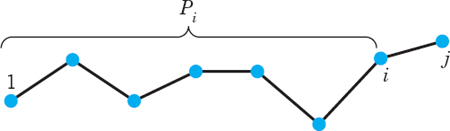
Fig. 486. Paths P and Pi in Bellman's minimality principle
PROOF
Suppose that the conclusion is false. Then there is a path ![]() that is shorter than Pi. Hence, if we now add (i, j) to
that is shorter than Pi. Hence, if we now add (i, j) to ![]() , we get a path 1 → j that is shorter than Pj. This contradicts our assumption that Pj is shortest.
, we get a path 1 → j that is shorter than Pj. This contradicts our assumption that Pj is shortest.
From Bellman's principle we can derive basic equations as follows. For fixed j we may obtain various paths 1 → j by taking shortest paths Pi for various i for which there is in G an edge (i, j), and add (i, j) to the corresponding Pi. These paths obviously have lengths Li + lij (Li = length of Pi). We can now take the minimum over i, that is, pick an i for which Li + lij is smallest. By the Bellman principle, this gives a shortest path 1 → j. It has the length

These are the Bellman equations. Since lii = 0 by definition, instead of mini≠j we can simply write mini. These equations suggest the idea of one of the best-known algorithms for the shortest path problem, as follows.
Dijkstra's Algorithm for Shortest Paths
Dijkstra's4algorithm is shown in Table 23.2, where a connected graphG is a graph in which, for any two vertices ν and w in G, there is a path ν → ω. The algorithm is a labeling procedure. At each stage of the computation, each vertex ν gets a label, either
![]()
or
![]()
We denote by ![]()
![]() and
and ![]()
![]() the sets of vertices with a permanent label and with a temporary label, respectively. The algorithm has an initial step in which vertex 1 gets the permanent label L1 = 0 and the other vertices get temporary labels, and then the algorithm alternates between Steps 2 and 3. In Step 2 the idea is to pick k “minimally.” In Step 3 the idea is that the upper bounds will in general improve (decrease) and must be updated accordingly. Namely, the new temporary label
the sets of vertices with a permanent label and with a temporary label, respectively. The algorithm has an initial step in which vertex 1 gets the permanent label L1 = 0 and the other vertices get temporary labels, and then the algorithm alternates between Steps 2 and 3. In Step 2 the idea is to pick k “minimally.” In Step 3 the idea is that the upper bounds will in general improve (decrease) and must be updated accordingly. Namely, the new temporary label ![]() of vertex j will be the old one if there is no improvement or it will be Lk + lkj if there is.
of vertex j will be the old one if there is no improvement or it will be Lk + lkj if there is.
Table 23.2 Dijkstra's Algorithm for Shortest Paths

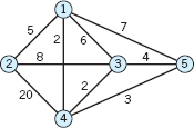
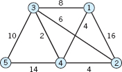
EXAMPLE 1 Application of Dijkstra's Algorithm
Applying Dijkstra's algorithm to the graph in Fig. 487a, find shortest paths from vertex 1 to vertices 2, 3, 4.
Solution. We list the steps and computations.

Figure 487b shows the resulting shortest paths, of lengths L2 = 6, L3 = 5, L4 = 7.
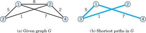
Fig. 487. Example 1
Complexity. Dijkstra's algorithm is O(n2).
PROOF
Step 2 requires comparison of elements, first n − 2, the next time n− 3, etc., a total of (n − 2)(n − 1)/2. Step 3 requires the same number of comparisons, a total of (n − 2)(n − 1)/2, as well as additions, first n − 2, the next time n − 3, etc., again a total of (n − 2)(n −)/2. Hence the total number of operations is 3(n − 2)(n − 1)/2 = O(n2).
- The net of roads in Fig. 488 connecting four villages is to be reduced to minimum length, but so that one can still reach every village from every other village. Which of the roads should be retained? Find the solution (a) by inspection, (b) by Dijkstra's algorithm.

- Show that in Dijkstra's algorithm, for Lk there is a path P: 1 → k of length Lk.
- Show that in Dijkstra's algorithm, at each instant the demand on storage is light (data for fewer than n edges).
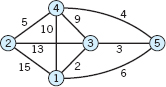
4–9 DIJKSTRA'S ALGORITHM
For each graph find the shortest paths.


23.4 Shortest Spanning Trees: Greedy Algorithm
So far we have discussed shortest path problems. We now turn to a particularly important kind of graph, called a tree, along with related optimization problems that arise quite often in practice.
By definition, a tree T is a graph that is connected and has no cycles. “Connected” was defined in Sec. 23.3; it means that there is a path from any vertex in T to any other vertex in T. A cycle is a path s → t of at least three edges that is closed (t = s); see also Sec. 23.2. Figure 489a shows an example.
CAUTION! The terminology varies; cycles are sometimes also called circuits.
A spanning tree T in a given connected graph G = (V, E) is a tree containing all the n vertices of G. See Fig. 489b. Such a tree has n − 1 edges. (Proof?)
A shortest spanning tree T in a connected graph G (whose edges (i, j) have lengths lij > 0) is a spanning tree for which ∑lij (sum over all edges of T) is minimum compared to ∑lij for any other spanning tree in G.

Fig. 489. Example of (a) a cycle, (b) a spanning tree in a graph
Trees are among the most important types of graphs, and they occur in various applications. Familiar examples are family trees and organization charts. Trees can be used to exhibit, organize, or analyze electrical networks, producer–consumer and other business relations, information in database systems, syntactic structure of computer programs, etc. We mention a few specific applications that need no lengthy additional explanations.
The set of shortest paths from vertex 1 to the vertices 2, …, n in the last section forms a spanning tree.
Railway lines connecting a number of cities (the vertices) can be set up in the form of a spanning tree, the “length” of a line (edge) being the construction cost, and one wants to minimize the total construction cost. Similarly for bus lines, where “length” may be the average annual operating cost. Or for steamship lines (freight lines), where “length” may be profit and the goal is the maximization of total profit. Or in a network of telephone lines between some cities, a shortest spanning tree may simply represent a selection of lines that connect all the cities at minimal cost. In addition to these examples we could mention others from distribution networks, and so on.
We shall now discuss a simple algorithm for the problem of finding a shortest spanning tree. This algorithm (Table 23.3) is particularly suitable for sparse graphs (graphs with very few edges; see Sec. 23.1).
Table 23.3 Kruskal's5Greedy Algorithm for Shortest Spanning Trees
Proceedings of the American Mathematical Society 7 (1956), 48–50.

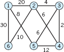
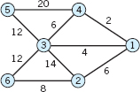
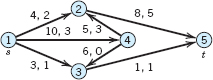
EXAMPLE 1 Application of Kruskal's Algorithm
Using Kruskal's algorithm, we shall determine a shortest spanning tree in the graph in Fig. 490.

Fig. 490. Graph in Example 1
Table 23.4 Solution in Example 1

Solution. See Table 23.4. In some of the intermediate stages the edges chosen form a disconnected graph (see Fig. 491); this is typical. We stop after n − 1 = 5 choices since a spanning tree has n − 1 edges. In our problem the edges chosen are in the upper part of the list. This is typical of problems of any size; in general, edges farther down in the list have a smaller chance of being chosen.
The efficiency of Kruskal's method is greatly increased by double labeling of vertices.
Double Labeling of Vertices. Each vertex i carries a double label (ri, pi), where

This simplifies rejecting.
Rejecting. If (i, j) is next in the list to be considered, reject (i, j) if ri = rj (that is, i and j are in the same subtree, so that they are already joined by edges and (i, j) would thus create a cycle). If ri ≠ rj, include (i, j) in T.
If there are several choices for ri, choose the smallest. If subtrees merge (become a single tree), retain the smallest root as the root of the new subtree.
For Example 1 the double-label list is shown in Table 23.5. In storing it, at each instant one may retain only the latest double label. We show all double labels in order to exhibit the process in all its stages. Labels that remain unchanged are not listed again. Underscored are the two 1’s that are the common root of vertices 2 and 3, the reason for rejecting the edge (2, 3). By reading for each vertex the latest label we can read from this list that 1 is the vertex we have chosen as a root and the tree is as shown in the last part of Fig. 491.

Fig. 491. Choice process in Example 1
Table 23.5 List of Double Labels in Example 1

This is made possible by the predecessor label that each vertex carries. Also, for accepting or rejecting an edge we have to make only one comparison (the roots of the two endpoints of the edge).
Ordering is the more expensive part of the algorithm. It is a standard process in data processing for which various methods have been suggested (see Sorting in Ref. [E25] listed in App. 1). For a complete list of m edges, an algorithm would be O(m log2 m), but since the n − 1 edges of the tree are most likely to be found earlier, by inspecting the q (< m) topmost edges, for such a list of q edges one would have O(q log2 m).
1–6 KRUSKAL'S GREEDY ALGORITHM
Find a shortest spanning tree by Kruskal's algorithm. Sketch it.


- CAS PROBLEM. Kruskal's Algorithm. Write a corresponding program. (Sorting is discussed in Ref. [E25] listed in App. 1.)
- To get a minimum spanning tree, instead of adding shortest edges, one could think of deleting longest edges. For what graphs would this be feasible? Describe an algorithm for this.
- Apply the method suggested in Prob. 8 to the graph in Example 1. Do you get the same tree?
- Design an algorithm for obtaining longest spanning trees.
- Apply the algorithm in Prob. 10 to the graph in Example 1. Compare with the result in Example 1.
- Forest. A (not necessarily connected) graph without cycles is called a forest. Give typical examples of applications in which graphs occur that are forests or trees.
- Air cargo. Find a shortest spanning tree in the complete graph of all possible 15 connections between the six cities given (distances by airplane, in miles, rounded). Can you think of a practical application of the result?

14–20 GENERAL PROPERTIES OF TREES
Prove the following. Hint. Use Prob. 14 in proving 15 and 18; use Probs. 16 and 18 in proving 20.
- 14. Uniqueness. The path connecting any two vertices u and ν in a tree is unique.
- 15. If in a graph any two vertices are connected by a unique path, the graph is a tree.
- 16. If a graph has no cycles, it must have at least 2 vertices of degree 1 (definition in Sec. 23.1).
- 17. A tree with exactly two vertices of degree 1 must be a path.
- 18. A tree with n vertices has n − 1 edges. (Proof by induction.)
- 19. If two vertices in a tree are joined by a new edge, a cycle is formed.
- 20. A graph with n vertices is a tree if and only if it has n − 1 edges and has no cycles.
23.5 Shortest Spanning Trees:
Prim's Algorithm
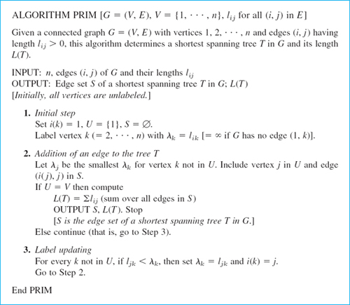
Prim's6 algorithm, shown in Table 23.6, is another popular algorithm for the shortest spanning tree problem (see Sec. 23.4). This algorithm avoids ordering edges and gives a tree T at each stage, a property that Kruskal's algorithm in the last section did not have (look back at Fig. 491 if you did not notice it).
In Prim's algorithm, starting from any single vertex, which we call 1, we “grow” the tree T by adding edges to it, one at a time, according to some rule (in Table 23.6) until T finally becomes a spanning tree, which is shortest.
We denote by U the set of vertices of the growing tree T and by S the set of its edges. Thus, initially U = { 1 } and S = Ø; at the end U = V, the vertex set of the given graph G = (V, E), whose edges (i, j) have length lij > 0, as before.
Thus at the beginning (Step 1) the labels
![]()
are the lengths of the edges connecting them to vertex 1 (or ∞ if there is no such edge in G). And we pick (Step 2) the shortest of these as the first edge of the growing tree T and include its other end j in U (choosing the smallest j if there are several, to make the process unique). Updating labels in Step 3 (at this stage and at any later stage) concerns each vertex k not yet in U. Vertex k has label λk = li(k),k from before. If ljk < λk, this means that k is closer to the new member j just included in U than k is to its old “closest neighbor” i(k) in U. Then we update the label of k, replacing λk = li(k),k by λk = ljk and setting i(k) = j. If, however, ljk ![]() λk (the old label of k), we don't touch the old label. Thus the label λk always identifies the closest neighbor of k in U, and this is updated in Step 3 as U and the tree T grow. From the final labels we can backtrack the final tree, and from their numeric values we compute the total length (sum of the lengths of the edges) of this tree.
λk (the old label of k), we don't touch the old label. Thus the label λk always identifies the closest neighbor of k in U, and this is updated in Step 3 as U and the tree T grow. From the final labels we can backtrack the final tree, and from their numeric values we compute the total length (sum of the lengths of the edges) of this tree.
Prim's algorithm is useful for computer network design, cable, distribution networks, and transportation networks.
Table 23.6 Prim's Algorithm for Shortest Spanning Trees
Bell System Technical Journal 36 (1957), 1389–1401.
For an improved version of the algorithm, see Cheriton and Tarjan, SIAM Journal on Computation 5 (1976), 724–742.
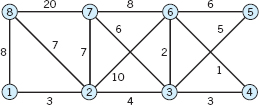
EXAMPLE 1 Application of Prim's Algorithm

Fig. 492. Graph in Example 1
Find a shortest spanning tree in the graph in Fig. 492 (which is the same as in Example 1, Sec. 23.4, so that we can compare).
Solution. The steps are as follows.
- 1. i(k) = 1, U = {1}, S = Ø, initial labels see Table 23.7.
- 2. λ2 = l12 = 2 is smallest, U = {1, 2}, S = {(1, 2)}.
- 3. Update labels as shown in Table 23.7, column (I).
- 2. λ3 = l13 = 4 is smallest, U = {1, 2, 3}, S = {(1, 2), (1, 3)}.
- 3. Update labels as shown in Table 23.7, column (II).
- 2. λ6 = l36 = 1 is smallest, U = {1, 2, 3, 6}, S = {(1, 2), (1, 3), (3, 6)}.
- 3. Update labels as shown in Table 23.7, column (III).
- 2. λ4 = l34 = 8 is smallest, U = {1, 2, 3, 4, 6}, S = {(1, 2), (1, 3), (3, 4), (3, 6)}.
- 3. Update labels as shown in Table 23.7, column (IV).
- 2. λ5 = l45 = 6 is smallest, U =V, S = (1, 2), (1, 3), (3, 4), (3, 6), (4, 5). Stop.
The tree is the same as in Example 1, Sec. 23.4. Its length is 21. You will find it interesting to compare the growth process of the present tree with that in Sec. 23.4.
Table 23.7 Labeling of Vertices in Example 1

SHORTEST SPANNING TREES. PRIM'S ALGORITHM
- When will S = E at the end in Prim's algorithm?
- Complexity. Show that Prim's algorithm has complexity O(n2).
- What is the result of applying Prim's algorithm to a graph that is not connected?
- If for a complete graph (or one with very few edges missing), our data is an n × n distance table (as in Prob. 13, Sec. 23.4), show that the present algorithm [which is O(n2)] cannot easily be replaced by an algorithm of order less than O(n2).
- How does Prim's algorithm prevent the generation of cycles as you grow T?
6–13 Find a shortest spanning tree by Prim's algorithm.
- 6.
- 7.
- 8.
- 9.
- 10. For the graph in Prob. 6, Sec. 23.4.
- 11. For the graph in Prob. 4, Sec. 23.4.
- 12. For the graph in Prob. 2, Sec. 23.4.
- 13. CAS PROBLEM. Prim's Algorithm. Write a program and apply it to Probs. 6–9.
- 14. TEAM PROJECT. Center of a Graph and Related Concepts. (a) Distance, Eccentricity. Call the length of a shortest path u → ν in a graph G = (V, E) the distance d(u, ν)from u to ν. For fixed u, call the greatest d(u, ν) as ν ranges over V the eccentricity ∈(u) of u. Find the eccentricity of vertices 1, 2, 3 in the graph in Prob. 7.
(b) Diameter, Radius, Center. The diameter d(G) of a graph G = (V, E) is the maximum of d(u, ν) as u and ν vary over V, and the radius r(G) is the smallest eccentricity ∈(ν) of the vertices ν. A vertex ν with ∈(ν) = r(G) is called a central vertex. The set of all central vertices is called the center of G. Find d(G), r(G), and the center of the graph in Prob. 7.
(c) What are the diameter, radius, and center of the spanning tree in Example 1 of the text?
(d) Explain how the idea of a center can be used in setting up an emergency service facility on a transportation network. In setting up a fire station, a shopping center. How would you generalize the concepts in the case of two or more such facilities?
(e) Show that a tree T whose edges all have length 1 has center consisting of either one vertex or two adjacent vertices.
(f) Set up an algorithm of complexity O(n) for finding the center of a tree T.
23.6 Flows in Networks
After shortest path problems and problems for trees, as a third large area in combinatorial optimization we discuss flow problems in networks (electrical, water, communication, traffic, business connections, etc.), turning from graphs to digraphs (directed graphs; see Sec. 23.1).
By definition, a network is a digraph G = (V, E) in which each edge (i, j) has assigned to it a capacity cij > 0 [= maximum possible flow along (i, j)], and at one vertex, s, called the source, a flow is produced that flows along the edges of the digraph G to another vertex, t, called the target or sink, where the flow disappears.
In applications, this may be the flow of electricity in wires, of water in pipes, of cars on roads, of people in a public transportation system, of goods from a producer to consumers, of e-mail from senders to recipients over the Internet, and so on.
We denote the flow along a (directed!) edge (i, j) by fij and impose two conditions:
1. For each edge (i, j) in G the flow does not exceed the capacity cij,
![]()
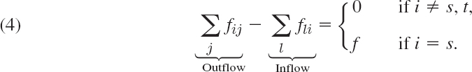
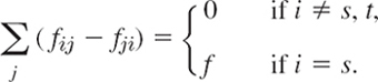
2. For each vertex i, not s or t,
![]()

where f is the total flow (and at s the inflow is zero, whereas at t the outflow is zero). Figure 493 illustrates the notation (for some hypothetical figures).
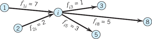
Fig. 493. Notation in (2): inflow and outflow for a vertex i (not s or t)
Paths
By a path ν1 → νk from a vertex ν1 to a vertex νk in a digraph G we mean a sequence of edges
![]()
regardless of their directions in G, that forms a path as in a graph (see Sec. 23.2). Hence when we travel along this path from ν1 to νk we may traverse some edge in its given direction—then we call it a forward edge of our path—or opposite to its given direction—then we call it a backward edge of our path. In other words, our path consists of one-way streets, and forward edges (backward edges) are those that we travel in the right direction (in the wrong direction). Figure 494 shows a forward edge (u, v) and a backward edge (w, v) of a path ν1 → νk.
CAUTION! Each edge in a network has a given direction, which we cannot change. Accordingly, if (u, v) is a forward edge in a path ν1 → νk, then (u, v) can become a backward edge only in another path x1 → xj in which it is an edge and is traversed in the opposite direction as one goes from x1 to xj; see Fig. 495. Keep this in mind, to avoid misunderstandings.

Fig. 494. Forward edge (u, v) and backward edge (w, v) of a path v1 → vk
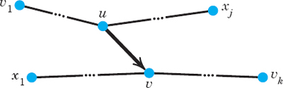
Fig. 495. Edge (u, v) as forward edge in the path v1 → vk and as backward edge in the path x1 → xj
Flow Augmenting Paths
Our goal will be to maximize the flow from the source s to the target t of a given network. We shall do this by developing methods for increasing an existing flow (including the special case in which the latter is zero). The idea then is to find a path P: s → t all of whose edges are not fully used, so that we can push additional flow through P. This suggests the following concept.
DEFINITION Flow Augmenting Path
A flow augmenting path in a network with a given flow fij on each edge (i, j) is a path P: s → t such that
- no forward edge is used to capacity; thus fij < cij for these;
- no backward edge has flow 0; thus fij > 0 for these.
EXAMPLE 1 Flow Augmenting Paths
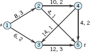
Find flow augmenting paths in the network in Fig. 496, where the first number is the capacity and the second number a given flow.

Fig. 496. Network in Example 1 First number = Capacity, Second number = Given flow
Solution. In practical problems, networks are large and one needs a systematic method for augmenting flows, which we discuss in the next section. In our small network, which should help to illustrate and clarify the concepts and ideas, we can find flow augmenting paths by inspection and augment the existing flow f = 9 in Fig. 496. (The outflow from s is 5 + 4 = 9, which equals the inflow 6 + 3 into t.)
We use the notation
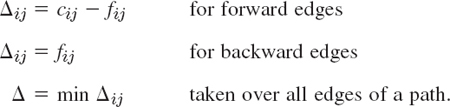
From Fig. 496 we see that a flow augmenting path p1: s → t is p1: 1 − 2 − 3 − 6 (Fig. 497), with Δ12 = 20 − 5 = 15, etc., and Δ = 3. Hence we can use P1 to increase the given flow 9 to f = 9 + 3 = 12. All three edges of p1 are forward edges. We augment the flow by 3. Then the flow in each of the edges of p1 is increased by 3, so that we now have f12 = 8 (instead of 5), f23 = 11 (instead of 8), and f36 = 9 (instead of 6). Edge (2, 3) is now used to capacity. The flow in the other edges remains as before.
We shall now try to increase the flow in this network in Fig. 496 beyond f = 12.
There is another flow augmenting path p2: s → t, namely, p2: 1 − 4 − 5 − 3 − 6 (Fig. 497). It shows how a backward edge comes in and how it is handled. Edge (3, 5) is a backward edge. It has flow 2, so that Δ36 = 2. We compute Δ14 = 10 − 4 = 6, etc. (Fig. 497) and Δ = 2. Hence we can use p2 for another augmentation to get f = 12 + 2 = 14. The new flow is shown in Fig. 498. No further augmentation is possible. We shall confirm later that f = 14 is maximum.

Fig. 497. Flow augmenting paths in Example 1
Cut Sets
A cut set is a set of edges in a network. The underlying idea is simple and natural. If we want to find out what is flowing from s to t in a network, we may cut the network somewhere between s and t (Fig. 498 shows an example) and see what is flowing in the edges hit by the cut, because any flow from s to t must sometimes pass through some of these edges. These form what is called a cut set. [In Fig. 498, the cut set consists of the edges (2, 3), (5, 2), (4, 5).] We denote this cut set by (S, T). Here S is the set of vertices on that side of the cut on which s lies (S = {s, 2, 4} for the cut in Fig. 498) and T is the set of the other vertices (T = {3, 5, t} in Fig. 498). We say that a cut partitions the vertex set V into two parts S and T. Obviously, the corresponding cut set (S, T) consists of all the edges in the network with one end in S and the other end in T.

Fig. 498. Maximum flow in Example 1
By definition, the capacity cap (S, T) of a cut set (S, T) is the sum of the capacities of all forward edges in (S, T) (forward edges only!), that is, the edges that are directed from S to T,
![]()
Thus, cap (S, T) = 11 + 7 = 18 in Fig. 498.
Explanation. This can be seen as follows. Look at Fig. 498. Recall that for each edge in that figure, the first number denotes capacity and the second number flow. Intuitively, you can think of the edges as roads, where the capacity of the road is how many cars can actually be on the road, and the flow denotes how many cars actually are on the road. To compute capacity cap (S, T) we are only looking at the first number on the edges. Take a look and see that the cut physically cuts three edges, that is, (2, 3), (4, 5), and (5, 2). The cut concerns only forward edges that are being cut, so it concerns edges (2, 3) and (4, 5) (and does not include edge (5, 2) which is also being cut, but since it goes backwards, it does not count). Hence (2, 3) contributes 11 and (4, 5) contributes 7 to the capacity cap (S, T), for a total of 18 in Fig. 498. Hence (S, T) = 18.
The other edges (directed from T to S) are called backward edges of the cut set (S, T), and by the net flow through a cut set we mean the sum of the flows in the forward edges minus the sum of the flows in the backward edges of the cut set.
CAUTION! Distinguish well between forward and backward edges in a cut set and in a path: (5, 2) in Fig. 498 is a backward edge for the cut shown but a forward edge in the path 1 − 4 − 5 − 2 − 3 − 6.
For the cut in Fig. 498 the net flow is 11 + 6 − 3 = 14. For the same cut in Fig. 496 (not indicated there), the net flow is 8 + 4 − 3 = 9. In both cases it equals the flow f. We claim that this is not just by chance, but cuts do serve the purpose for which we have introduced them:
THEOREM 1 Net Flow in Cut Sets
Any given flow in a network G is the net flow through any cut set (S, T) of G.
PROOF
By Kirchhoff's law (2), multiplied by −1, at a vertex i we have
Here we can sum over j and l from 1 to n (= number of vertices) by putting fij = 0 for j = i and also for edges without flow or nonexisting edges; hence we can write the two sums as one,
We now sum over all i in S. Since s is in S, this sum equals f:

We claim that in this sum, only the edges belonging to the cut set contribute. Indeed, edges with both ends in T cannot contribute, since we sum only over i in S; but edges (i, j) with both ends in S contribute +fij at one end and −fij at the other, a total contribution of 0. Hence the left side of (5) equals the net flow through the cut set. By (5), this is equal to the flow f and proves the theorem.
This theorem has the following consequence, which we shall also need later in this section.
THEOREM 2 Upper Bound for Flows
A flow f in a network G cannot exceed the capacity of any cut set (S, T) in G.
PROOF
By Theorem 1 the flow f equals the net flow through the cut set, f = f1 − f2, where f1 is the sum of the flows through the forward edges and f2 (![]() 0) is the sum of the flows through the backward edges of the cut set. Thus f
0) is the sum of the flows through the backward edges of the cut set. Thus f ![]() f1. Now f1 cannot exceed the sum of the capacities of the forward edges; but this sum equals the capacity of the cut set, by definition. Together, f
f1. Now f1 cannot exceed the sum of the capacities of the forward edges; but this sum equals the capacity of the cut set, by definition. Together, f ![]() cap (S, T), as asserted.
cap (S, T), as asserted.
Cut sets will now bring out the full importance of augmenting paths:
THEOREM 3 Main Theorem. Augmenting Path Theorem for Flows
A flow from s to t in a network G is maximum if and only if there does not exist a flow augmenting path s → t in G.
PROOF
(a) If there is a flow augmenting path P: s → t, we can use it to push through it an additional flow. Hence the given flow cannot be maximum.
(b) On the other hand, suppose that there is no flow augmenting path s → t in G. Let S0 be the set of all vertices i (including s) such that there is a flow augmenting path s → i, and let T0 be the set of the other vertices in G. Consider any edge (i, j) with i in S0 and j in T0. Then we have a flow augmenting path s → i since i is in S0, but s → i → j is not flow augmenting because j is not in S0. Hence we must have

Otherwise we could use (i, j) to get a flow augmenting path s → i → j. Now (S0, T0) defines a cut set (since t is in T0; why?). Since by (6), forward edges are used to capacity and backward edges carry no flow, the net flow through the cut set (S0, T0) equals the sum of the capacities of the forward edges, which is cap (S0, T0) by definition. This net flow equals the given flow f by Theorem 1. Thus f = cap (S0, T0). We also have f ![]() cap (S0, T0) by Theorem 2. Hence f must be maximum since we have reached equality.
cap (S0, T0) by Theorem 2. Hence f must be maximum since we have reached equality.
The end of this proof yields another basic result (by Ford and Fulkerson, Canadian Journal of Mathematics 8 (1956), 399–404), namely, the so-called
THEOREM 4 Max-Flow Min-Cut Theorem
The maximum flow in any network G equals the capacity of a“minimum cut set” (= a cut set of minimum capacity) in G.
PROOF
We have just seen that f = cap (S0, T0) for a maximum flow f and a suitable cut set (S0, T0). Now by Theorem 2 we also have f ![]() cap (S, T) for this f and any cut set (S, T) in G. Together, cap (S0, T0)
cap (S, T) for this f and any cut set (S, T) in G. Together, cap (S0, T0) ![]() cap (S, T). Hence (S0, T0) is a minimum cut set.
cap (S, T). Hence (S0, T0) is a minimum cut set.
The existence of a maximum flow in this theorem follows for rational capacities from the algorithm in the next section and for arbitrary capacities from the Edmonds–Karp BFS also in that section.
The two basic tools in connection with networks are flow augmenting paths and cut sets. In the next section we show how flow augmenting paths can be used in an algorithm for maximum flows.
1–6 CUT SETS, CAPACITY
Find T and cap (S, T) for:
- Fig. 498, S = {1, 2, 4, 5}
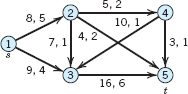
- Fig. 499, S = {1, 2, 3}
- Fig. 498, S = {1, 2, 3}
- Fig. 499, S = {1, 2,}
- Fig. 499, S = {1, 2, 4, 5}
- Fig. 498, S = {1, 3, 5}

7–8 MINIMUM CUT SET
Find a minimum cut set and its capacity for the network:
- 7. In Fig. 499
- 8. In Fig. 496. Verify that its capacity equals the maximum flow.
- 9. Why are backward edges not considered in the definition of the capacity of a cut set?
- 10. Incremental network. Sketch the network in Fig. 499, and on each edge (i, j) write cij − fij and fij. Do you recognize that from this “incremental network” one can more easily see flow augmenting paths?
- 11. Omission of edges. Which edges could be omitted from the network in Fig. 499 without decreasing the maximum flow?
12–15 FLOW AUGMENTING PATHS
Find flow augmenting paths:
- 12.

- 13.
- 14.
- 15.
16–19 MAXIMUM FLOW
Find the maximum flow by inspection:
- 16. In Prob. 13
- 17.

- 18. In Prob. 12
- 19.

- 20. Find another maximum flow f = 15 in Prob. 19.
23.7 Maximum Flow: Ford–Fulkerson Algorithm
Flow augmenting paths, as discussed in the last section, are used as the basic tool in the Ford–Fulkerson7 algorithm in Table 23.8 in which a given flow (for instance, zero flow in all edges) is increased until it is maximum. The algorithm accomplishes the increase by a stepwise construction of flow augmenting paths, one at a time, until no further such paths can be constructed, which happens precisely when the flow is maximum.
In Step 1, an initial flow may be given. In Step 3, a vertex j can be labeled if there is an edge (i, j) with i labeled and
![]()
or if there is an edge (j, i) with i labeled and
![]()
To scan a labeled vertex i means to label every unlabeled vertex j adjacent to i that can be labeled. Before scanning a labeled vertex i, scan all the vertices that got labeled before i. This BFS (Breadth First Search) strategy was suggested by Edmonds and Karp in 1972 (Journal of the Association for Computing Machinery 19, 248–64). It has the effect that one gets shortest possible augmenting paths.
Table 23.8 Ford–Fulkerson Algorithm for Maximum Flow
Canadian Journal of Mathematics 9 (1957), 210–218


EXAMPLE 1 Ford–Fulkerson Algorithm
Applying the Ford–Fulkerson algorithm, determine the maximum flow for the network in Fig. 500 (which is the same as that in Example 1, Sec. 23.6, so that we can compare).
Solution. The algorithm proceeds as follows.
- 1. An initial flow f = 9 is given.
- 2. Label s (= 1) by Ø. Mark 2, 3, 4, 5, 6 “unlabeled.”

Fig. 500. Network in Example 1 with capacities (first numbers) and given flow
- 3. Scan 1.
Compute Δ12 = 20 − 5 = 15 = Δ2. Label 2 by (1+, 15).
Compute Δ14 = 10 − 4 = 6 = Δ4. Label 4 by (1+, 6).
- 4. Scan 2.
Compute Δ23 = 11 − 8 = 3, Δ3 = min (Δ2, 3) = 3. Label 3 by (2+, 3).
Compute Δ5 = min (Δ2, 3) = 3. Label 5 by (2−, 3).
Scan 3.
Compute Δ36 = 13 − 6 = 7, Δ6 = Δt = min (Δ3, 7) = 3. Label 6 by (3+, 3).
- 5. p: 1 − 2 − 3 − 6 (= t) is a flow augmenting path.
- 6. Δt = 3. Augmentation gives f12 = 8, f23 = 11, f36 = 9, other fij unchanged. Augmented flow f = 9 + 3 = 12.
- 7. Remove labels on vertices 2, …, 6. Go to Step 3.
- 3. Scan 1.
Compute Δ12 = 20 − 8 = 12 = Δ2. Label 2 by (1+, 12).
Compute Δ14 = 10 − 4 = 6 = Δ4. Label 4 by (1+, 6).
- 4. Scan 2.
Compute Δ5 = min (Δ2, 3) = 3. Label 5 by (2−, 3).
Scan 4. [No vertex left for labeling.]
Scan 5.
Compute Δ3 = min (Δ5, 2) = 2. Label 3 by (5−, 2).
Scan 3.
Compute Δ36 = 13 − 9 = 4, Δ6 = min (Δ3, 4) = 2. Label 6 by (3+, 2).
- 5. p: 1 − 2 − 5 − 3 − 6 (= t) is a flow augmenting path.
- 6. Δt = 2. Augmentation gives f12 = 10, f32 = 1, f35 = 0, f36 = 11, other fij unchanged. Augmented flow f = 12 + 2 = 14.
- 7. Remove labels on vertices 2, …, 6. Go to Step 3.
One can now scan 1 and then scan 2, as before, but in scanning 4 and then 5 one finds that no vertex is left for labeling. Thus one can no longer reach t. Hence the flow obtained (Fig. 501) is maximum, in agreement with our result in the last section.

Fig. 501. Maximum flow in Example 1
- Do the computations indicated near the end of Example 1 in detail.
- Solve Example 1 by Ford–Fulkerson with initial flow 0. Is it more work than in Example 1?
- Which are the “bottleneck” edges by which the flow in Example 1 is actually limited? Hence which capacities could be decreased without decreasing the maximum flow?
- What is the (simple) reason that Kirchhoff's law is preserved in augmenting a flow by the use of a flow augmenting path?
- How does Ford–Fulkerson prevent the formation of cycles?
6–9 MAXIMUM FLOW
Find the maximum flow by Ford-Fulkerson:
- 6. In Prob. 12, Sec. 23.6
- 7. In Prob. 15, Sec. 23.6
- 8. In Prob. 14, Sec. 23.6
- 9.

- 10. Integer flow theorem. Prove that, if the capacities in a network G are integers, then a maximum flow exists and is an integer.
- 11. CAS PROBLEM. Ford–Fulkerson. Write a program and apply it to Probs. 6–9.
- 12. How can you see that Ford–Fulkerson follows a BFS technique?
- 13. Are the consecutive flow augmenting paths produced by Ford–Fulkerson unique?
- 14. If the Ford–Fulkerson algorithm stops without reaching t, show that the edges with one end labeled and the other end unlabeled form a cut set (S, T) whose capacity equals the maximum flow.
- 15. Find a minimum cut set in Fig. 500 and its capacity.
- 16. Show that in a network G with all cij = 1, the maximum flow equals the number of edge-disjoint paths s → t.
- 17. In Prob. 15, the cut set contains precisely all forward edges used to capacity by the maximum flow (Fig. 501). Is this just by chance?
- 18. Show that in a network G with capacities all equal to 1, the capacity of a minimum cut set (S, T) equals the minimum number q of edges whose deletion destroys all directed paths s → t. (A directed path ν → w is a path in which each edge has the direction in which it is traversed in going from ν to w.)
- 19. Several sources and sinks. If a network has several sources s1, …, sk, show that it can be reduced to the case of a single-source network by introducing a new vertex s and connecting s to s1, …, sk, sk by k edges of capacity ∞. Similarly if there are several sinks. Illustrate this idea by a network with two sources and two sinks.
- 20. Find the maximum flow in the network in Fig. 502 with two sources (factories) and two sinks (consumers).

23.8 Bipartite Graphs. Assignment Problems
From digraphs we return to graphs and discuss another important class of combinatorial optimization problems that arises in assignment problems of workers to jobs, jobs to machines, goods to storage, ships to piers, classes to classrooms, exams to time periods, and so on. To explain the problem, we need the following concepts.
A bipartite graph G = (V, E) is a graph in which the vertex set V is partitioned into two sets S and T (without common elements, by the definition of a partition) such that every edge of G has one end in S and the other in T. Hence there are no edges in G that have both ends in S or both ends in T. Such a graph G = (V, E) is also written G = (S, T; E).
Figure 503 shows an illustration. V consists of seven elements, three workers a, b, c, making up the set S, and four jobs 1, 2, 3, 4, making up the set T. The edges indicate that worker a can do the jobs 1 and 2, worker b the jobs 1, 2, 3, and worker c the job 4. The problem is to assign one job to each worker so that every worker gets one job to do. This suggests the next concept, as follows.
DEFINITION Maximum Cardinality Matching
A matching in G = (S, T; E) is a set M of edges of G such that no two of them have a vertex in common. If M consists of the greatest possible number of edges, we call it a maximum cardinality matching in G.
For instance, a matching in Fig. 503 is M1 = {(a, 2), (b, 1)}. Another is M2 = {(a, 1), (b, 3), (c, 4)}; obviously, this is of maximum cardinality.

Fig. 503. Bipartite graph in the assignment of a set S = {a, b, c} of workers to a set T = {1, 2, 3, 4} of jobs
A vertex ν is exposed (or not covered) by a matching M if ν is not an endpoint of an edge of M. This concept, which always refers to some matching, will be of interest when we begin to augment given matchings (below). If a matching leaves no vertex exposed, we call it a complete matching. Obviously, a complete matching can exist only if S and T consist of the same number of vertices.
We now want to show how one can stepwise increase the cardinality of a matching M until it becomes maximum. Central in this task is the concept of an augmenting path.
An alternating path is a path that consists alternately of edges in M and not in M (Fig. 504A). An augmenting path is an alternating path both of whose endpoints (a and b in Fig. 504B) are exposed. By dropping from the matching M the edges that are on an augmenting path P (two edges in Fig. 504B) and adding to M the other edges of P (three in the figure), we get a new matching, with one more edge than M. This is how we use an augmenting path in augmenting a given matching by one edge. We assert that this will always lead, after a number of steps, to a maximum cardinality matching. Indeed, the basic role of augmenting paths is expressed in the following theorem.

Fig. 504. Alternating and augmenting paths. Heavy edges are those belonging to a matching M
THEOREM 1 Augmenting Path Theorem for Bipartite Matching
A matching M in a bipartite graph G = (S, T; E) is of maximum cardinality if and only if there does not exist an augmenting path P with respect to M.
PROOF
(a) We show that if such a path P exists, then M is not of maximum cardinality. Let P have q edges belonging to M. Then P has q + 1 edges not belonging to M. (In Fig. 504B we have q = 2.) The endpoints a and b of P are exposed, and all the other vertices on P are endpoints of edges in M, by the definition of an alternating path. Hence if an edge of M is not an edge of P, it cannot have an endpoint on P since then M would not be a matching. Consequently, the edges of M not on P, together with the q + 1 edges of P not belonging to M form a matching of cardinality one more than the cardinality of M because we omitted q edges from M and added q + 1 instead. Hence M cannot be of maximum cardinality.
(b) We now show that if there is no augmenting path for M, then M is of maximum cardinality. Let M* be a maximum cardinality matching and consider the graph H consisting of all edges that belong either to M or to M* but not to both. Then it is possible that two edges of H have a vertex in common, but three edges cannot have a vertex in common since then two of the three would have to belong to M (or to M*), violating that M and M* are matchings. So every ν in V can be in common with two edges of H or with one or none. Hence we can characterize each “component” (= maximal connected subset) of H as follows.
(A) A component of H can be a closed path with an even number of edges (in the case of an odd number, two edges from M or two from M* would meet, violating the matching property). See (A) in Fig. 505.
(B) A component of H can be an open path P with the same number of edges from M and edges from M*, for the following reason. P must be alternating, that is, an edge of M is followed by an edge of M*, etc. (since M and M* are matchings). Now if P had an edge more from M*, then P would be augmenting for M [see (B2) in Fig. 505], contradicting our assumption that there is no augmenting path for M. If P had an edge more from M, it would be augmenting for M* [see (B3) in Fig. 505], violating the maximum cardinality of M*, by part (a) of this proof. Hence in each component of H, the two matchings have the same number of edges. Adding to this the number of edges that belong to both M and M* (which we left aside when we made up H), we conclude that M and M* must have the same number of edges. Since M* is of maximum cardinality, this shows that the same holds for M, as we wanted to prove.

Fig. 505. Proof of the augmenting path theorem for bipartite matching
This theorem suggests the algorithm in Table 23.9 for obtaining augmenting paths, in which vertices are labeled for the purpose of backtracking paths. Such a label is in addition to the number of the vertex, which is also retained. Clearly, to get an augmenting path, one must start from an exposed vertex, and then trace an alternating path until one arrives at another exposed vertex. After Step 3 all vertices in S are labeled. In Step 4, the set T contains at least one exposed vertex, since otherwise we would have stopped at Step 1.
Table 23.9 Bipartite Maximum Cardinality Matching


EXAMPLE 1 Maximum Cardinality Matching
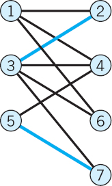
Is the matching M1 in Fig. 506a of maximum cardinality? If not, augment it until maximum cardinality is reached.

Fig. 506. Example 1
Solution. We apply the algorithm.
- 1. Label 1 and 4 with Ø
- 2. Label 7 with 1. Label 5, 6, 8 with 3.
- 3. Label 2 with 6, and 3 with 7.
[All vertices are now labeled as shown in Fig.506a.]
- 4. p1: 1 − 7 − 3 − 5. [By backtracking, P1 is augmenting.]
p2: 1 − 7 − 3 − 8. [p2 is augmenting.]
- 5. Augment M1 by using p1, dropping (3, 7) from M1 and including (1, 7) and (3, 5).Remove all labels. Go to Step 1.
Figure 506b shows the resulting matching M2 = {(1, 7), (2, 6), (3, 5)}.
- 1. Label 4 with Ø
- 2. Label 7 with 2. Label 6 and 8 with 3.
- 3. Label 1 with 7, and 2 with 6, and 3 with 5.
- 4. p3: 5 − 3 − 8. [p3 is alternating but not augmenting.]
- 5. Stop. M2 is of maximum cardinality (namely, 3).
1–7 BIPARTITE OR NOT?
If you answer is yes, find S and T:


- Can you obtain the answer to Prob. 3 from that to Prob. 1?
- Can you obtain a bipartite subgraph in Prob. 4 by omitting two edges? Any two edges? Any two edges without a common vertex?
10–12 MATCHING. AUGMENTING PATHS
Find an augmenting path:
- 10.

- 11.
- 12.

13–15 MAXIMUM CARDINALITY MATCHING
Using augmenting paths, find a maximum cardinality matching:
- 13. In Prob. 11
- 14. In Prob. 10
- 15. In Prob. 12
- 16. Complete bipartite graphs. A bipartite graph G = (S, T; E) is called complete if every vertex in S is joined to every vertex in T by an edge, and is denoted by Kn1,n2, where n1 and n2 are the numbers of vertices in S and T, respectively. How many edges does this graph have?
- 17. Planar graph. A planar graph is a graph that can be drawn on a sheet of paper so that no two edges cross. Show that the complete graph K4 with four vertices is planar. The complete graph K5 with five vertices is not planar. Make this plausible by attempting to draw K5 so that no edges cross. Interpret the result in terms of a net of roads between five cities.
- 18. Bipartite graph K3,3 not planar. Three factories 1, 2, 3 are each supplied underground by water, gas, and electricity, from points A, B, C, respectively. Show that this can be represented by K3,3 (the complete bipartite graph G = (S, T; E) with S and T consisting of three vertices each) and that eight of the nine supply lines (edges) can be laid out without crossing. Make it plausible that K3,3 is not planar by attempting to draw the ninth line without crossing the others.
19–25 VERTEX COLORING
- 19. Vertex coloring and exam scheduling. What is the smallest number of exam periods for six subjects a, b, c, d, e, f if some of the students simultaneously take a, b, f, some c, d, e, some a, c, e, and some c, e? Solve this as follows. Sketch a graph with six vertices a, …, f and join vertices if they represent subjects simultaneously taken by some students. Color the vertices so that adjacent vertices receive different colors. (Use numbers 1, 2, … instead of actual colors if you want.) What is the minimum number of colors you need? For any graph G, this minimum number is called the (vertex) chromatic number Xν(G). Why is this the answer to the problem? Write down a possible schedule.
- 20. Scheduling and matching. Three teachers x1, x2, x3 teach four classes y1, y2, y3, y4 for these numbers of periods:
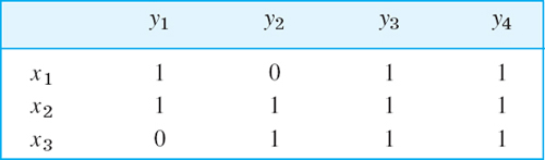
Show that this arrangement can be represented by a bipartite graph G and that a teaching schedule for one period corresponds to a matching in G. Set up a teaching schedule with the smallest possible number of periods.
- 21. How many colors do you need for vertex coloring any tree?
- 22. Harbor management. How many piers does a harbor master need for accommodating six cruise ships S1, …, S6 with expected dates of arrival A and departure D in July, (A, D) = (10, 13), (13, 15), (14, 17), (12, 15), (16, 18), (14, 17), respectively, if each pier can accommodate only one ship, arrival being at 6 am and departures at 11 pm? Hint. Join Si and Sj by an edge if their intervals overlap. Then color vertices.
- 23. What would be the answer to Prob. 22 if only the five ships S1, …, S5 had to be accommodated?
- 24. Four- (vertex) color theorem. The famous four-color theorem states that one can color the vertices of any planar graph (so that adjacent vertices get different colors) with at most four colors. It had been conjectured for a long time and was eventually proved in 1976 by Appel and Haken [Illinois J. Math 21 (1977), 429–567]. Can you color the complete graph K5 with four colors? Does the result contradict the four-color theorem? (For more details, see Ref. [F1] in App. 1.)
- 25. Find a graph, as simple as possible, that cannot be vertex colored with three colors. Why is this of interest in connection with Prob. 24?
- 26. Edge coloring. The edge chromatic number Xe(G) of a graph G is the minimum number of colors needed for coloring the edges of G so that incident edges get different colors. Clearly, Xe(G)
 max d(u), where d(u) is the degree of vertex u. If G = (S, T, E) is bipartite, the equality sign holds. Prove this for Kn,n the complete (cf. Sec. 23.1) bipartite graph G = (S, T, E) with S and T consisting of n vertices each.
CHAPTER 23 REVIEW QUESTIONS AND PROBLEMS
- What is a graph, a digraph, a cycle, a tree?
- State some typical problems that can be modeled and solved by graphs or digraphs.
- State from memory how graphs can be handled on computers.
- What is a shortest path problem? Give applications.
- What situations can be handled in terms of the traveling salesman problem?
- Give typical applications involving spanning trees.
- What are the basic ideas and concepts in handling flows?
- What is combinatorial optimization? Which sections of this chapter involved it? Explain details.
- Define bipartite graphs and describe some typical applications of them.
- What is BFS? DFS? In what connection did these concepts occur?
11–16 MATRICES FOR GRAPHS AND DIGRAPHS
Find the adjacency matrix of:
- 11.

- 12.

- 13.

14–16 Sketch the graph whose adjacency matrix is:
- 14.

- 15.

- 16.

- 17. Vertex incidence list. Make it for the graph in Prob. 15.
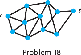
- 18. Find a shortest path and its length by Moore's BFS algorithm, assuming that all the edges have length 1.
- 19. Find shortest paths by Dijkstra's algorithm.

- 20. Find a shortest spanning tree.

- 21. Company A has offices in Chicago, Los Angeles, and New York; Company B in Boston and New York; Company C in Chicago, Dallas, and Los Angeles. Represent this by a bipartite graph.
- 22. Find flow augmenting paths and the maximum flow.

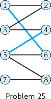
- 23. Using augmenting paths, find a maximum cardinality matching.
- 24. Find an augmenting path,

SUMMARY OF CHAPTER 23
Graphs. Combinatorial Optimization
Combinatorial optimization concerns optimization problems of a discrete or combinatorial structure. It uses graphs and digraphs (Sec. 23.1) as basic tools.
A graph G = (V, E) consists of a set V of vertices ν1, ν2, …, νn (often simply denoted by 1, 2, …, n) and a set E of edges e1, e2, …, em, each of which connects two vertices. We also write (i, j) for an edge with vertices i and j as endpoints. A digraph (= directed graph) is a graph in which each edge has a direction (indicated by an arrow). For handling graphs and digraphs in computers, one can use matrices or lists (Sec. 23.1).
This chapter is devoted to important classes of optimization problems for graphs and digraphs that all arise from practical applications, and corresponding algorithms, as follows.
In a shortest path problem (Sec. 23.2) we determine a path of minimum length (consisting of edges) from a vertex s to a vertex t in a graph whose edges (i, j) have a “length” lij > 0, which may be an actual length or a travel time or cost or an electrical resistance [if (i, j) is a wire in a net], and so on. Dijkstra's algorithm (Sec. 23.3) or, when all lij = 1, Moore's algorithm (Sec. 23.2) are suitable for these problems.
A tree is a graph that is connected and has no cycles (no closed paths). Trees are very important in practice. A spanning tree in a graph G is a tree containing all the vertices of G. If the edges of G have lengths, we can determine a shortest spanning tree, for which the sum of the lengths of all its edges is minimum, by Kruskal's algorithm or Prim's algorithm (Secs. 23.4, 23.5).
A network (Sec. 23.6) is a digraph in which each edge (i, j) has a capacity cij > 0 [= maximum possible flow along (i, j)] and at one vertex, the source s, a flow is produced that flows along the edges to a vertex t, the sink or target, where the flow disappears. The problem is to maximize the flow, for instance, by applying the Ford–Fulkerson algorithm (Sec. 23.7), which uses flow augmenting paths (Sec. 23.6). Another related concept is that of a cut set, as defined in Sec. 23.6.
A bipartite graph G = (V, E) (Sec. 23.8) is a graph whose vertex set V consists of two parts S and T such that every edge of G has one end in S and the other in T, so that there are no edges connecting vertices in S or vertices in T. A matching in G is a set of edges, no two of which have an endpoint in common. The problem then is to find a maximum cardinality matching in G, that is, a matching M that has a maximum number of edges. For an algorithm, see Sec. 23.8.
1WILLIAM ROWAN HAMILTON (1805–1865), Irish mathematician, known for his work in dynamics.
2EDWARD FORREST MOORE (1925–2003), American mathematician and computer scientist, who did pioneering work in theoretical computer science (automata theory, Turing machines).
3RICHARD BELLMAN (1920–1984), American mathematician, known for his work in dynamic programming.
4EDSGER WYBE DIJKSTRA (1930–2002), Dutch computer scientist, 1972 recipient of the ACM Turing Award. His algorithm appeared in Numerische Mathematik1 (1959), 269–271.
5JOSEPH BERNARD KRUSKAL (1928–), American mathematician who worked at Bell Laboratories. He is known for his contributions to graph theory and statistics.
6ROBERT CLAY PRIM (1921–), American computer scientist at General Electric, Bell Laboratories, and Sandia National Laboratories.
7LESTER RANDOLPH FORD Jr. (1927–) and DELBERT RAY FULKERSON (1924–1976), American mathematicians known for their pioneering work on flow algorithms.