
CHAPTER 22
Unconstrained Optimization.
Linear Programming
Optimization is a general term used to describe types of problems and solution techniques that are concerned with the best (“optimal”) allocation of limited resources in projects. The problems are called optimization problems and the methods optimization methods. Typical problems are concerned with planning and making decisions, such as selecting an optimal production plan. A company has to decide how many units of each product from a choice of (distinct) products it should make. The objective of the company may be to maximize overall profit when the different products have different individual profits. In addition, the company faces certain limitations (constraints). It may have a certain number of machines, it takes a certain amount of time and usage of these machines to make a product, it requires a certain number of workers to handle the machines, and other possible criteria. To solve such a problem, you assign the first variable to number of units to be produced of the first product, the second variable to the second product, up to the number of different (distinct) products the company makes. When you multiply these, for example, by the price, you obtain a linear function called the objective function. You also express the constraints in terms of these variables, thereby obtaining several inequalities, called the constraints. Because the variables in the objective function also occur in the constraints, the objective function and the constraints are tied mathematically to each other and you have set up a linear optimization problem, also called a linear programming problem.
The main focus of this chapter is to set up (Sec. 22.2) and solve (Secs. 22.3, 22.4) such linear programming problems. A famous and versatile method for doing so is the simplex method. In the simplex method, the objective function and the constraints are set up in the form of an augmented matrix as in Sec. 7.3, however, the method of solving such linear constrained optimization problems is a new approach.
The beauty of the simplex method is that it allows us to scale problems up to thousands or more constraints, thereby modeling real-world situations. We can start with a small model and gradually add more and more constraints. The most difficult part is modeling the problem correctly. The actual task of solving large optimization problems is done by software implementations for the simplex method or perhaps by other optimization methods.
Besides optimal production plans, problems in optimal shipping, optimal location of warehouses and stores, easing traffic congestion, efficiency in running power plants are all examples of applications of optimization. More recent applications are in minimizing environmental damages due to pollutants, carbon dioxide emissions, and other factors. Indeed, new fields of green logistics and green manufacturing are evolving and naturally make use of optimization methods.
Prerequisite: a modest working knowledge of linear systems of equations.
References and Answers to Problems: App. 1 Part F, App. 2.
22.1 Basic Concepts.
Unconstrained Optimization:
Method of Steepest Descent
In an optimization problem the objective is to optimize (maximize or minimize) some function f. This function f is called the objective function. It is the focal point or goal of our optimization problem.
For example, an objective function f to be maximized may be the revenue in a production of TV sets, the rate of return of a financial portfolio, the yield per minute in a chemical process, the mileage per gallon of a certain type of car, the hourly number of customers served in a bank, the hardness of steel, or the tensile strength of a rope.
Similarly, we may want to minimize f if f is the cost per unit of producing certain cameras, the operating cost of some power plant, the daily loss of heat in a heating system, CO2 emissions from a fleet of trucks for freight transport, the idling time of some lathe, or the time needed to produce a fender.
In most optimization problems the objective function f depends on several variables
![]()
These are called control variables because we can “control” them, that is, choose their values.
For example, the yield of a chemical process may depend on pressure x1 and temperature x2. The efficiency of a certain air-conditioning system may depend on temperature x1, air pressure x2, moisture content x3, cross-sectional area of outlet x4, and so on.
Optimization theory develops methods for optimal choices of x1, …, xn, which maximize (or minimize) the objective function f, that is, methods for finding optimal values of x1, …, xn.
In many problems the choice of values of x1, …, xn is not entirely free but is subject to some constraints, that is, additional restrictions arising from the nature of the problem and the variables.
For example, if x1 is production cost, then ![]() , and there are many other variables (time, weight, distance traveled by a salesman, etc.) that can take nonnegative values only. Constraints can also have the form of equations (instead of inequalities).
, and there are many other variables (time, weight, distance traveled by a salesman, etc.) that can take nonnegative values only. Constraints can also have the form of equations (instead of inequalities).
We first consider unconstrained optimization in the case of a function f(x1, …, xn). We also write X = (x1, …, xn) and f(x), for convenience.
By definition, f has a minimum at a point x = X0 in a region R (where f is defined) if
![]()
for all x in R. Similarly, f has a maximum at X0 in R if
![]()
for all x in R. Minima and maxima together are called extrema.
Furthermore, f is said to have a local minimum at X0 if
![]()
for all x in a neighborhood of X0, say, for all x satisfying
![]()
where X0 = (X1, …, Xn) and r > 0 is sufficiently small.
Similarly, f has a local maximum at X0 if ![]() for all x satisfying |x − X0| < r.
for all x satisfying |x − X0| < r.
If f is differentiable and has an extremum at a point X0 in the interior of a region R (that is, not on the boundary), then the partial derivatives ∂f/∂x1, …, ∂f/∂xn must be zero at X0. These are the components of a vector that is called the gradient of f and denoted by grad f or ∇f. (For n = 3 this agrees with Sec. 9.7.) Thus

A point X0 at which (1) holds is called a stationary point of f.
Condition (1) is necessary for an extremum of f at X0 in the interior of R, but is not sufficient. Indeed, if, n = 1, then for y = f(x), condition (1) is y′ = f′(X0) = 0; and, for instance, y = x3 satisfies y′ = 3x2 = 0 at x = X0 = 0 where f has no extremum but a point of inflection. Similarly, for f(x) = x1x2 we have δf(0) = 0, and f does not have an extremum but has a saddle point at 0. Hence, after solving (1), one must still find out whether one has obtained an extremum. In the case n = 1 the conditions y′(X0) = 0, y″(X0) > 0 guarantee a local minimum at X0 and the conditions y′(X0) = 0, y″(X0) < 0 a local maximum, as is known from calculus. For n > 1 there exist similar criteria. However, in practice, even solving (1) will often be difficult. For this reason, one generally prefers solution by iteration, that is, by a search process that starts at some point and moves stepwise to points at which f is smaller (if a minimum of f is wanted) or larger (in the case of a maximum).
The method of steepest descent or gradient method is of this type. We present it here in its standard form. (For refinements see Ref. [E25] listed in App. 1.)
The idea of this method is to find a minimum of f(x) by repeatedly computing minima of a function g(t) of a single variable t, as follows. Suppose that f has a minimum at X0 and we start at a point x. Then we look for a minimum of f closest to x along the straight line in the direction of ![]() , which is the direction of steepest descent (= direction of maximum decrease) of f at x. That is, we determine the value of t and the corresponding point
, which is the direction of steepest descent (= direction of maximum decrease) of f at x. That is, we determine the value of t and the corresponding point
![]()
at which the function
![]()
has a minimum. We take this z(t)as our next approximation to X0.
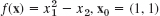
EXAMPLE 1 Method of Steepest Descent
Determine a minimum of
![]()
starting from x0 = (6, 3) = 6i + 3j and applying the method of steepest descent.
Solution. Clearly, inspection shows that f(x) has a minimum at 0. Knowing the solution gives us a better feel of how the method works. We obtain ![]() and from this
and from this

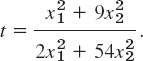
We now calculate the derivative
![]()
set g′(t) = 0, and solve for t, finding
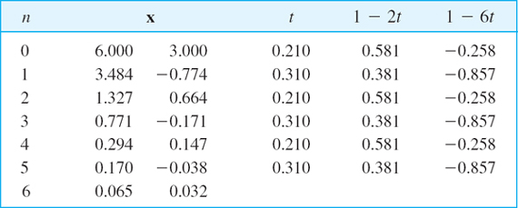
Starting from x0 = 6i + 3j, we compute the values in Table 22.1, which are shown in Fig. 473.
Figure 473 suggests that in the case of slimmer ellipses (“a long narrow valley”), convergence would be poor. You may confirm this by replacing the coefficient 3 in (4) with a large coefficient. For more sophisticated descent and other methods, some of them also applicable to vector functions of vector variables, we refer to the references listed in Part F of App. 1; see also [E25].

Fig. 473. Method of steepest descent in Example 1
Table 22.1 Method of Steepest Descent, Computations in Example 1
- Orthogonality. Show that in Example 1, successive gradients are orthogonal (perpendicular). Why?
- What happens if you apply the method of steepest descent to
 ? First guess, then calculate.
3–9 STEEPEST DESCENT
Do steepest descent steps when:
- 3.
 , x0 = 0, 3 steps
 - 4.
 , x0 = (3, 4), 5 steps
 - 5. f(x) = zx1 + bx2, a ≠ 0, b ≠ 0. First guess, then compute.
- 6.
 , 5 steps. First guess, then compute. Sketch the path. What if x0 = (2, 1)?
 - 7.
 . Show that 2 steps give (c, 1) times a factor, −4c2/(c2 − 1)2. What can you conclude from this about the speed of convergence?
 - 8.
 ; 3 steps. Sketch your path. Predict the outcome of further steps.
 - 9.
 x0 = (3, 3), 5 steps
 - 10. CAS EXPERIMENT. Steepest Descent.
- Write a program for the method.
- Apply your program to
 experimenting with respect to speed of convergence depending on the choice of x0.
 - Apply your program to
 and to
 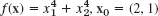 . Graph level curves and your path of descent. (Try to include graphing directly in your program.)
22.2 Linear Programming
Linear programming or linear optimization consists of methods for solving optimization problems with constraints, that is, methods for finding a maximum (or a minimum) x = (x1, …, xn) of a linear objective function
![]()
satisfying the constraints. The latter are linear inequalities, such as 3x1 + 4x2 ![]() 36, or x1
36, or x1 ![]() 0, etc. (examples below). Problems of this kind arise frequently, almost daily, for instance, in production, inventory management, bond trading, operation of power plants, routing delivery vehicles, airplane scheduling, and so on. Progress in computer technology has made it possible to solve programming problems involving hundreds or thousands or more variables. Let us explain the setting of a linear programming problem and the idea of a “geometric” solution, so that we shall see what is going on.
0, etc. (examples below). Problems of this kind arise frequently, almost daily, for instance, in production, inventory management, bond trading, operation of power plants, routing delivery vehicles, airplane scheduling, and so on. Progress in computer technology has made it possible to solve programming problems involving hundreds or thousands or more variables. Let us explain the setting of a linear programming problem and the idea of a “geometric” solution, so that we shall see what is going on.
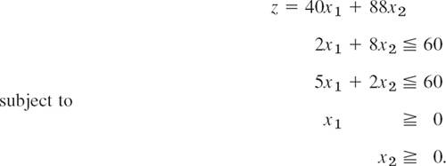
Energy Savers, Inc., produces heaters of types S and L. The wholesale price is $40 per heater for S and $88 for L. Two time constraints result from the use of two machines M1 and M2. On M1 one needs 2 min for an S heater and 8 min for an L heater. On M2 one needs 5 min for an S heater and 2 min for an L heater. Determine production figures x1 and x2 for S and L, respectively (number of heaters produced per hour), so that the hourly revenue
![]()
is maximum.
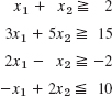
Solution. Production figures x1 and x2 must be nonnegative. Hence the objective function (to be maximized) and the four constraints are
![]()
![]()
![]()
![]()
![]()
Figure 474 shows (0)–(4) as follows. Constancy lines
![]()
are marked (0). These are lines of constant revenue. Their slope is −40/88 = −5/11. To increase z we must move the line upward (parallel to itself), as the arrow shows. Equation (1) with the equality sign is marked (1). It intersects the coordinate axes at x1 = 60/2 = 30 (set x2 = 0) and x2 = 60/8 = 7.5 (set x1 = 0). The arrow marks the side on which the points (x1, x2) lie that satisfy the inequality in (1). Similarly for Eqs. (2)–(4). The blue quadrangle thus obtained is called the feasibility region. It is the set of all feasible solutions, meaning solutions that satisfy all four constraints. The figure also lists the revenue at O, A, B, C. The optimal solution is obtained by moving the line of constant revenue up as much as possible without leaving the feasibility region completely. Obviously, this optimum is reached when that line passes through B, the intersection (10, 5) of (1) and (2). We see that the optimal revenue
![]()
is obtained by producing twice as many S heaters as L heaters.

Fig. 474. Linear programming in Example 1
Note well that the problem in Example 1 or similar optimization problems cannot be solved by setting certain partial derivatives equal to zero, because crucial to such problems is the region in which the control variables are allowed to vary.
Furthermore, our “geometric” or graphic method illustrated in Example 1 is confined to two variables x1, x2. However, most practical problems involve much more than two variables, so that we need other methods of solution.
Normal Form of a Linear Programming Problem
To prepare for general solution methods, we show that constraints can be written more uniformly. Let us explain the idea in terms of (1),
![]()
This inequality implies 60 − 2x1 − 8x2 ![]() 0 (and conversely), that is, the quantity
0 (and conversely), that is, the quantity
![]()
is nonnegative. Hence, our original inequality can now be written as an equation
![]()
where
![]()
x3 is a nonnegative auxiliary variable introduced for converting inequalities to equations. Such a variable is called a slack variable, because it “takes up the slack” or difference between the two sides of the inequality.
EXAMPLE 2 Conversion of Inequalities by the Use of Slack Variables
With the help of two slack variables x3, x4 we can write the linear programming problem in Example 1 in the following form. Maximize
![]()
subject to the constraints
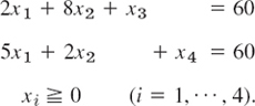
We now have n = 4 variables and m = 2 (linearly independent) equations, so that two of the four variables, for example, x1, x2, determine the others. Also note that each of the four sides of the quadrangle in Fig. 474 now has an equation of the form xi = 0;
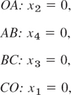
A vertex of the quadrangle is the intersection of two sides. Hence at a vertex, n − m = 4 − 2 = 2 of the variables are zero and the others are nonnegative. Thus at A we have x2 = 0, x4 = 0, and so on.
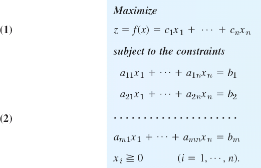
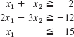
Our example suggests that a general linear optimization problem can be brought to the following normal form. Maximize

subject to the constraints

with all bj nonnegative. (If a bj < 0, multiply the equation by −1.) Here x1, …, xn include the slack variables (for which the cj’s in f are zero). We assume that the equations in (6) are linearly independent. Then, if we choose values for n − m of the variables, the system uniquely determines the others. Of course, since we must have
![]()
this choice is not entirely free.
Our problem also includes the minimization of an objective function f since this corresponds to maximizing −f and thus needs no separate consideration.
An n-tuple (x1, …, xn) that satisfies all the constraints in (6) is called a feasible point or feasible solution. A feasible solution is called an optimal solution if, for it, the objective function f becomes maximum, compared with the values of f at all feasible solutions.
Finally, by a basic feasible solution we mean a feasible solution for which at least n − m of the variables x1, …, xn are zero. For instance, in Example 2 we have n = 4, m = 2, and the basic feasible solutions are the four vertices O, A, B, C in Fig. 474. Here B is an optimal solution (the only one in this example).
The following theorem is fundamental.
Some optimal solution of a linear programming problem (5), (6) is also a basic feasible solution of (5), (6).
For a proof, see Ref. [F5], Chap. 3 (listed in App. 1). A problem can have many optimal solutions and not all of them may be basic feasible solutions; but the theorem guarantees that we can find an optimal solution by searching through the basic feasible solutions only. This is a great simplification; but since there are ![]() different ways of equating n − m of the n variables to zero, considering all these possibilities, dropping those which are not feasible and then searching through the rest would still involve very much work, even when n and m are relatively small. Hence a systematic search is needed. We shall explain an important method of this type in the next section.
different ways of equating n − m of the n variables to zero, considering all these possibilities, dropping those which are not feasible and then searching through the rest would still involve very much work, even when n and m are relatively small. Hence a systematic search is needed. We shall explain an important method of this type in the next section.
1–6 REGIONS, CONSTRAINTS
Describe and graph the regions in the first quadrant of the x1x2-plane determined by the given inequalities.


- Location of maximum. Could we find a profit f(x1, x2) = a1x1 + a2x2 whose maximum is at an interior point of the quadrangle in Fig. 474? Give reason for your answer.
- Slack variables. Why are slack variables always nonnegative? How many of them do we need?
- What is the meaning of the slack variables x3, x4 in Example 2 in terms of the problem in Example 1?
- Uniqueness. Can we always expect a unique solution (as in Example 1)?
11–16 MAXIMIZATION, MINIMIZATION
Maximize or minimize the given objective function f subject to the given constraints.
- 11. Maximize f = 30x1 + 10x2 in the region in Prob. 5.
- 12. Minimize f = 45.0x1 + 22.5x2 in the region in Prob. 4.
- 13. Maximize f = 5x1 + 25x2 in the region in Prob. 5.
- 14. Minimize f = 5x1 + 25x2 in the region in Prob. 3.
- 15. Maximize f = 20x1 + 30x2 subject to 4x1 + 3x2
 12, x1 − x2 −3, x2
  6, 2x1 − 3x2 0.
 - 16. Maximize f = − 10x1 + 2x2 subject to x1 0, x2 0, −x1 + x2 −1, x1 + x2 6, x2 5.
- 17. Maximum profit. United Metal, Inc., produces alloys B1 (special brass) and B2 (yellow tombac). B1 contains 50% copper and 50% zinc. (Ordinary brass contains about 65% copper and 35% zinc.) B2 contains 75% copper and 25% zinc. Net profits are $120 per ton of B1 and $100 per ton of B2. The daily copper supply is 45 tons. The daily zinc supply is 30 tons. Maximize the net profit of the daily production.
- 18. Maximum profit. The DC Drug Company produces two types of liquid pain killer, N (normal) and S (Super). Each bottle of N requires 2 units of drug A, 1 unit of drug B, and 1 unit of drug C. Each bottle of S requires 1 unit of A, 1 unit of B, and 3 units of C. The company is able to produce, each week, only 1400 units of A, 800 units of B, and 1800 units of C. The profit per bottle of N and S is $11 and $15, respectively. Maximize the total profit.
- 19. Maximum output. Giant Ladders, Inc., wants to maximize its daily total output of large step ladders by producing x1 of them by a process p1 and x2 by a process p2, where p1 requires 2 hours of labor and 4 machine hours per ladder, and p2 requires 3 hours of labor and 2 machine hours. For this kind of work, 1200 hours of labor and 1600 hours on the machines are, at most, available per day. Find the optimal x1 and x2.
- 20. Minimum cost. Hardbrick, Inc., has two kilns. Kiln I can produce 3000 gray bricks, 2000 red bricks, and 300 glazed bricks daily. For Kiln II the corresponding figures are 2000, 5000, and 1500. Daily operating costs of Kilns I and II are $400 and $600, respectively. Find the number of days of operation of each kiln so that the operation cost in filling an order of 18,000 gray, 34,000 red, and 9000 glazed bricks is minimized.
- 21. Maximum profit. Universal Electric, Inc., manufactures and sells two models of lamps, L1 and L2, the profit being %150 and $100, respectively. The process involves two workers W1 and W2 who are available for this kind of work 100 and 80 hours per month, respectively. W1 assembles L1 in 20 min and L2 in 30 min. W2 paints L1 in 20 min and L2 in 10 min. Assuming that all lamps made can be sold without difficulty, determine production figures that maximize the profit.
- 22. Nutrition. Foods A and B have 600 and 500 calories, contain 15 g and 30 g of protein, and cost $1.80 and $2.10 per unit, respectively. Find the minimum cost diet of at least 3900 calories containing at least 150 g of protein.
22.3 Simplex Method
From the last section we recall the following. A linear optimization problem (linear programming problem) can be written in normal form; that is:
For finding an optimal solution of this problem, we need to consider only the basic feasible solutions (defined in Sec. 22.2), but there are still so many that we have to follow a systematic search procedure. In 1948 G. B. Dantzig1 published an iterative method, called the simplex method, for that purpose. In this method, one proceeds stepwise from one basic feasible solution to another in such a way that the objective function f always increases its value. Let us explain this method in terms of the example in the last section.
In its original form the problem concerned the maximization of the objective function
Converting the first two inequalities to equations by introducing two slack variables x3, x4, we obtained the normal form of the problem in Example 2. Together with the objective function (written as an equation z − 40x1 − 88x2 = 0) this normal form is

where x1 ![]() 0, …, x4
0, …, x4 ![]() 0. This is a linear system of equations. To find an optimal solution of it, we may consider its augmented matrix (see Sec. 7.3)
0. This is a linear system of equations. To find an optimal solution of it, we may consider its augmented matrix (see Sec. 7.3)
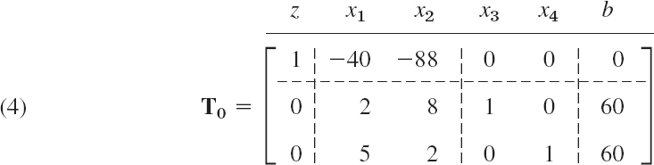
This matrix is called a simplex tableau or simplex table (the initial simplex table). These are standard names. The dashed lines and the letters
![]()
are for ease in further manipulation.
Every simplex table contains two kinds of variables xj. By basic variables we mean those whose columns have only one nonzero entry. Thus x3, x4 in (4) are basic variables and x1, x2 are nonbasic variables.
Every simplex table gives a basic feasible solution. It is obtained by setting the nonbasic variables to zero. Thus (4) gives the basic feasible solution
![]()
with x3 obtained from the second row and x4 from the third.
The optimal solution (its location and value) is now obtained stepwise by pivoting, designed to take us to basic feasible solutions with higher and higher values of z until the maximum of z is reached. Here, the choice of the pivot equation and pivot are quite different from that in the Gauss elimination. The reason is that x1, x2, x3, x4 are restricted to nonnegative values.
Step 1. Operation O1: Selection of the Column of the Pivot
Select as the column of the pivot the first column with a negative entry in Row 1. In (4) this is Column 2 (because of the −40).
Operation O2: Selection of the Row of the Pivot. Divide the right sides [60 and 60 in (4)] by the corresponding entries of the column just selected (60/2 = 30, 60/5 = 12). Take as the pivot equation the equation that gives the smallest quotient. Thus the pivot is 5 because 60/5 is smallest.
Operation O3: Elimination by Row Operations. This gives zeros above and below the pivot (as in Gauss–Jordan, Sec. 7.8).
With the notation for row operations as introduced in Sec. 7.3, the calculations in Step 1 give from the simplex table T0 in (4) the following simplex table (augmented matrix), with the blue letters referring to the previous table.

We see that basic variables are now x1, x3 and nonbasic variables are x2, x4. Setting the latter to zero, we obtain the basic feasible solution given by T1,
![]()
This is A in Fig. 474 (Sec. 22.2). We thus have moved from o: (0, 0) with z = 0 to A: (12, 0) with the greater z = 480. The reason for this increase is our elimination of a term (−40x1) with a negative coefficient. Hence elimination is applied only to negative entries in Row 1 but to no others. This motivates the selection of the column of the pivot.
We now motivate the selection of the row of the pivot. Had we taken the second row of T0 instead (thus 2 as the pivot), we would have obtained z = 1200 (verify!), but this line of constant revenue z = 1200 lies entirely outside the feasibility region in Fig. 474. This motivates our cautious choice of the entry 5 as our pivot because it gave the smallest quotient (60/5 = 12).
Step 2. The basic feasible solution given by (5) is not yet optimal because of the negative entry −72 in Row 1. Accordingly, we perform the operations O1 to O3 again, choosing a pivot in the column of −72.
Operation O1. Select Column 3 of T1 in (5) as the column of the pivot (because −72 < 0).
Operation O2. We have 36/7.2 = 5 and 60/2 = 30. Select 7.2 as the pivot (because 5 < 30).
Operation O3. Elimination by row operations gives
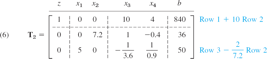
We see that now x1, x2 are basic and x3, x4 nonbasic. Setting the latter to zero, we obtain from T2 the basic feasible solution
![]()
This is B in Fig. 474 (Sec. 22.2). In this step, z has increased from 480 to 840, due to the elimination of −72 in T1. Since T2 contains no more negative entries in Row 1, we conclude that z = f(10, 5) = 40 · 10 + 88 · 5 = 840 is the maximum possible revenue. It is obtained if we produce twice as many S heaters as L heaters. This is the solution of our problem by the simplex method of linear programming.
Minimization. If we want to minimize z = f(x) (instead of maximize), we take as the columns of the pivots those whose entry in Row 1 is positive (instead of negative). In such a Column k we consider only positive entries tjk and take as pivot a tjk for which bj/tjk is smallest (as before). For examples, see the problem set.
- Verify the calculations in Example 1 of the text.
2–14 SIMPLEX METHOD
Write in normal form and solve by the simplex method, assuming all xj to be nonnegative.
- 2. The problem in the example in the text with the constraints interchanged.
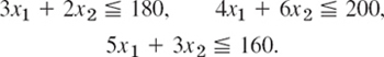
- 3. Maximize f = 3x1 + 2x2 subject to 3x1 + 4x2 60, 4x1 + 3x2 60, 10x1 + 2x2 120.
- 4. Maximize the daily output in producing x1 chairs by Process p1 and x2 chairs by Process p2 subject to 3x1 + 4x2 550 (machine hours), 5x1 + 4x2 650 (labor).
- 5. Minimize f = 5x1 − 20x2 subject to −2x1 + 10x2 5, 2x1 + 5x2 10.
- 6. Prob. 19 in Sec. 22.2.
- 7. Suppose we produce x1 AA batteries by process P1 and x2 by Process P2, furthermore x3 A batteries by Process P3 and x4 by Process P4. Let the profit for 100 batteries be $10 for AA and $20 for A. Maximize the total profit subject to the constraints

- 8. Maximize the daily profit in producing x1 metal frames F1 (profit $90 per frame) and x2 frames F2 (profit $50 per frame) subject to x1 + 3x2 18 (material), x1 + x2 10 (machine hours), 3x1 + x2 24 (labor).
- 9. Maximize f = 2x1 + x2 + 3x3 subject to 4x1 + 3x2 + 6x3 = 12.
- 10. Minimize f = 4x1 − 10x2 − 20x3 subject to 3x1 + 4x2 + 5x3 60, 2x1 + x2 20, 2x1 + 3x3 30.
- 11. Prob. 22 in Problem Set 22.2.
- 12. Maximize f = 2x1 + 3x2 + x3 subject to x1 + x2 + x3 4.8, 10x1 + x3 9.9, x2 − x3 0.2.
- 13. Maximize f = 34x1 + 29x2 + 32x3 subject to 8x1 + 2x2 + x3 54, 3x1 + 8x2 + 2x3 59, x1 + x2 + 5x3 39.
- 14 Maximize f = 2x1 + 3x2 subject to 5x1 + 3x2 105, 3x1 + 6x2 126.
- 15. CAS PROJECT. Simple Method. (a) Write a program for graphing a region R in the first quadrant of the x1x2-plane determined by linear constraints.
(b) Write a program for maximizing z = a1x1 + a2x2 in R.
(c) Write a program for maximizing z = a1x1 + … + anxn subject to linear constraints.
(d) Apply your programs to problems in this problem set and the previous one.
22.4 Simplex Method: Difficulties
In solving a linear optimization problem by the simplex method, we proceed stepwise from one basic feasible solution to another. By so doing, we increase the value of the objective function f. We continue this stepwise procedure, until we reach an optimal solution. This was all explained in Sec. 22.3. However, the method does not always proceed so smoothly. Occasionally, but rather infrequently in practice, we encounter two kinds of difficulties. The first one is the degeneracy and the second one concerns difficulties in starting.
Degeneracy
A degenerate feasible solution is a feasible solution at which more than the usual number n − m of variables are zero. Here n is the number of variables (slack and others) and m the number of constraints (not counting the xj ![]() 0 conditions). In the last section, n = 4 and m = 2, and the occurring basic feasible solutions were nondegenerate; n − m = 2 variables were zero in each such solution.
0 conditions). In the last section, n = 4 and m = 2, and the occurring basic feasible solutions were nondegenerate; n − m = 2 variables were zero in each such solution.
In the case of a degenerate feasible solution we do an extra elimination step in which a basic variable that is zero for that solution becomes nonbasic (and a nonbasic variable becomes basic instead). We explain this in a typical case. For more complicated cases and techniques (rarely needed in practice) see Ref. [F5] in App. 1.
EXAMPLE 1 Simplex Method, Degenerate Feasible Solution
AB Steel, Inc., produces two kinds of iron I1, I2 by using three kinds of raw material R1, R2, R3 (scrap iron and two kinds of ore) as shown. Maximize the daily profit.

Solution. Let x1 and x2 denote the amount (in tons) of iron I1 and I2, respectively, produced per day. Then our problem is as follows. Maximize
![]()
subject to the constraints x1 ![]() 0, x2
0, x2 ![]() 0 and
0 and
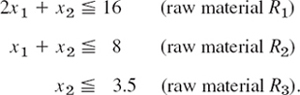
By introducing slack variables x3, x4, x5 we obtain the normal form of the constraints

As in the last section we obtain from (1) and (2) the initial simplex table

We see that x1, x2 are nonbasic variables and x3, x4, x5 are basic. With x1 = x2 = 0 we have from (3) the basic feasible solution
![]()
This is in Fig. 475. We have n = 5 variables xj, m = 3 constraints, and n − m = 2 variables equal to zero in our solution, which thus is nondegenerate.
Step 1 of Pivoting
Operation O1: Column Selection of Pivot. Column 2 (since − 150 < 0).
Operation O2: Row Selection of Pivot. 16/2 = 8, 8/1 = 8; 3.5/0 is not possible. Hence we could choose Row 2 or Row 3. We choose Row 2. The pivot is 2.
Operation O3: Elimination by Row Operations. This gives the simplex table

We see that the basic variables are x1, x4, x5 and the nonbasic are x2, x3 Setting the nonbasic variables to zero, we obtain from T1 the basic feasible solution

Fig. 475. Example 1, where A is degenerate
![]()
This is A: (8, 0) in Fig. 475. This solution in degenerate because x4 = 0 (in addition to x2 = 0, x3 = 0); geometrically: the straight line x4 = 0 also passes through A. This requires the next step, in which x4 will become nonbasic.
Step 2 of Pivoting
Operation O1: Column Selection of Pivot. Column 3 (since − 225 < 0).
Operation O2: Row Selection of Pivot. ![]() . Hence
. Hence ![]() must serve as the pivot.
must serve as the pivot.
Operation O3: Elimination by Row Operations. This gives the following simplex table.
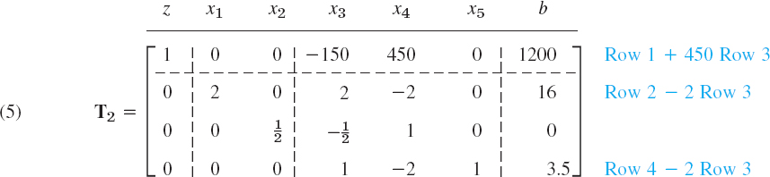
We see that the basic variables are x1, x2, x5 and the nonbasic are x3, x4. Hence x4 has become nonbasic, as intended. By equating the nonbasic variables to zero we obtain from T2 the basic feasible solution
![]()
This is still A: (8, 0) in Fig. 475 and z has not increased. But this opens the way to the maximum, which we reach in the next step.
Operation O1: Column Selection of Pivot. Column 4 (since − 150 < 0).
Operation O2: Row Selection of Pivot. ![]() . We can take 1 as the pivot. (With
. We can take 1 as the pivot. (With ![]() as the pivot we would not leave A. Try it.)
as the pivot we would not leave A. Try it.)
Operation O3: Elimination by Row Operations. This gives the simplex table

We see that basic variables are x1, x2, x3 and nonbasic x4, x5. Equating the latter to zero we obtain from T3 the basic feasible solution
![]()
This is B: (4.5, 3.5) in Fig. 475. Since Row 1 of T3 has no negative entries, we have reached the maximum daily profit zmax = f(4.5, 3.5) = 150 · 4.5 + 300 · 3.5 = $1725. This is obtained by using 4.5 tons of iron I1 and 3.5 tons of iron I2.
Difficulties in Starting
As a second kind of difficulty, it may sometimes be hard to find a basic feasible solution to start from. In such a case the idea of an artificial variable (or several such variables) is helpful. We explain this method in terms of a typical example.
EXAMPLE 2 Simplex Method: Difficult Start, Artificial Variable
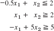
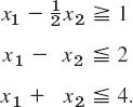
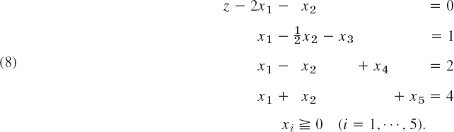
Maximize
![]()
subject to the constraints x1 ![]() 0, x2
0, x2 ![]() 0 and (Fig. 476)
0 and (Fig. 476)
Solution. By means of slack variables we achieve the normal form of the constraints
Note that the first slack variable is negative (or zero), which makes x3 nonnegative within the feasibility region (and negative outside). From (7) and (8) we obtain the simplex table
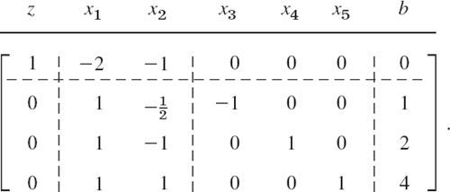
x1, x2 are nonbasic, and we would like to take x3, x4, x5 as basic variables. By our usual process of equating the nonbasic variables to zero we obtain from this table
![]()
x3 < 0 indicates that (0, 0) lies outside the feasibility region. Since x3 < 0, we cannot proceed immediately. Now, instead of searching for other basic variables, we use the following idea. Solving the second equation in (8) for x3, we have
![]()
To this we now add a variable x6 on the right,

Fig. 476. Feasibility region in Example 2
![]()
x6 is called an artificial variable and is subject to the constraint x6 ![]() 0.
0.
We must take care that x6 (which is not part of the given problem!) will disappear eventually. We shall see that we can accomplish this by adding a term −Mx6 with very large M to the objective function. Because of (7) and (9) (solved for x6) this gives the modified objective function for this “extended problem”
![]()
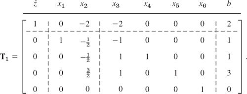
We see that the simplex table corresponding to (10) and (8) is

The last row of this table results from (9) written as ![]() . We see that we can now start, taking x4, x5, x6 as the basic variables and x1, x2, x3 as the nonbasic variables. Column 2 has a negative first entry. We can take the second entry (1 in Row 2) as the pivot. This gives
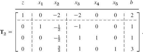
. We see that we can now start, taking x4, x5, x6 as the basic variables and x1, x2, x3 as the nonbasic variables. Column 2 has a negative first entry. We can take the second entry (1 in Row 2) as the pivot. This gives
This corresponds to x1 = 1, x2 = 0 (point A in Fig. 476), x3 = 0, x4 = 1, x5 = 3, x6 = 0. We can now drop Row 5 and Column 7. In this way we get rid of x6, as wanted, and obtain
In Column 3 we choose ![]() as the next pivot. We obtain
as the next pivot. We obtain

This corresponds to x1 = 2, x2 = 2 (this is B in Fig. 476), x3 = 0, x4 = 2, 2, x5 = 0. In Column 4 we choose ![]() as the pivot, by the usual principle. This gives
as the pivot, by the usual principle. This gives

This corresponds to x1 = 3, x2 = 1 (point C in Fig. 476), ![]() . This is the maximum fmax = f(3, 1) = 7.
. This is the maximum fmax = f(3, 1) = 7.
We have reached the end of our discussion on linear programming. We have presented the simplex method in great detail as this method has many beautiful applications and works well on most practical problems. Indeed, problems of optimization appear in civil engineering, chemical engineering, environmental engineering, management science, logistics, strategic planning, operations management, industrial engineering, finance, and other areas. Furthermore, the simplex method allows your problem to be scaled up from a small modeling attempt to a larger modeling attempt, by adding more constraints and variables, thereby making your model more realistic. The area of optimization is an active field of development and research and optimization methods, besides the simplex method, are being explored and experimented with.
- Maximize z = f1(x) = 7x1 + 14x2 subject to 0 x1 6, 0 x2 3, 7x1 + 14x2 84.
- Do Prob. 1 with the last two constraints interchanged.
- Maximize the daily output in producing x1 steel sheets by process pA and x2 steel sheets by process pB subject to the constraints of labor hours, machine hours, and raw material supply:
- Maximize z = 300x1 + 500x2 subject to 2x1 + 8x2 60, 2x1 + x2 30, 4x1 + 4x2 60.
- Do Prob. 4 with the last two constraints interchanged. Comment on the resulting simplification.
- Maximize the total output f = x1 + x2 + x3 (production from three distinct processes) subject to input constraints (limitation of time available for production)

- Maximize f = 5x1 + 8x2 + 4x3 subject to xj 0 (j = 1, …, 5) and x1 + x3 + x5 = 1, x2 + x3 + x4 = 1.
- Using an artificial variable, minimize f = 4x1 − x2 subject to x1 + x2 2, −2x1 + 3x2 1, 5x1 + 4x2 50.
- Maximize f = 2x1 + 3x2 + 2x3, x1 0, x2 0, x3 0, x1 + 2x2 − 4x3 2, x1 + 2x2 + 2x3 5.
CHAPTER 22 REVIEW QUESTIONS AND PROBLEMS
- What is unconstrained optimization? Constraint optimization? To which one do methods of calculus apply?
- State the idea and the formulas of the method of steepest descent.
- Write down an algorithm for the method of steepest descent.
- Design a “method of steepest ascent” for determining maxima.
- What is the method of steepest descent for a function of a single variable?
- What is the basic idea of linear programming?
- What is an objective function? A feasible solution?
- What are slack variables? Why did we introduce them?
- What happens in Example 1 of Sec. 22.1 if you replace
 with
with  ? Start from x0 = [6 3]T. Do 5 steps. Is the convergence faster or slower?
 - Apply the method of steepest descent to
 , 5 steps. Start from x0 = [2 4]T.
 - In Prob. 10, could you start from [0 0]T and do 5 steps?
- Show that the gradients in Prob. 11 are orthogonal. Give a reason.
13–16 Graph or sketch the region in the first quadrant of the x1x2-plane determined by the following inequalities.
- 13.

- 14.

- 15.

- 16.
17–20 Maximize or minimize as indicated.
- 17. Maximize f = 10x1 + 20x2 subject to x1 5, x1 + x2 6, x2 4.
- 18. Maximize f = x1 + x2 subject to x1 + 2x2 10, 2x2 + x2 10, x2 4.
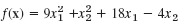
- 19. Minimize f = 2x1 − 10x2 subject to x1 − x2 4, 2x1 + x2 14, x1 + x2 9, −x1 + 3x2 15.
- 20. A factory produces two kinds of gaskets, G1, G2, with net profit of $60 and $30, respectively, Maximize the total daily profit subject to the constraints (xj = number of gaskets Gj produced per day):

SUMMARY OF CHAPTER 22
Unconstrained Optimization. Linear Programming
In optimization problems we maximize or minimize an objective function z = f(x) depending on control variables x1, …, xm whose domain is either unrestricted (“unconstrained optimization,” Sec. 22.1) or restricted by constraints in the form of inequalities or equations or both (“constrained optimization,” Sec. 22.2).
If the objective function is linear and the constraints are linear inequalities in x1, …, xm, then by introducing slack variables xm+1, …, xn we can write the optimization problem in normal form with the objective function given by
![]()
(where cm+1 = … = cn = 0) and the constraints given by
In this case we can then apply the widely used simplex method (Sec. 22.3), a systematic stepwise search through a very much reduced subset of all feasible solutions. Section 22.4 shows how to overcome difficulties with this method.
1GEORGE BERNARD DANTZIG (1914–2005), American mathematician, who is one of the pioneers of linear programming and inventor of the simplex method. According to Dantzig himself (see G. B. Dantzig, Linear programming: The story of how it began, in J. K. Lenestra et al., History of Mathematical Programming: A Collection of Personal Reminiscences. Amsterdam: Elsevier, 1991, pp. 19–31), he was particularly fascinated by Wassilly Leontief's input–output model (Sec. 8.2) and invented his famous method to solve large-scale planning (logistics) problems. Besides Leontief, Dantzig credits others for their pioneering work in linear programming, that is, JOHN VON NEUMANN (1903–1957), Hungarian American mathematician, Institute for Advanced Studies, Princeton University, who made major contributions to game theory, computer science, functional analysis, set theory, quantum mechanics, ergodic theory, and other areas, the Nobel laureates LEONID VITALIYEVICH KANTOROVICH (1912–1986), Russian economist, and TJALLING CHARLES KOOPMANS (1910–1985), Dutch–American economist, who shared the 1975 Nobel Prize in Economics for their contributions to the theory of optimal allocation of resources. Dantzig was a driving force in establishing the field of linear programming and became professor of transportation sciences, operations research, and computer science at Stanford University. For his work see R. W. Cottle (ed.), The Basic George B. Dantzig. Palo Alto, CA: Stanford University Press, 2003.