20. Searching and Sorting

20.1 Introduction

Searching data involves determining whether a value (referred to as the search key) is present in the data and, if so, finding the value’s location. Two popular search algorithms are the simple linear search and the faster, but more complex, binary search. Sorting places data in order, based on one or more sort keys. A list of names could be sorted alphabetically, bank accounts could be sorted by account number, employee payroll records could be sorted by social security number and so on. This chapter introduces two simple sorting algorithms, the selection sort and the insertion sort, along with the more efficient, but more complex, merge sort. Figure 20.1 summarizes the searching and sorting algorithms discussed in this book.

Fig. 20.1. Searching and sorting capabilities in this text.

20.2 Searching Algorithms

Looking up a phone number, accessing a website and checking the definition of a word in a dictionary all involve searching large amounts of data. The next two sections discuss two common search algorithms—one that is easy to program yet relatively inefficient and one that is relatively efficient but more complex to program.

20.2.1 Linear Search

The linear search algorithm searches each element in an array sequentially. If the search key does not match an element in the array, the algorithm tests each element and, when the end of the array is reached, informs the user that the search key is not present. If the search key is in the array, the algorithm tests each element until it finds one that matches the search key and returns the index of that element.

As an example, consider an array containing the following values

34   56   2   10   77   51   93   30   5   52

and a method that is searching for 51. Using the linear search algorithm, the method first checks whether 34 matches the search key. It does not, so the algorithm checks whether 56 matches the search key. The method continues moving through the array sequentially, testing 2, then 10, then 77. When the method tests 51, which matches the search key, the method returns the index 5, which is the location of 51 in the array. If, after checking every array element, the method determines that the search key does not match any element in the array, the method returns a sentinel value (e.g., -1). If there are duplicate values in the array, linear search returns the index of the first element in the array that matches the search key.

Figure 20.2 declares class LinearArray. This class has a private instance variable data (an array of ints), and a static Random object named generator to fill the array with randomly generated ints. When an object of class LinearArray is instantiated, the constructor (lines 12–19) creates and initializes the array data with random ints in the range 10–99.

Fig. 20.2. Class that contains an array of random integers and a method that searches that array sequentially.

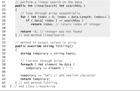
Lines 22–30 perform the linear search. The search key is passed to parameter searchKey. Lines 25–27 loop through the elements in the array. Line 26 compares each element in the array with searchKey. If the values are equal, line 27 returns the index of the element. If the loop ends without finding the value, line 29 returns -1. Lines 33–43 declare method ToString, which returns a string representation of the array for printing.

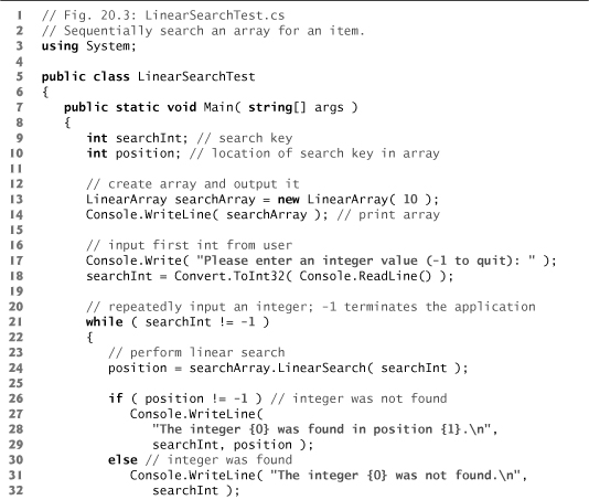
Figure 20.3 creates LinearArray object searchArray containing an array of 10 ints (line 13) and allows the user to search the array for specific elements. Lines 17–18 prompt the user for the search key and store it in searchInt. Lines 21–37 loop until the user enters the sentinel value -1. The array holds ints from 10–99 (line 18 of Fig. 20.2). Line 24 calls the LinearSearch method to determine whether searchInt is in the array. If searchInt is found, LinearSearch returns the position of the element, which the method outputs in lines 27–29. If searchInt is not in the array, LinearSearch returns -1, and the method notifies the user (lines 31–32). Lines 35–36 retrieve the next integer from the user.

Fig. 20.3. Sequentially search an array for an item.

Efficiency of Linear Search

Searching algorithms all accomplish the same goal—finding an element that matches a given search key, if such an element exists. Many things, however, differentiate search algorithms from one another. The major difference is the amount of effort required to complete the search. One way to describe this effort is with Big O notation, which is a measure of the worst-case runtime for an algorithm—that is, how hard an algorithm may have to work to solve a problem. For searching and sorting algorithms, this is particularly dependent on how many elements there are in the data set and the algorithm used.

Suppose an algorithm is designed to test whether the first element of an array is equal to the second element. If the array has 10 elements, this algorithm requires one comparison. If the array has 1,000 elements, this algorithm still requires one comparison. In fact, this algorithm is completely independent of the number of elements in the array, and is thus said to have a constant runtime, which is represented in Big O notation as O(1). An algorithm that is O(1) does not necessarily require only one comparison. O(1) just means that the number of comparisons is constant—it does not grow as the size of the array increases. An algorithm that tests whether the first element of an array is equal to any of the next three elements is still O(1), even though it requires three comparisons.

An algorithm that tests whether the first element of an array is equal to any of the other elements of the array will require at most n – 1 comparisons, where n is the number of elements in the array. If the array has 10 elements, this algorithm requires up to nine comparisons. If the array has 1,000 elements, this algorithm requires up to 999 comparisons. As n grows larger, the n part of the expression “dominates,” and subtracting one becomes inconsequential. Big O is designed to highlight these dominant terms and ignore terms that become unimportant as n grows. For this reason, an algorithm that requires a total of n – 1 comparisons (such as the one we described earlier) is said to be O(n). An O(n) algorithm is referred to as having a linear runtime. O(n) is often pronounced “on the order of n” or more simply “order n.”

Now suppose you have an algorithm that tests whether any element of an array is duplicated elsewhere in the array. The first element must be compared with every other element in the array. The second element must be compared with every other element except the first (it was already compared to the first). The third element must be compared with every other element except the first two. In the end, this algorithm will end up making (n – 1) + (n – 2) + ... + 2 + 1 or n²/2 – n/2 comparisons. As n increases, the n² term dominates and the n term becomes inconsequential. Again, Big O notation highlights the n² term, leaving n²/2. But as we’ll soon see, constant factors are omitted in Big O notation.

Big O is concerned with how an algorithm’s runtime grows in relation to the number of items processed. Suppose an algorithm requires n² comparisons. With four elements, the algorithm will require 16 comparisons; with eight elements, the algorithm will require 64 comparisons. With this algorithm, doubling the number of elements quadruples the number of comparisons. Consider a similar algorithm requiring n²/2 comparisons. With four elements, the algorithm will require eight comparisons; with eight elements, 32 comparisons. Again, doubling the number of elements quadruples the number of comparisons. Both of these algorithms grow as the square of n, so Big O ignores the constant, and both algorithms are considered to be O(n²), referred to as quadratic runtime and pronounced “on the order of n-squared” or more simply “order n-squared.”

When n is small, O(n²) algorithms (running on today’s billions-of-operations-per-second personal computers) will not noticeably affect performance. But as n grows, you’ll start to notice the performance degradation. An O(n²) algorithm running on a million-element array would require a trillion “operations” (where each could actually require several machine instructions to execute). This could require many minutes to execute. A billion-element array would require a quintillion operations, a number so large that the algorithm could take decades! O(n²) algorithms are easy to write, as you’ll see shortly. You’ll also see algorithms with more favorable Big O measures. These efficient algorithms often take more cleverness and effort to create, but their superior performance can be well worth the extra effort, especially as n gets large and algorithms are compounded into larger applications.

The linear search algorithm runs in O(n) time. The worst case in this algorithm is that every element must be checked to determine whether the search item exists in the array. If the size of the array is doubled, the number of comparisons that the algorithm must perform is also doubled. Linear search can provide outstanding performance if the element matching the search key happens to be at or near the front of the array. But we seek algorithms that perform well, on average, across all searches, including those where the element matching the search key is near the end of the array.

Linear search is the easiest search algorithm to program, but it can be slow compared to other search algorithms. If an application needs to perform many searches on large arrays, it may be better to implement a different, more efficient algorithm, such as the binary search, which we present in the next section.

20.2.2 Binary Search

The binary search algorithm is more efficient than the linear search algorithm, but it requires that the array be sorted. The first iteration of this algorithm tests the middle element in the array. If this matches the search key, the algorithm ends. Assuming the array is sorted in ascending order, if the search key is less than the middle element, the search key cannot match any element in the second half of the array and the algorithm continues with only the first half of the array (i.e., the first element up to, but not including, the middle element). If the search key is greater than the middle element, the search key cannot match any element in the first half of the array, and the algorithm continues with only the second half of the array (i.e., the element after the middle element through the last element). Each iteration tests the middle value of the remaining portion of the array, called a subarray. A subarray can have no elements, or it can encompass the entire array. If the search key does not match the element, the algorithm eliminates half of the remaining elements. The algorithm ends by either finding an element that matches the search key or reducing the sub-array to zero size.

As an example, consider the sorted 15-element array

2  3  5  10  27  30  34  51  56  65  77  81  82  93  99

and a search key of 65. An application implementing the binary search algorithm would first check whether 51 is the search key (because 51 is the middle element of the array). The search key (65) is larger than 51, so 51 is “discarded” (i.e., eliminated from consideration) along with the first half of the array (all elements smaller than 51.) Next, the algorithm checks whether 81 (the middle element of the remainder of the array) matches the search key. The search key (65) is smaller than 81, so 81 is discarded along with the elements larger than 81. After just two tests, the algorithm has narrowed the number of values to check to three (56, 65 and 77). The algorithm then checks 65 (which indeed matches the search key) and returns the index of the array element containing 65. This algorithm required just three comparisons to determine whether the search key matched an element of the array. Using a linear search algorithm would have required 10 comparisons. [Note: In this example, we have chosen to use an array with 15 elements so that there will always be an obvious middle element in the array. With an even number of elements, the middle of the array lies between two elements. We implement the algorithm to choose the higher of the two elements.]

Figure 20.4 declares class BinaryArray. This class is similar to LinearArray—it has a private instance variable data (an array of ints), a static Random object named generator to fill the array with randomly generated ints, a constructor, a search method (BinarySearch), a RemainingElements method (which creates a string containing the elements not yet searched) and a ToString method. Lines 12–21 declare the constructor. After initializing the array with random ints from 10–99 (lines 17–18), line 20 calls method Array.Sort on the array data. Method Sort is a static method of class Array that sorts the elements in an array in ascending order. Recall that the binary search algorithm works only on sorted arrays.

Fig. 20.4. Class that contains an array of random integers and a method that uses binary search to find an integer.

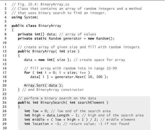
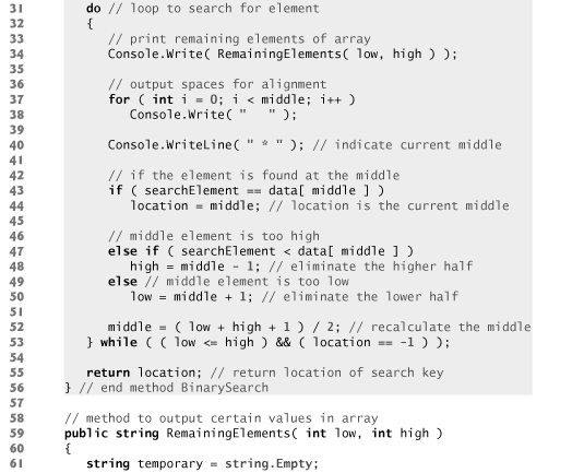
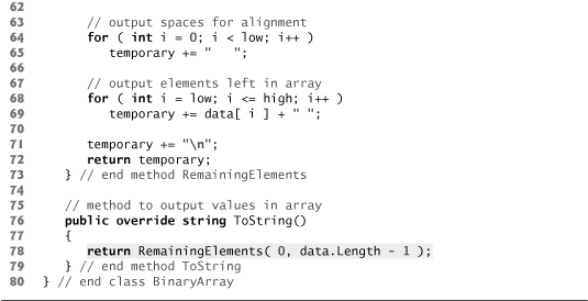
Lines 24–56 declare method BinarySearch. The search key is passed into parameter searchElement (line 24). Lines 26–28 calculate the low end index, high end index and middle index of the portion of the array that the application is currently searching. At the beginning of the method, the low end is 0, the high end is the length of the array minus ¹ and the middle is the average of these two values. Line 29 initializes the location of the element to -1—the value that will be returned if the element is not found. Lines 31–53 loop until low is greater than high (this occurs when the element is not found) or location does not equal -1 (indicating that the search key was found). Line 43 tests whether the value in the middle element is equal to searchElement. If this is true, line 44 assigns middle to location. Then the loop terminates, and location is returned to the caller. Each iteration of the loop tests a single value (line 43) and eliminates half of the remaining values in the array (line 48 or 50).

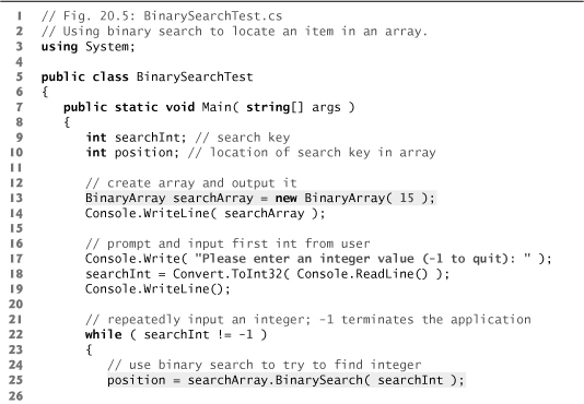
Lines 22–40 of Fig. 20.5 loop until the user enters -1. For each other number the user enters, the application performs a binary search to determine whether the number matches an element in the array. The first line of output from this application is the array of ints, in increasing order. When the user instructs the application to search for 72, the application first tests the middle element (indicated by * in the sample output of Fig. 20.5), which is 52. The search key is greater than 52, so the application eliminates from consideration the first half of the array and tests the middle element from the second half. The search key is smaller than 82, so the application eliminates from consideration the second half of the subarray, leaving only three elements. Finally, the application checks 72 (which matches the search key) and returns the index 9.

Fig. 20.5. Using binary search to locate an item in an array.

Efficiency of Binary Search

In the worst-case scenario, searching a sorted array of 1,023 elements will take only 10 comparisons when using a binary search. Repeatedly dividing 1,023 by 2 (because after each comparison, we are able to eliminate half of the array) and rounding down (because we also remove the middle element) yields the values 511, 255, 127, 63, 31, 15, 7, 3, 1 and 0. The number 1023 (2¹⁰ – 1) is divided by 2 only 10 times to get the value 0, which indicates that there are no more elements to test. Dividing by 2 is equivalent to one comparison in the binary search algorithm. Thus, an array of 1,048,575 (2²⁰ – 1) elements takes a maximum of 20 comparisons to find the key, and an array of one billion elements (which is less than 2³⁰ – 1) takes a maximum of 30 comparisons to find the key. This is a tremendous improvement in performance over the linear search. For a one-billion-element array, this is a difference between an average of 500 million comparisons for the linear search and a maximum of only 30 comparisons for the binary search! The maximum number of comparisons needed for the binary search of any sorted array is the exponent of the first power of 2 greater than the number of elements in the array, which is represented as log₂n. All logarithms grow at roughly the same rate, so in Big O notation the base can be omitted. This results in a big O of O(log n) for a binary search, which is also known as logarithmic runtime.

20.3 Sorting Algorithms

Sorting data (i.e., placing the data in some particular order, such as ascending or descending) is one of the most important computing applications. A bank sorts all checks by account number so that it can prepare individual bank statements at the end of each month. Telephone companies sort their lists of accounts by last name and, further, by first name to make it easy to find phone numbers. Virtually every organization must sort some data—often, massive amounts of it. Sorting data is an intriguing, compute-intensive problem that has attracted substantial research efforts.

It’s important to understand about sorting that the end result—the sorted array—will be the same no matter which (correct) algorithm you use to sort the array. The choice of algorithm affects only the runtime and memory use of the application. The rest of the chapter introduces three common sorting algorithms. The first two—selection sort and insertion sort—are simple to program, but inefficient. The last—merge sort—is much faster than selection sort and insertion sort but more difficult to program. We focus on sorting arrays of simple-type data, namely ints. It’s possible to sort arrays of objects as well—we discuss this in Chapter 23, Collections.

20.3.1 Selection Sort

Selection sort is a simple, but inefficient, sorting algorithm. The first iteration of the algorithm selects the smallest element in the array and swaps it with the first element. The second iteration selects the second-smallest element (which is the smallest of the remaining elements) and swaps it with the second element. The algorithm continues until the last iteration selects the second-largest element and, if necessary, swaps it with the second-to-last element, leaving the largest element in the last position. After the ith iteration, the smallest i elements of the array will be sorted in increasing order in the first i positions of the array.

As an example, consider the array

34   56   4   10   77   51   93   30   5   52

An application that implements selection sort first determines the smallest element (4) of this array, which is contained in index 2 (i.e., position 3). The application swaps 4 with 34, resulting in

4   56   34   10   77   51   93   30   5   52

The application then determines the smallest value of the remaining elements (all elements except 4), which is 5, contained in index 8. The application swaps 5 with 56, resulting in

4   5   34   10   77   51   93   30   56   52

On the third iteration, the application determines the next smallest value (10) and swaps it with 34.

4   5   10   34   77   51   93   30   56   52

The process continues until the array is fully sorted.

4   5   10   30   34   51   52   56   77   93

After the first iteration, the smallest element is in the first position. After the second iteration, the two smallest elements are in order in the first two positions. After the third iteration, the three smallest elements are in order in the first three positions.

Figure 20.6 declares class SelectionSort, which has an instance variable data (an array of ints) and a static Random object generator to generate random integers to fill the array. When an object of class SelectionSort is instantiated, the constructor (lines 12–19) creates and initializes array data with random ints in the range 10–99.

Fig. 20.6. Class that creates an array filled with random integers. Provides a method to sort the array with selection sort.

Lines 22–39 declare the Sort method. Line 24 declares variable smallest, which will store the index of the smallest element in the remaining array. Lines 27–38 loop data.Length - 1 times. Line 29 initializes the index of the smallest element to the current item. Lines 32–34 loop over the remaining elements in the array. For each of these elements, line 33 compares its value to the value of the smallest element. If the current element is smaller than the smallest element, line 34 assigns the current element’s index to smallest. When this loop finishes, smallest will contain the index of the smallest element in the remaining array. Line 36 calls method Swap (lines 42–47) to place the smallest remaining element in the next spot in the array.

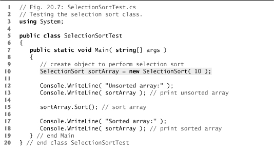
Line 10 of Fig. 20.7 creates a SelectionSort object with 10 elements. Line 13 implicitly calls method ToString to output the unsorted object. Line 15 calls method Sort (lines 22–39 of Fig. 20.6), which sorts the elements using selection sort. Then lines 17–18 output the sorted object. The output uses dashes to indicate the portion of the array that is sorted after each pass (lines 67–68). An asterisk is placed next to the position of the element that was swapped with the smallest element on that pass. On each pass, the element next to the asterisk and the element above the rightmost set of dashes were the two values that were swapped.

Fig. 20.7. Testing the selection sort class.

Efficiency of Selection Sort

The selection sort algorithm runs in O(n²) time. Method Sort in lines 22–39 of Fig. 20.6, which implements the selection sort algorithm, contains nested for loops. The outer for loop (lines 27–38) iterates over the first n – 1 elements in the array, swapping the smallest remaining element to its sorted position. The inner for loop (lines 32–34) iterates over each element in the remaining array, searching for the smallest. This loop executes n – 1 times during the first iteration of the outer loop, n – 2 times during the second iteration, then n– 3, ..., 3, 2, 1. This inner loop will iterate a total of n(n – 1) / 2 or (n² –n)/2. In Big O notation, smaller terms drop out and constants are ignored, leaving a final Big O of O(n²).

20.3.2 Insertion Sort

Insertion sort is another simple, but inefficient, sorting algorithm. Its first iteration takes the second element in the array and, if it’s less than the first, swaps them. The second iteration looks at the third element and inserts it in the correct position with respect to the first two elements, so all three elements are in order. At the ith iteration of this algorithm, the first i elements in the original array will be sorted.

Consider as an example the following array, which is identical to the array used in the discussions of selection sort and merge sort.

34   56   4   10   77   51   93   30   5   52

An application that implements the insertion sort algorithm first looks at the first two elements of the array, 34 and 56. These are already in order, so the application continues (if they were out of order, it would swap them).

In the next iteration, the application looks at the third value, 4. This value is less than 56, so the application stores 4 in a temporary variable and moves 56 one element to the right. The application then checks and determines that 4 is less than 34, so it moves 34 one element to the right. The application has now reached the beginning of the array, so it places 4 in the zeroth position. The array now is

4   34   56   10   77   51   93   30   5   52

In the next iteration, the application stores the value 10 in a temporary variable. Then the application compares 10 to 56 and moves 56 one element to the right because it’s larger than 10. The application then compares 10 to 34, moving 34 one element to the right. When the application compares 10 to 4, it observes that 10 is larger than 4 and places 10 in element 1. The array now is

4   10   34   56   77   51   93   30   5   52

Using this algorithm, at the ith iteration, the original array’s first i elements are sorted, but they may not be in their final locations—smaller values may be located later in the array.

Figure 20.8 declares the InsertionSort class. Lines 22–46 declare the Sort method. Line 24 declares variable insert, which holds the element to be inserted while the other elements are moved. Lines 27–45 loop through data.Length - 1 items in the array. In each iteration, line 30 stores in variable insert the value of the element that will be inserted in the sorted portion of the array. Line 33 declares and initializes variable moveItem, which keeps track of where to insert the element. Lines 36–41 loop to locate the correct position to insert the element. The loop will terminate either when the application reaches the front of the array or when it reaches an element that is less than the value to be inserted. Line 39 moves an element to the right, and line 40 decrements the position at which to insert the next element. After the loop ends, line 43 inserts the element in place. Figure 20.9 is the same as Fig. 20.7 except that it creates and uses an InsertionSort object. The output of this application uses dashes to indicate the portion of the array that is sorted after each pass (lines 66–67 of Fig. 20.8). An asterisk is placed next to the element that was inserted in place on that pass.

Fig. 20.8. Class that creates an array filled with random integers. Provides a method to sort the array with insertion sort.

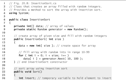
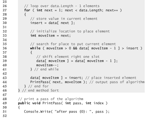
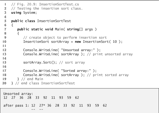
Fig. 20.9. Testing the insertion sort class.

Efficiency of Insertion Sort

The insertion sort algorithm also runs in O(n²) time. Like selection sort, the implementation of insertion sort (lines 22–46 of Fig. 20.8) contains nested loops. The for loop (lines 27–45) iterates data.Length - 1 times, inserting an element in the appropriate position in the elements sorted so far. For the purposes of this application, data.Length - 1 is equivalent to n – 1 (as data.Length is the size of the array). The while loop (lines 36–41) iterates over the preceding elements in the array. In the worst case, this while loop will require n – 1 comparisons. Each individual loop runs in O(n) time. In Big O notation, nested loops mean that you must multiply the number of iterations of each loop. For each iteration of an outer loop, there will be a certain number of iterations of the inner loop. In this algorithm, for each O(n) iterations of the outer loop, there will be O(n) iterations of the inner loop. Multiplying these values results in a Big O of O(n²).

20.3.3 Merge Sort

Merge sort is an efficient sorting algorithm but is conceptually more complex than selection sort and insertion sort. The merge sort algorithm sorts an array by splitting it into two equal-sized subarrays, sorting each subarray and merging them in one larger array. With an odd number of elements, the algorithm creates the two subarrays such that one has one more element than the other.

The implementation of merge sort in this example is recursive. The base case is an array with one element. A one-element array is, of course, sorted, so merge sort immediately returns when it’s called with a one-element array. The recursion step splits an array in two approximately equal-length pieces, recursively sorts them and merges the two sorted arrays in one larger, sorted array.

Suppose the algorithm has already merged smaller arrays to create sorted arrays A:

4   10   34   56   77

and B:

5   30   51   52   93

Merge sort combines these two arrays in one larger, sorted array. The smallest element in A is 4 (located in the zeroth element of A). The smallest element in B is 5 (located in the zeroth element of B). In order to determine the smallest element in the larger array, the algorithm compares 4 and 5. The value from A is smaller, so 4 becomes the first element in the merged array. The algorithm continues by comparing 10 (the second element in A) to 5 (the first element in B). The value from B is smaller, so 5 becomes the second element in the larger array. The algorithm continues by comparing 10 to 30, with 10 becoming the third element in the array, and so on.

Lines 22–25 of Fig. 20.10 declare the Sort method. Line 24 calls method SortArray with 0 and data.Length - 1 as the arguments—these are the beginning and ending indices of the array to be sorted. These values tell method SortArray to operate on the entire array.

Fig. 20.10. Class that creates an array filled with random integers. Provides a method to sort the array with merge sort.

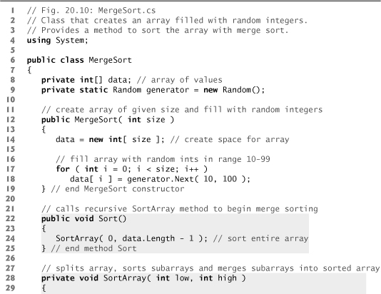
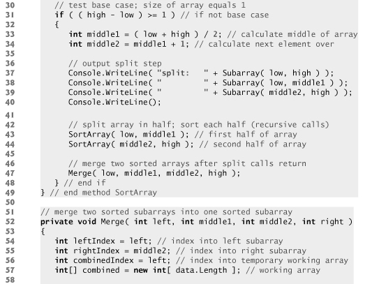
Method SortArray is declared in lines 28–49. Line 31 tests the base case. If the size of the array is 1, the array is already sorted, so the method simply returns immediately. If the size of the array is greater than 1, the method splits the array in two, recursively calls method SortArray to sort the two subarrays and merges them. Line 43 recursively calls method SortArray on the first half of the array, and line 44 recursively calls method Sort-Array on the second half of the array. When these two method calls return, each half of the array has been sorted. Line 47 calls method Merge (lines 52–91) on the two halves of the array to combine the two sorted arrays in one larger sorted array.

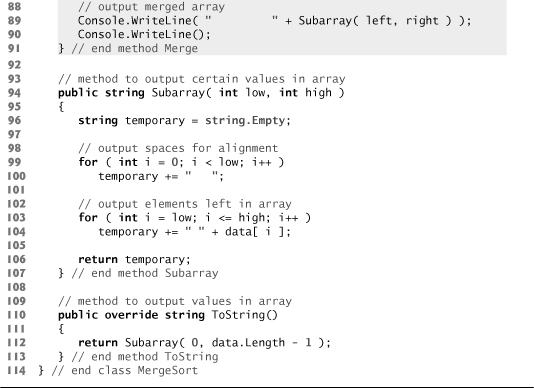
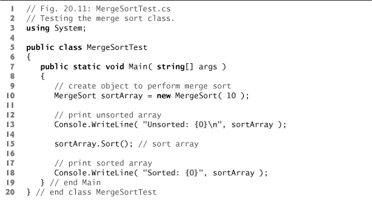
Lines 64–72 in method Merge loop until the application reaches the end of either sub-array. Line 68 tests which element at the beginning of the arrays is smaller. If the element in the left array is smaller or equal, line 69 places it in position in the combined array. If the element in the right array is smaller, line 71 places it in position in the combined array. When the while loop has completed (line 72), one entire subarray is placed in the combined array, but the other subarray still contains data. Line 75 tests whether the left array has reached the end. If so, lines 77–78 fill the combined array with the remaining elements of the right array. If the left array has not reached the end, then the right array has, and lines 81–82 fill the combined array with the remaining elements of the left array. Finally, lines 85–86 copy the combined array into the original array. Figure 20.11 creates and uses a MergeSort object. The output from this application displays the splits and merges performed by merge sort, showing the progress of the sort at each step of the algorithm.

Fig. 20.11. Testing the merge sort class.

Efficiency of Merge Sort

Merge sort is a far more efficient algorithm than either insertion sort or selection sort when sorting large sets of data. Consider the first (nonrecursive) call to method SortArray. This results in two recursive calls to method SortArray with subarrays each approximately half the size of the original array, and a single call to method Merge. This call to method Merge requires, at worst, n – 1 comparisons to fill the original array, which is O(n). (Recall that each element in the array can be chosen by comparing one element from each of the subar-rays.) The two calls to method SortArray result in four more recursive calls to SortArray, each with a subarray approximately a quarter the size of the original array, along with two calls to method Merge. These two calls to method Merge each require, at worst, n/2 – 1 comparisons for a total number of comparisons of (n/2 – 1) + (n/2 – 1) = n – 2, which is O(n). This process continues, each call to SortArray generating two additional calls to method SortArray and a call to Merge, until the algorithm has split the array into one-element subarrays. At each level, O(n) comparisons are required to merge the subarrays. Each level splits the size of the arrays in half, so doubling the size of the array requires only one more level. Quadrupling the size of the array requires only two more levels. This pattern is logarithmic and results in log₂n levels. This results in a total efficiency of O(n log n).

20.4 Summary of the Efficiency of Searching and Sorting Algorithms

Figure 20.12 summarizes many of the searching and sorting algorithms covered in this book and lists the Big O of each. Figure 20.13 lists the Big O values covered in this chapter, along with a number of values for n to highlight the differences in the growth rates.

Fig. 20.12. Searching and sorting algorithms with Big O values.

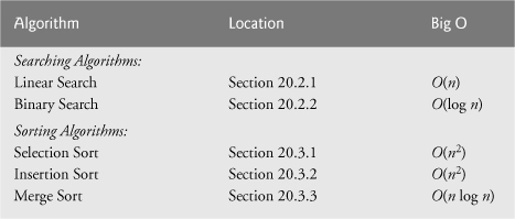
Fig. 20.13. Number of comparisons for common Big O notations.

20.5 Wrap-Up

In this chapter, you learned how to search for items in arrays and how to sort arrays so that their elements are arranged in order. We discussed linear search and binary search, and selection sort, insertion sort and merge sort. You learned that linear search can operate on any set of data, but that binary search requires the data to be sorted first. You also learned that the simplest searching and sorting algorithms can exhibit poor performance. We introduced Big O notation—a measure of the efficiency of algorithms—and used it to compare the efficiency of the algorithms we discussed. In the next chapter, you’ll learn about dynamic data structures that can grow or shrink at execution time.