21. Data Structures

21.1 Introduction

This chapter continues our four-chapter treatment of data structures. Most of the data structures that we have studied thus far have had fixed sizes, such as one- and two-dimensional arrays. Previously, we also introduced the dynamically resizable List<T> collection (Chapter 9). This chapter enhances our discussion of dynamic data structures that grow and shrink at execution time. Linked lists are collections of data items “lined up in a row” or “chained together”—users can make insertions and deletions anywhere in a linked list. Stacks are important in compilers and operating systems; insertions and deletions are made at only one end—its top. Queues represent waiting lines; insertions are made at the back (also referred to as the tail) of a queue, and deletions are made from the front (also referred to as the head) of a queue. Binary trees facilitate high-speed searching and sorting of data, efficient elimination of duplicate data items, representation of file-system directories and compilation of expressions into machine language. These data structures have many other interesting applications as well.

We’ll discuss each of these major types of data structures and implement programs that create and manipulate them. We use classes, inheritance and composition to create and package these data structures for reusability and maintainability. In Chapter 22, we introduce generics, which allow you to declare data structures that can be automatically adapted to contain data of any type. In Chapter 23, we discuss C#’s predefined collection classes that implement various data structures.

The chapter examples are practical programs that will be useful in more advanced courses and in industrial applications. The programs focus on reference manipulation.

21.2 Simple-Type structs, Boxing and Unboxing

The data structures we discuss in this chapter store object references. However, as you’ll soon see, we’re able to store both simple- and reference-type values in these data structures. This section discusses the mechanisms that enable simple-type values to be manipulated as objects.

Simple-Type structs

Each simple type (see Appendix B, Simple Types) has a corresponding struct in namespace System that declares the simple type. These structs are called Boolean, Byte, SByte, Char, Decimal, Double, Single, Int32, UInt32, Int64, UInt64, Int16 and UInt16. Types declared with keyword struct are implicitly value types.

Simple types are actually aliases for their corresponding structs, so a variable of a simple type can be declared using either the keyword for that simple type or the struct name—e.g., int and Int32 are interchangeable. The methods related to a simple type are located in the corresponding struct (e.g., method Parse, which converts a string to an int value, is located in struct Int32). Refer to the documentation for the corresponding struct type to see the methods available for manipulating values of that type.

Boxing and Unboxing Conversions

Simple types and other structs inherit from class ValueType in namespace System. Class ValueType inherits from class object. Thus, any simple-type value can be assigned to an object variable; this is referred to as a boxing conversion and enables simple types to be used anywhere objects are expected. In a boxing conversion, the simple-type value is copied into an object so that the simple-type value can be manipulated as an object. Boxing conversions can be performed either explicitly or implicitly as shown in the following statements:

int i = 5; // create an int value
object object1 = ( object ) i; // explicitly box the int value
object object2 = i; // implicitly box the int value

After executing the preceding code, both object1 and object2 refer to two different objects that contain a copy of the integer value in int variable i.

An unboxing conversion can be used to explicitly convert an object reference to a simple value, as shown in the following statement:

int int1 = ( int ) object1; // explicitly unbox the int value

Explicitly attempting to unbox an object reference that does not refer to the correct simple value type causes an InvalidCastException.

In Chapters 22 and 23, we discuss C#’s generics and generic collections. As you’ll see, generics eliminate the overhead of boxing and unboxing conversions by enabling us to create and use collections of specific value types.

21.3 Self-Referential Classes

A self-referential class contains a reference member that refers to an object of the same class type. For example, the class declaration in Fig. 21.1 defines the shell of a self-referential class named Node. This type has two properties—integer Data and Node reference Next. Next references an object of type Node, an object of the same type as the one being declared here—hence, the term “self-referential class.” Next is referred to as a link (i.e., Next can be used to “tie” an object of type Node to another object of the same type).

Fig. 21.1. Self-referential Node class declaration.

Self-referential objects can be linked together to form useful data structures, such as lists, queues, stacks and trees. Figure 21.2 illustrates two self-referential objects linked together to form a linked list. A backslash (representing a null reference) is placed in the link member of the second self-referential object to indicate that the link does not refer to another object. The backslash is for illustration purposes; it does not correspond to the backslash character in C#. A null link normally indicates the end of a data structure.

Fig. 21.2. Self-referential class objects linked together.

Creating and maintaining dynamic data structures requires dynamic memory allocation—a program’s ability to obtain more memory space at execution time to hold new nodes and to release space no longer needed. As you learned in Section 10.9, C# programs do not explicitly release dynamically allocated memory—rather, the CLR performs automatic garbage collection.

The new operator is essential to dynamic memory allocation. Operator new takes as an operand the type of the object being dynamically allocated and returns a reference to an object of that type. For example, the statement

Node nodeToAdd = new Node( 10 );

allocates the appropriate amount of memory to store a Node and stores a reference to this object in nodeToAdd. If no memory is available, new throws an OutOfMemoryException. The constructor argument 10 specifies the Node object’s data.

The following sections discuss lists, stacks, queues and trees. These data structures are created and maintained with dynamic memory allocation and self-referential classes.

21.4 Linked Lists

A linked list is a linear collection (i.e., a sequence) of self-referential class objects, called nodes, connected by reference links—hence, the term “linked” list. A program accesses a linked list via a reference to the first node of the list. Each subsequent node is accessed via the link-reference member stored in the previous node. By convention, the link reference in the last node of a list is set to null to mark the end of the list. Data is stored in a linked list dynamically—that is, each node is created as necessary. A node can contain data of any type, including references to objects of other classes. Stacks and queues are also linear data structures—in fact, they’re constrained versions of linked lists. Trees are nonlinear data structures.

Lists of data can be stored in arrays, but linked lists provide several advantages. A linked list is appropriate when the number of data elements to be represented in the data structure is unpredictable. Unlike a linked list, the size of a conventional C# array cannot be altered, because the array size is fixed at creation time. Conventional arrays can become full, but linked lists become full only when the system has insufficient memory to satisfy dynamic memory allocation requests.

Programmers can maintain linked lists in sorted order simply by inserting each new element at the proper point in the list (locating the proper insertion point does take time). They do not need to move existing list elements.

Normally linked-list nodes are not stored contiguously in memory. Rather, the nodes are logically contiguous. Figure 21.3 illustrates a linked list with several nodes.

Fig. 21.3. Linked list graphical representation.

Linked-List Implementation

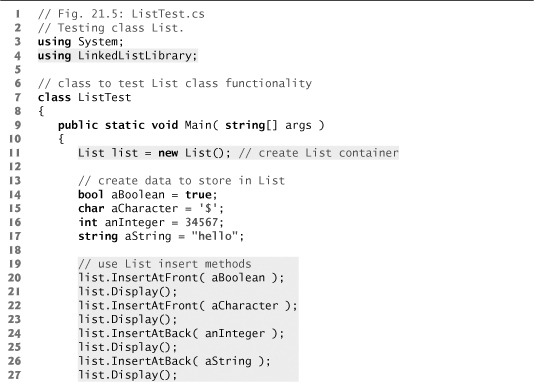
Figures 21.4–21.5 use an object of our List class to manipulate a list of miscellaneous object types. Class ListTest’s Main method (Fig. 21.5) creates a list of objects, inserts objects at the beginning of the list using List method InsertAtFront, inserts objects at the end of the list using List method InsertAtBack, deletes objects from the front of the list using List method RemoveFromFront and deletes objects from the end of the list using List method Remove-FromBack. After each insert and delete operation, the program invokes List method Display to output the current list contents. If an attempt is made to remove an item from an empty list, an EmptyListException occurs. A detailed discussion of the program follows.

The program consists of four classes—ListNode (Fig. 21.4, lines 8–30), List (lines 33–147), EmptyListException (lines 150–172) and ListTest (Fig. 21.5). The classes in Fig. 21.4 create a linked-list library (defined in namespace LinkedListLibrary) that can be reused throughout this chapter. You should place the code of Fig. 21.4 in its own class library project, as we described in Section 15.13.

Fig. 21.4. ListNode, List and EmptyListException class declarations.

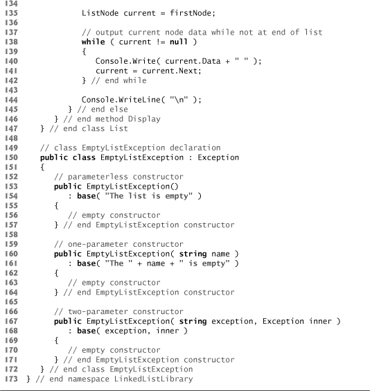
Class ListNode

Encapsulated in each List object is a linked list of ListNode objects. Class ListNode (Fig. 21.4, lines 8–30) contains two properties—Data and Next. Data can refer to any object. [Note: Typically, a data structure will contain data of only one type, or data of any type derived from one base type.] In this example, we use data of various types derived from object to demonstrate that our List class can store data of any type. Next stores a reference to the next ListNode object in the linked list. The ListNode constructors (lines 18–21 and 25–29) enable us to initialize a ListNode that will be placed at the end of a List or before a specific ListNode in a List, respectively.

Class List

Class List (lines 33–147) contains private instance variables firstNode (a reference to the first ListNode in a List) and lastNode (a reference to the last ListNode in a List). The constructors (lines 40–44 and 47–50) initialize both references to null and enable us to specify the List’s name for output purposes. InsertAtFront (lines 55–61), InsertAt-Back (lines 66–72), RemoveFromFront (lines 75–89) and RemoveFromBack (lines 92–116) are the primary methods of class List. Method IsEmpty (lines 119–122) is a predicate method that determines whether the list is empty (i.e., the reference to the first node of the list is null). Predicate methods typically test a condition and do not modify the object on which they’re called. If the list is empty, method IsEmpty returns true; otherwise, it returns false. Method Display (lines 125–146) displays the list’s contents. A detailed discussion of class List’s methods follows Fig. 21.5.

Class EmptyListException

Class EmptyListException (lines 150–172) defines an exception class that we use to indicate illegal operations on an empty List.

Class ListTest

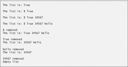
Class ListTest (Fig. 21.5) uses the linked-list library to create and manipulate a linked list. [Note: In the project containing Fig. 21.5, you must add a reference to the class library containing the classes in Fig. 21.4. If you use our existing example, you may need to update this reference.] Line 11 creates a new List object and assigns it to variable list. Lines 14–17 create data to add to the list. Lines 20–27 use List insertion methods to insert these values and use List method Display to output the contents of list after each insertion. The values of the simple-type variables are implicitly boxed in lines 20, 22 and 24 where object references are expected. The code inside the try block (lines 33–50) removes objects via List deletion methods, outputs each removed object and outputs list after every deletion. If there’s an attempt to remove an object from an empty list, the catch at lines 51–54 catches the EmptyListException and displays an error message.

Fig. 21.5. Testing class List.

Method InsertAtFront

Over the next several pages, we discuss each of the methods of class List in detail. Method InsertAtFront (Fig. 21.4, lines 55–61) places a new node at the front of the list. The method consists of three steps:

1. Call IsEmpty to determine whether the list is empty (line 57).
2. If the list is empty, set both firstNode and lastNode to refer to a new ListNode initialized with insertItem (line 58). The ListNode constructor at lines 18–21 of Fig. 21.4 calls the ListNode constructor at lines 25–29, which sets property Data to refer to the object passed as the first argument and sets the Next property’s reference to null.
3. If the list is not empty, the new node is “linked” into the list by setting firstNode to refer to a new ListNode object initialized with insertItem and firstNode (line 60). When the ListNode constructor (lines 25–29) executes, it sets property Data to refer to the object passed as the first argument and performs the insertion by setting the Next reference to the ListNode passed as the second argument.

In Fig. 21.6, part (a) shows a list and a new node during the InsertAtFront operation before the new node is linked into the list. The dashed lines and arrows in part (b) illustrate Step 3 of the InsertAtFront operation, which enables the node containing 12 to become the new list front.

Fig. 21.6. InsertAtFront operation.

Method InsertAtBack

Method InsertAtBack (Fig. 21.4, lines 66–72) places a new node at the back of the list. The method consists of three steps:

1. Call IsEmpty to determine whether the list is empty (line 68).
2. If the list is empty, set both firstNode and lastNode to refer to a new ListNode initialized with insertItem (lines 68–69). The ListNode constructor at lines 18–21 calls the ListNode constructor at lines 25–29, which sets property Data to refer to the object passed as the first argument and sets the Next reference to null.
3. If the list is not empty, link the new node into the list by setting lastNode and lastNode.Next to refer to a new ListNode object initialized with insertItem (line 71). When the ListNode constructor (lines 18–21) executes, it calls the constructor at lines 25–29, which sets property Data to refer to the object passed as an argument and sets the Next reference to null.

In Fig. 21.7, part (a) shows a list and a new node during the InsertAtBack operation before the new node has been linked into the list. The dashed lines and arrows in part (b) illustrate Step 3 of method InsertAtBack, which enables a new node to be added to the end of a list that is not empty.

Fig. 21.7. InsertAtBack operation.

Method RemoveFromFront

Method RemoveFromFront (Fig. 21.4, lines 75–89) removes the front node of the list and returns a reference to the removed data. The method throws an EmptyListException (line 78) if the programmer tries to remove a node from an empty list. Otherwise, the method returns a reference to the removed data. After determining that a List is not empty, the method consists of four steps to remove the first node:

1. Assign firstNode.Data (the data being removed from the list) to variable removeItem (line 80).
2. If the objects to which firstNode and lastNode refer are the same object, the list has only one element, so the method sets firstNode and lastNode to null (line 84) to remove the node from the list (leaving the list empty).
3. If the list has more than one node, the method leaves reference lastNode as is and assigns firstNode.Next to firstNode (line 86). Thus, firstNode references the node that was previously the second node in the List.
4. Return the removeItem reference (line 88).

In Fig. 21.8, part (a) illustrates a list before a removal operation. The dashed lines and arrows in part (b) show the reference manipulations.

Fig. 21.8. RemoveFromFront operation.

Method RemoveFromBack

Method RemoveFromBack (Fig. 21.4, lines 92–116) removes the last node of a list and returns a reference to the removed data. The method throws an EmptyListException (line 95) if the program attempts to remove a node from an empty list. The method consists of several steps:

1. Assign lastNode.Data (the data being removed from the list) to variable removeItem (line 97).
2. If firstNode and lastNode refer to the same object (line 100), the list has only one element, so the method sets firstNode and lastNode to null (line 101) to remove that node from the list (leaving the list empty).
3. If the list has more than one node, create ListNode variable current and assign it firstNode (line 104).
4. Now “walk the list” with current until it references the node before the last node. The while loop (lines 107–108) assigns current.Next to current as long as current.Next is not equal to lastNode.
5. After locating the second-to-last node, assign current to lastNode (line 111) to update which node is last in the list.
6. Set current.Next to null (line 112) to remove the last node from the list and terminate the list at the current node.
7. Return the removeItem reference (line 115).

In Fig. 21.9, part (a) illustrates a list before a removal operation. The dashed lines and arrows in part (b) show the reference manipulations.

Fig. 21.9. RemoveFromBack operation.

Method Display

Method Display (Fig. 21.4, lines 125–146) first determines whether the list is empty (line 127). If so, Display displays a string consisting of the string "Empty " and the list’s name, then returns control to the calling method. Otherwise, Display outputs the data in the list. The method writes a string consisting of the string "The ", the list’s name and the string "is: ". Then line 135 creates ListNode variable current and initializes it with firstNode. While current is not null, there are more items in the list. Therefore, the method displays current.Data (line 140), then assigns current.Next to current (line 141) to move to the next node in the list.

Linear and Circular Singly Linked and Doubly Linked Lists

The kind of linked list we have been discussing is a singly linked list—it begins with a reference to the first node, and each node contains a reference to the next node “in sequence.” This list terminates with a node whose reference member has the value null. A singly linked list may be traversed in only one direction.

A circular, singly linked list (Fig. 21.10) begins with a reference to the first node, and each node contains a reference to the next node. The “last node” does not contain a null reference; rather, the reference in the last node points back to the first node, thus closing the “circle.”

Fig. 21.10. Circular, singly linked list.

A doubly linked list (Fig. 21.11) allows traversals both forward and backward. Such a list is often implemented with two “start references”—one that refers to the first element of the list to allow front-to-back traversal of the list and one that refers to the last element to allow back-to-front traversal. Each node has both a forward reference to the next node in the list and a backward reference to the previous node. If your list contains an alphabetized telephone directory, for example, a search for someone whose name begins with a letter near the front of the alphabet might begin from the front of the list. A search for someone whose name begins with a letter near the end of the alphabet might begin from the back.

Fig. 21.11. Doubly linked list.

In a circular, doubly linked list (Fig. 21.12), the forward reference of the last node refers to the first node, and the backward reference of the first node refers to the last node, thus closing the “circle.”

Fig. 21.12. Circular, doubly linked list.

21.5 Stacks

A stack is a constrained version of a linked list—it receives new nodes and releases nodes only at the top. For this reason, a stack is referred to as a last-in, first-out (LIFO) data structure.

The primary operations to manipulate a stack are push and pop. Operation push adds a new node to the top of the stack. Operation pop removes a node from the top of the stack and returns the data item from the popped node.

Stacks have many interesting applications. For example, when a program calls a method, the called method must know how to return to its caller, so the return address is pushed onto the method-call stack. If a series of method calls occurs, the successive return values are pushed onto the stack in last-in, first-out order so that each method can return to its caller. Stacks support recursive method calls in the same manner that they do conventional nonrecursive method calls.

The System.Collections namespace contains class Stack for implementing and manipulating stacks that can grow and shrink during program execution.

In our next example, we take advantage of the close relationship between lists and stacks to implement a stack class by reusing a list class. We demonstrate two different forms of reusability. First, we implement the stack class by inheriting from class List of Fig. 21.4. Then we implement an identically performing stack class through composition by including a List object as a private member of a stack class.

Stack Class That Inherits from List

The program of Figs. 21.13 and 21.14 creates a stack class by inheriting from class List of Fig. 21.4 (line 8 of Fig. 21.3). We want the stack to have methods Push, Pop, IsEmpty and Display. Essentially, these are the methods InsertAtFront, RemoveFromFront, IsEmpty and Display of class List. Of course, class List contains other methods (such as InsertAtBack and RemoveFromBack) that we would rather not make accessible through the public interface of the stack. It is important to remember that all methods in the public interface of class List are also public methods of the derived class StackInheritance (Fig. 21.13).

Fig. 21.13. Implementing a stack by inheriting from class List.

The implementation of each StackInheritance method calls the appropriate List method—method Push calls InsertAtFront, method Pop calls RemoveFromFront. Class StackInheritance does not define methods IsEmpty and Display, because StackInheritance inherits these methods from class List into StackInheritance’s public interface. Class StackInheritance uses namespace LinkedListLibrary (Fig. 21.4); thus, the class library that defines StackInheritance must have a reference to the LinkedListLibrary class library.

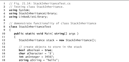
StackInheritanceTest’s Main method (Fig. 21.14) uses class StackInheritance to create a stack of objects called stack (line 12). Lines 15–18 define four values that will be pushed onto the stack and popped off it. The program pushes onto the stack (lines 21, 23, 25 and 27) a bool containing true, a char containing '$', an int containing 34567 and a string containing "hello". An infinite while loop (lines 33–38) pops the elements from the stack. When the stack is empty, method Pop throws an EmptyListException, and the program displays the exception’s stack trace, which shows the program-execution stack at the time the exception occurred. The program uses method Display (inherited by StackInheritance from class List) to output the contents of the stack after each operation. Class StackInheritanceTest uses namespace LinkedListLibrary (Fig. 21.4) and namespace StackInheritanceLibrary (Fig. 21.13); thus, the solution for class StackInheritanceTest must have references to both class libraries.

Fig. 21.14. Testing class StackInheritance.

Stack Class That Contains a Reference to a List

Another way to implement a stack class is by reusing a list class through composition. The class in Fig. 21.15 uses a private object of class List (line 10) in the declaration of class StackComposition. Composition enables us to hide the methods of class List that should not be in our stack’s public interface by providing public interface methods only to the required List methods. This class implements each stack method by delegating its work to an appropriate List method. StackComposition’s methods call List methods Insert-AtFront, RemoveFromFront, IsEmpty and Display. In this example, we do not show class StackCompositionTest, because the only difference in this example is that we change the name of the stack class from StackInheritance to StackComposition.

Fig. 21.15. StackComposition class encapsulates functionality of class List.

21.6 Queues

Another commonly used data structure is the queue. A queue is similar to a checkout line in a supermarket—the cashier services the person at the beginning of the line first. Other customers enter the line only at the end and wait for service. Queue nodes are removed only from the head (or front) of the queue and are inserted only at the tail (or end). For this reason, a queue is a first-in, first-out (FIFO) data structure. The insert and remove operations are known as enqueue and dequeue.

Queues have many uses in computer systems. Computers with only a single processor can service only one application at a time. Each application requiring processor time is placed in a queue. The application at the front of the queue is the next to receive service. Each application gradually advances to the front as the applications before it receive service.

Queues are also used to support print spooling. For example, a single printer might be shared by all users of a network. Many users can send print jobs to the printer, even when the printer is already busy. These print jobs are placed in a queue until the printer becomes available. A program called a spooler manages the queue to ensure that as each print job completes, the next one is sent to the printer.

Information packets also wait in queues in computer networks. Each time a packet arrives at a network node, it must be routed to the next node along the path to the packet’s final destination. The routing node routes one packet at a time, so additional packets are enqueued until the router can route them.

A file server in a computer network handles file-access requests from many clients throughout the network. Servers have a limited capacity to service requests from clients. When that capacity is exceeded, client requests wait in queues.

Queue Class That Inherits from List

The program of Figs. 21.16 and 21.17 creates a queue class by inheriting from a list class. We want the QueueInheritance class (Fig. 21.16) to have methods Enqueue, Dequeue, IsEmpty and Display. Essentially, these are the methods InsertAtBack, RemoveFrom-Front, IsEmpty and Display of class List. Of course, the list class contains other methods (such as InsertAtFront and RemoveFromBack) that we would rather not make accessible through the public interface to the queue class. Remember that all methods in the public interface of the List class are also public methods of the derived class QueueInheritance.

Fig. 21.16. Implementing a queue by inheriting from class List.

Fig. 21.17. Testing class QueueInheritance.

The implementation of each QueueInheritance method calls the appropriate List method—method Enqueue calls InsertAtBack and method Dequeue calls RemoveFrom-Front. Calls to IsEmpty and Display invoke the base-class versions that were inherited from class List into QueueInheritance’s public interface. Class QueueInheritance uses namespace LinkedListLibrary (Fig. 21.4); thus, the class library for QueueInheritance must have a reference to the LinkedListLibrary class library.

Class QueueInheritanceTest’s Main method (Fig. 21.17) creates a QueueInheritance object called queue. Lines 15–18 define four values that will be enqueued and dequeued. The program enqueues (lines 21, 23, 25 and 27) a bool containing true, a char containing '$', an int containing 34567 and a string containing "hello". Class QueueInheritanceTest uses namespace LinkedListLibrary and namespace QueueInheritanceLibrary; thus, the solution for class StackInheritanceTest must have references to both class libraries.

An infinite while loop (lines 36–41) dequeues the elements from the queue in FIFO order. When there are no objects left to dequeue, method Dequeue throws an Empty-ListException, and the program displays the exception’s stack trace, which shows the program-execution stack at the time the exception occurred. The program uses method Display (inherited from class List) to output the contents of the queue after each operation. Class QueueInheritanceTest uses namespace LinkedListLibrary (Fig. 21.4) and namespace QueueInheritanceLibrary (Fig. 21.16); thus, the solution for class QueueInheritanceTest must have references to both class libraries.

21.7 Trees

Linked lists, stacks and queues are linear data structures (i.e., sequences). A tree is a nonlinear, two-dimensional data structure with special properties. Tree nodes contain two or more links.

Basic Terminology

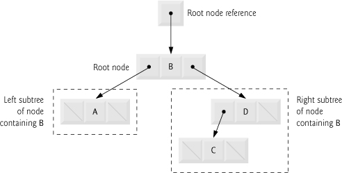
With binary trees (Fig. 21.18), each tree node contains two links (none, one or both of which may be null). The root node is the first node in a tree. Each link in the root node refers to a child. The left child is the first node in the left subtree, and the right child is the first node in the right subtree. The children of a specific node are called siblings. A node with no children is called a leaf node. Computer scientists normally draw trees from the root node down—exactly the opposite of the way most trees grow in nature.

Fig. 21.18. Binary-tree graphical representation.

Binary Search Trees

In our binary-tree example, we create a special binary tree called a binary search tree. A binary search tree (with no duplicate node values) has the characteristic that the values in any left subtree are less than the value in the subtree’s parent node, and the values in any right subtree are greater than the value in the subtree’s parent node. Figure 21.19 illustrates a binary search tree with 9 integer values. The shape of the binary search tree that corresponds to a set of data can depend on the order in which the values are inserted into the tree.

Fig. 21.19. Binary search tree containing 9 values.

21.7.1 Binary Search Tree of Integer Values

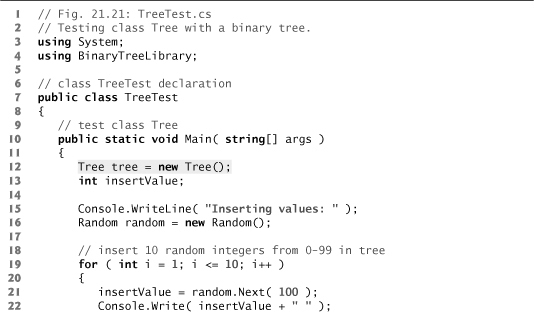
The application of Figs. 21.20 and 21.21 creates a binary search tree of integers and traverses it (i.e., walks through all its nodes) in three ways—using recursive inorder, preorder and postorder traversals. The program generates 10 random numbers and inserts each into the tree. Figure 21.20 defines class Tree in namespace BinaryTreeLibrary for reuse purposes. Figure 21.21 defines class TreeTest to demonstrate class Tree’s functionality. Method Main of class TreeTest instantiates an empty Tree object, then randomly generates 10 integers and inserts each value in the binary tree by calling Tree method Insert-Node. The program then performs preorder, inorder and postorder traversals of the tree. We’ll discuss these traversals shortly.

Fig. 21.20. Declaration of class TreeNode and class Tree.

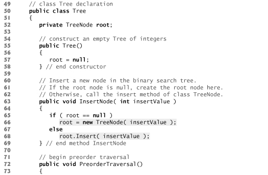
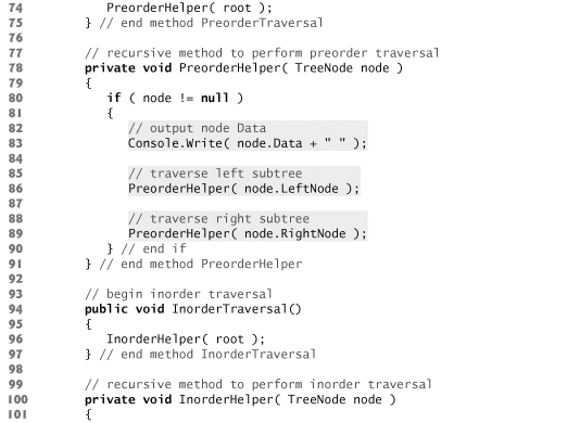
Fig. 21.21. Testing class Tree with a binary tree.

Class TreeNode (lines 8–47 of Fig. 21.20) is a self-referential class containing three properties—LeftNode and RightNode of type TreeNode and Data of type int. Initially, every TreeNode is a leaf node, so the constructor (lines 20–24) initializes references Left-Node and RightNode to null. We discuss TreeNode method Insert (lines 28–46) shortly.

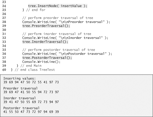
Class Tree (lines 50–136 of Fig. 21.20) manipulates objects of class TreeNode. Class Tree has as private data root (line 52)—a reference to the root node of the tree. The class contains public method InsertNode (lines 63–69) to insert a new node in the tree and public methods PreorderTraversal (lines 72–75), InorderTraversal (lines 94–97) and PostorderTraversal (lines 116–119) to begin traversals of the tree. Each of these methods calls a separate recursive utility method to perform the traversal operations on the internal representation of the tree. The Tree constructor (lines 55–58) initializes root to null to indicate that the tree initially is empty.

Tree method InsertNode (lines 63–69) first determines whether the tree is empty. If so, line 66 allocates a new TreeNode, initializes the node with the integer being inserted in the tree and assigns the new node to root. If the tree is not empty, InsertNode calls TreeNode method Insert (lines 28–46), which recursively determines the location for the new node in the tree and inserts the node at that location. A node can be inserted only as a leaf node in a binary search tree.

The TreeNode method Insert compares the value to insert with the data value in the root node. If the insert value is less than the root-node data, the program determines whether the left subtree is empty (line 33). If so, line 34 allocates a new TreeNode, initializes it with the integer being inserted and assigns the new node to reference LeftNode. Otherwise, line 36 recursively calls Insert for the left subtree to insert the value into the left subtree. If the insert value is greater than the root-node data, the program determines whether the right subtree is empty (line 41). If so, line 42 allocates a new TreeNode, initializes it with the integer being inserted and assigns the new node to reference RightNode. Otherwise, line 44 recursively calls Insert for the right subtree to insert the value in the right subtree.

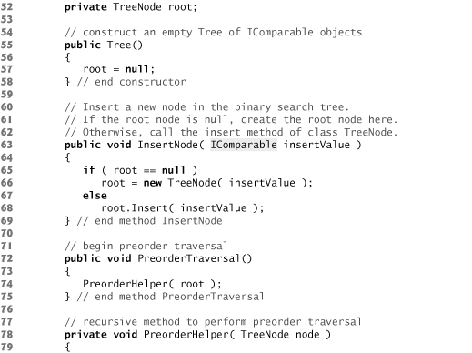
Methods InorderTraversal, PreorderTraversal and PostorderTraversal call helper methods InorderHelper (lines 100–113), PreorderHelper (lines 78–91) and PostorderHelper (lines 122–135), respectively, to traverse the tree and display the node values. The purpose of the helper methods in class Tree is to allow the programmer to start a traversal without needing to obtain a reference to the root node first, then call the recursive method with that reference. Methods InorderTraversal, PreorderTraversal and PostorderTraversal simply take private variable root and pass it to the appropriate helper method to initiate a traversal of the tree. For the following discussion, we use the binary search tree shown in Fig. 21.22.

Fig. 21.22. Binary search tree.

Inorder Traversal Algorithm

Method InorderHelper (lines 100–113) defines the steps for an inorder traversal. Those steps are as follows:

1. If the argument is null, do not process the tree.
2. Traverse the left subtree with a call to InorderHelper (line 105).
3. Process the value in the node (line 108).
4. Traverse the right subtree with a call to InorderHelper (line 111).

The inorder traversal does not process the value in a node until the values in that node’s left subtree are processed. The inorder traversal of the tree in Fig. 21.22 is

6 13 17 27 33 42 48

The inorder traversal of a binary search tree displays the node values in ascending order. The process of creating a binary search tree actually sorts the data (when coupled with an inorder traversal)—thus, this process is called the binary-tree sort.

Preorder Traversal Algorithm

Method PreorderHelper (lines 78–91) defines the steps for a preorder traversal. Those steps are as follows:

1. If the argument is null, do not process the tree.
2. Process the value in the node (line 83).
3. Traverse the left subtree with a call to PreorderHelper (line 86).
4. Traverse the right subtree with a call to PreorderHelper (line 89).

The preorder traversal processes the value in each node as the node is visited. After processing the value in a given node, the preorder traversal processes the values in the left subtree, then the values in the right subtree. The preorder traversal of the tree in Fig. 21.22 is

27 13 6 17 42 33 48

Postorder Traversal Algorithm

Method PostorderHelper (lines 122–135) defines the steps for a postorder traversal. Those steps are as follows:

1. If the argument is null, do not process the tree.
2. Traverse the left subtree with a call to PostorderHelper (line 127).
3. Traverse the right subtree with a call to PostorderHelper (line 130).
4. Process the value in the node (line 133).

The postorder traversal processes the value in each node after the values of all that node’s children are processed. The postorder traversal of the tree in Fig. 21.22 is

6 17 13 33 48 42 27

Duplicate Elimination

A binary search tree facilitates duplicate elimination. While building a tree, the insertion operation recognizes attempts to insert a duplicate value, because a duplicate follows the same “go left” or “go right” decisions on each comparison as the original value did. Thus, the insertion operation eventually compares the duplicate with a node containing the same value. At this point, the insertion operation might simply discard the duplicate value.

Searching a binary tree for a value that matches a key value is fast, especially for tightly packed binary trees. In a tightly packed binary tree, each level contains about twice as many elements as the previous level. Figure 21.22 is a tightly packed binary tree. A binary search tree with n elements has a minimum of log₂n levels. Thus, at most log₂n comparisons are required either to find a match or to determine that no match exists. Searching a (tightly packed) 1000-element binary search tree requires at most 10 comparisons, because ²¹⁰ > 1000. Searching a (tightly packed) 1,000,000-element binary search tree requires at most 20 comparisons, because 2²⁰ > 1,000,000.

Level-Order Traversal

A level-order traversal of a binary tree visits the nodes of the tree row by row, starting at the root-node level. On each level of the tree, a level-order traversal visits the nodes from left to right.

21.7.2 Binary Search Tree of IComparable Objects

The binary-tree example in Section 21.7.1 works nicely when all the data is of type int. Suppose that you want to manipulate a binary tree of doubles. You could rewrite the TreeNode and Tree classes with different names and customize the classes to manipulate doubles. Similarly, for each data type you could create customized versions of classes TreeNode and Tree. This proliferates code, and can become difficult to manage and maintain.

Ideally, we’d like to define the binary tree’s functionality once and reuse it for many types. Languages like C# provide polymorphic capabilities that enable all objects to be manipulated in a uniform manner. Using such capabilities enables us to design a more flexible data structure. C# provides these capabilities with generics (Chapter 22).

In our next example, we take advantage of C#’s polymorphic capabilities by implementing TreeNode and Tree classes that manipulate objects of any type that implements interface IComparable (namespace System). It is imperative that we be able to compare objects stored in a binary search, so we can determine the path to the insertion point of a new node. Classes that implement IComparable define method CompareTo, which compares the object that invokes the method with the object that the method receives as an argument. The method returns an int value less than zero if the calling object is less than the argument object, zero if the objects are equal and a positive value if the calling object is greater than the argument object. Also, both the calling and argument objects must be of the same data type; otherwise, the method throws an ArgumentException.

Figures 21.23–21.24 enhance the program of Section 21.7.1 to manipulate IComparable objects. One restriction on the new versions of classes TreeNode and Tree is that each Tree object can contain objects of only one type (e.g., all strings or all doubles). If a program attempts to insert multiple types in the same Tree object, ArgumentExceptions will occur. We modified only five lines of code in class TreeNode (lines 14, 20, 28, 30 and 38) and one line of code in class Tree (line 63) to enable processing of IComparable objects. Except for lines 30 and 38, all other changes simply replaced int with IComparable. Lines 30 and 38 previously used the < and > operators to compare the value being inserted with the value in a given node. These lines now compare IComparable objects via the interface’s CompareTo method, then test the method’s return value to determine whether it is less than zero (the calling object is less than the argument object) or greater than zero (the calling object is greater than the argument object), respectively. [Note: If this class were written using generics, the type of data, int or IComparable, could be replaced at compile time by any other type that implements the necessary operators and methods.]

Fig. 21.23. Declaration of class TreeNode.

Class TreeTest (Fig. 21.24) creates three Tree objects to store int, double and string values, all of which the .NET Framework defines as IComparable types. The program populates the trees with the values in arrays intArray (line 12), doubleArray (line 13) and stringArray (lines 14–15), respectively.

Fig. 21.24. Testing class Tree with IComparable objects.

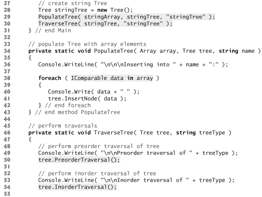
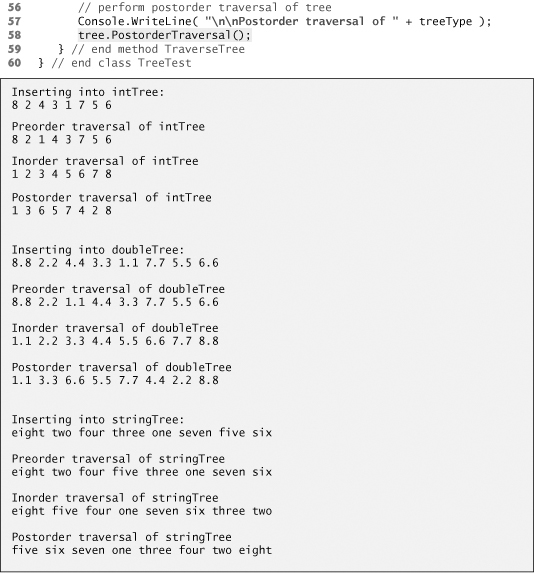
Method PopulateTree (lines 34–43) receives as arguments an Array containing the initializer values for the Tree, a Tree in which the array elements will be placed and a string representing the Tree name, then inserts each Array element into the Tree. Method TraverseTree (lines 46–59) receives as arguments a Tree and a string representing the Tree name, then outputs the preorder, inorder and postorder traversals of the Tree. The inorder traversal of each Tree outputs the data in sorted order regardless of the data type stored in the Tree. Our polymorphic implementation of class Tree invokes the appropriate data type’s CompareTo method to determine the path to each value’s insertion point by using the standard binary-search-tree insertion rules. Also, notice that the Tree of strings appears in alphabetical order.

21.8 Wrap-Up

In this chapter, you learned that simple types are value-type structs but can still be used anywhere objects are expected in a program due to boxing and unboxing conversions. You learned that linked lists are collections of data items that are “linked together in a chain.” You also learned that a program can perform insertions and deletions anywhere in a linked list (though our implementation performed insertions and deletions only at the ends of the list). We demonstrated that the stack and queue data structures are constrained versions of lists. For stacks, you saw that insertions and deletions are made only at the top—so stacks are known as last-in, first out (LIFO) data structures. For queues, which represent waiting lines, you saw that insertions are made at the tail and deletions are made from the head—so queues are known as first-in, first out (FIFO) data structures. We also presented the binary tree data structure. You saw a binary search tree that facilitated high-speed searching and sorting of data and efficient duplicate elimination. In the next chapter, we introduce generics, which allow you to declare a family of classes and methods that implement the same functionality on any type.