
6.2. Gaseous Fuel Jets
Diffusion flames have far greater practical application than premixed flames. Gaseous diffusion flames, unlike premixed flames, have no fundamental characteristic property, such as flame velocity, which can be measured readily; even initial mixture strength (the overall oxidizer-to-fuel ratio) has no practical meaning. Indeed, a mixture strength does not exist for a gaseous fuel jet issuing into a quiescent atmosphere. Certainly no mixture strength exists for a single small fuel droplet burning in the infinite reservoir of a quiescent atmosphere.

6.2.1. Appearance
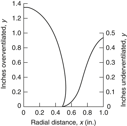
Only the shape of the burning laminar fuel jet depends on the mixture strength. If in a concentric configuration the volumetric flow rate of air flowing in the outer annulus is in excess of the stoichiometric amount required for the volumetric flow rate of the inner fuel jet, the flame that develops takes a closed, elongated form. A similar flame forms when a fuel jet issues into the quiescent atmosphere. Such flames are referred to as being overventilated. If in the concentric configuration the air supply in the outer annulus is reduced below an initial mixture strength corresponding to the stoichiometric required amount, a fan-shaped, underventilated flame is produced. The general shapes of the underventilated and overventilated flame are shown in Figure 6.2 and are generally referred to as co-flow configurations. As will be shown later in this chapter, the actual heights vary with the flow conditions.
The axial symmetry of the concentric configuration shown in Figure 6.2 is not conducive to experimental analyses, particularly when some optical diagnostic tools or thermocouples are used. There are parametric variations in the r and y coordinates shown in Figure 6.2. To facilitate experimental measurements on diffusion flames, the so-called Wolfhard–Parker two-dimensional gaseous fuel jet burner is used. Such a configuration is shown in Figure 6.3, taken from Smyth et al. [2]; the screens shown in the figure are used to stabilize the flame. As can be seen in Figure 6.3, ideally there are no parametric variations along the length of the slot.


Other types of gaseous diffusion flames are those in which the flow of the fuel and oxidizer oppose each other; these are referred to as counter-flow diffusion flames. The types most frequently used are shown in Figure 6.4. Although these configurations are somewhat more complex to establish experimentally, they have definite advantages. The opposed jet configuration, in which the reactant streams are injected as shown in Figure 6.4 as Types I and II, has two major advantages compared to co-flow fuel jet or Wolfhard–Parker burners. First, there is little possibility of oxidizer diffusion into the fuel side through the quench zone at the jet tube lip. Second, the flow configuration is more amenable to mathematical analysis.

Although the aerodynamic configuration designated as Types III and IV produce the stagnation point counter-flow diffusion flames shown, it is somewhat more experimentally challenging. More interestingly, the stability of the process is more sensitive to the flow conditions. Generally the mass flow rate through the porous media is very much smaller than the free stream flow. Usually the fuel bleeds through the porous medium, and the oxidizer is the free stream component. Of course, the reverse could be employed in such an arrangement. However, it is difficult to distinguish the separation of the flame and flow stagnation planes of the opposing flowing streams. Both, of course, are usually close to the porous body. This condition is alleviated by the approach shown by Types I and II in Figure 6.4.
As one will note from these figures, for a hydrocarbon fuel opposing an oxidizer stream (generally air), the soot formation region that is created and the flame front can lie on either side of the flow stagnation plane. In essence, although most of the fuel is diverted by the stagnation plane, some molecules diffuse through the stagnation plane to create the flame on the oxidizer side. With the diffusion flame located on the oxidizer side, the gas flow velocity (and thermophoresis) directs the soot particles, which are always formed on the fuel side of the flame, away from the high-temperature region of the diffusion flame. Because soot particles approximately follow the gas-phase streamlines, they are not oxidized. For the contra condition, when the diffusion flame and soot region reside on the fuel side of the stagnation plane, the soot particles are carried toward the high-temperature diffusion flame by the gas and thermophoretic velocities and have the potential to oxidize after passage through the flame. In the overventilated co-flow diffusion flame of Figure 6.2, the soot particles also move toward the flame and thus have similar path and temperature histories as when the counter-flow diffusion flame is located on the fuel side of the stagnation plane. In fact, a liquid hydrocarbon droplet burning in a quiescent environment mimics this configuration. With the diffusion flame on the oxidizer side, the soot formation and particle growth are very much different from any real combustion application.
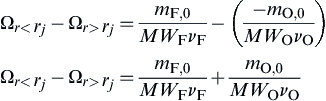
As Kang et al. [3] have reported, counter-flow diffusion flames are located on the oxidizer side when hydrocarbons are the fuel. Appropriate dilution with inert gases of both the fuel and oxidizer streams, frequently used in the co-flow situation, can position the flame on the fuel side. It has been shown [4] that the criterion for the flame to be located on the fuel side is.

where mO,0 is the free stream mass fraction of the oxidizer, mF,0 is the free stream mass fraction of the fuel, i is the mass stoichiometric coefficient, and Le is the appropriate Lewis number (see Chapter 4, Section 4.3.2). The Le for oxygen is 1 and for hydrocarbons it is normally greater than 1.
The profiles designating the flame height yF in Figure 6.2 correspond to the stoichiometric adiabatic flame temperature as developed in Section 6.2.4. Indeed, the curved shape designates the stoichiometric adiabatic flame temperature isotherm. However, when one observes an overventilated co-flow flame in which a hydrocarbon constitutes the fuel jet, one observes that the color of the flame is distinctly different from that of its premixed counterpart. Whereas a premixed hydrocarbon-air flame is violet or blue green, the corresponding diffusion flame varies from bright yellow or orange. The color of the hydrocarbon diffusion flame arises from the formation of soot in the fuel of the jet flame. The soot particles then flow through the reaction zone and reach the flame temperature. Some continue to burn through and after the flame zone and radiate. Due to the temperature that exists and the sensitivity of the eye to various wavelengths in the visible region of the electromagnetic spectrum, hydrocarbon-air diffusion flames, particularly those of co-flow structure, appear to be yellow or orange.
As will be discussed extensively in Chapter 8, Section 8.5, the hydrocarbon fuel pyrolyzes within the jet and a small fraction of the fuel forms soot particles that grow in size and mass before entering the flame. The soot continues to burn as it passes through the stoichiometric isotherm position that designates the fuel–air reaction zone and the true flame height. These high-temperature particles continue to burn and stay luminous until they are consumed in the surrounding flowing air. The end of the luminous yellow or orange image designates the soot burnout distance and not what one would call the stoichiometric flame temperature isotherm. For hydrocarbon diffusion flames, the visual distance from the jet port to the end of the “orange or yellow” flame is determined by the mixing of the burned gas containing soot with the overventilated air flow. Thus the faster the velocity of the co-flow air stream, the shorter the distance of the particle burnout. Simply, the particle burnout is not controlled by the reaction time of oxygen and soot, but by the mixing time of the hot exhaust gases and the overventilated gas stream. Thus, hydrocarbon fuel jets burning in quiescent atmospheres appear longer than in an overventilated condition. Non-sooting diffusion flames, such as those found with H2, CO, and methanol, are mildly visible and look very much like their premixed counterparts. Their true flame height can be estimated visually.
6.2.2. Structure
Unlike premixed flames, which have a very narrow reaction zone, diffusion flames have a wider region over which the composition changes and chemical reaction can take place. Obviously, these changes are due principally to some interdiffusion of reactants and products. Hottel and Hawthorne [5] were the first to make detailed measurements of species distributions in a concentric laminar H2-air diffusion flame. Figure 6.5 shows the type of results they obtained for a radial distribution at a height corresponding to a cross-section of the overventilated flame depicted in Figure 6.2. Smyth et al. [2] made very detailed and accurate measurements of temperature and species variation across a Wolfhard–Parker burner in which methane was the fuel. Their results are shown in Figures 6.6 and 6.7.
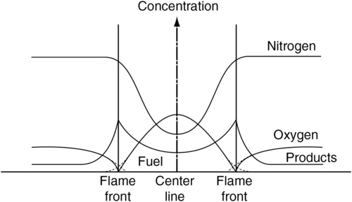
The flame front can be assumed to exist at the point of maximum temperature, and indeed this point corresponds to that at which the maximum concentrations of major products (CO2 and H2O) exist. The same type of profiles would exist for a simple fuel jet issuing into quiescent air. The maxima arise due to diffusion of reactants in a direction normal to the flowing streams. It is most important to realize that, for the concentric configuration, molecular diffusion establishes a bulk velocity component in the normal direction. In the steady state, the flame front produces a flow outward, molecular diffusion establishes a bulk velocity component in the normal direction, and oxygen plus a little nitrogen flows inward toward the centerline. In the steady state, the total volumetric rate of products is usually greater than the sum of the other two. Thus, the bulk velocity that one would observe moves from the flame front outward. The oxygen between the outside stream and the flame front then flows in the direction opposite to the bulk flow. Between the centerline and the flame front, the bulk velocity must, of course, flow from the centerline outward. There is no sink at the centerline. In the steady state, the concentration of the products reaches a definite value at the centerline. This value is established by the diffusion rate of products inward and the amount transported outward by the bulk velocity.

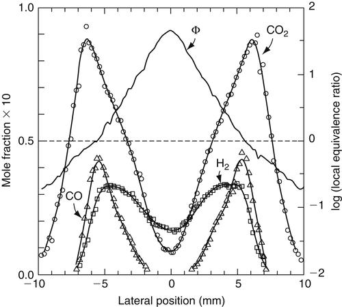
Since total disappearance of reactants at the flame front would indicate infinitely fast reaction rates, a more likely graphical representation of the radial distribution of reactants should be that given by the dashed lines in Figure 6.5. To stress this point, the dashed lines are drawn to grossly exaggerate the thickness of the flame front. Even with finite reaction rates, the flame front is quite thin. The experimental results shown in Figures 6.6 and 6.7 indicate that in diffusion flames the fuel and oxidizer diffuse toward each other at rates that are in stoichiometric proportions. Since the flame front is a sink for both the fuel and oxidizer, intuitively one would expect this most important observation. Independent of the overall mixture strength, since fuel and oxidizer diffuse together in stoichiometric proportions, the flame temperature closely approaches the adiabatic stoichiometric flame temperature. It is probably somewhat lower due to finite reaction rates, that is, approximately 90% of the adiabatic stoichiometric value [6] whether it is a hydrocarbon fuel or not. This observation establishes an interesting aspect of practical diffusion flames in that for an adiabatic situation two fundamental temperatures exist for a fuel: one that corresponds to its stoichiometric value and occurs at the flame front, and one that occurs after the products mix with the excess air to give an adiabatic temperature that corresponds to the initial mixture strength.
6.2.3. Theoretical Considerations
The theory of premixed flames essentially consists of an analysis of factors such as mass diffusion, heat diffusion, and the reaction mechanisms as they affect the rate of homogeneous reactions taking place. Inasmuch as the primary mixing processes of fuel and oxidizer appear to dominate the burning processes in diffusion flames, the theories emphasize the rates of mixing (diffusion) in deriving the characteristics of such flames.
It can be verified easily by experiments that in an ethylene-oxygen premixed flame, the average rate of consumption of reactants is about 4 mol/cm3s, whereas for the diffusion flame (by measurement of flow, flame height, and thickness of reaction zone—a crude, but approximately correct approach), the average rate of consumption is only 6 × 10⁻⁵ mol/cm3s. Thus, the consumption and heat release rates of premixed flames are much larger than those of pure mixing-controlled diffusion flames.
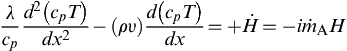
The theoretical solution to the diffusion flame problem is best approached in the overall sense of a steady flowing gaseous system in which both the diffusion and chemical processes play a role. Even in the burning of liquid droplets, a fuel flow due to evaporation exists. This approach is much the same as that presented in Chapter 4, Section 4.3.2, except that the fuel and oxidizer are diffusing in opposite directions and in stoichiometric proportions relative to each other. If one selects a differential element along the x-direction of diffusion, the conservation balances for heat and mass may be obtained for the fluxes, as shown in Figure 6.8.
In Figure 6.8, j is the mass flux as given by a representation of Fick's law when there is bulk movement. From Fick's law:
![]()

As will be shown in Section 6.3.2, the following form of j is exact (however, the same form can be derived if it is assumed that the total density does not vary with the distance x, as of course it actually does):
![]()
where mA is the mass fraction of species A. In Figure 6.8, q is the heat flux given by Fourier's law of heat conduction;  is the rate of decrease of mass of species A in the volumetric element (Δx·1)(g/cm3s), and
  is the rate of chemical energy release in the volumetric element (Δx·1)(cal/cm3s).
With the preceding definitions, for the one-dimensional problem defined in Figure 6.8, the expression for conservation of a species A (say the oxidizer) is:
![]() (6.1)
(6.1)
where ρ is the total mass density, ρA is the partial density of species A, and υ is the bulk velocity in direction x. Solving this time-dependent diffusion flame problem is outside the scope of this text. Indeed, most practical combustion problems have a steady fuel mass input. Thus, for the steady problem, which implies steady mass consumption and flow rates, one may not only take ∂ρA/∂t as zero but also use the following substitution:
![]() (6.2)
(6.2)
The term (ρυ) is a constant in the problem since there are no sources or sinks. With the further assumption from simple kinetic theory that Dρ is independent of temperature, and hence of x, Eqn (6.1) becomes:
![]() (6.3)
(6.3)
Obviously, the same type of expression must hold for the other diffusing species B (say the fuel), even if its gradient is opposite to that of A, so that:
![]() (6.4)
(6.4)
where  is the rate of decrease of species B in the volumetric element (Δx·1) and i is the mass stoichiometric coefficient:
![]()
 (6.5)
(6.5)
where is the rate of chemical energy release per unit volume, and H is the heat release per unit mass of fuel consumed (in joules per gram), that is:
![]() (6.6)
(6.6)
since must be negative for heat release (exothermic reaction) to take place.
Although the form of Eqns (6.3)–(6.5) is the same as that obtained in dealing with premixed flames, an important difference lies in the boundary conditions that exist. Furthermore, in comparing Eqns (6.3) and (6.4) with Eqns (4.31) and (4.32), one must realize that in Chapter 4, the mass change symbol  was always defined as a negative quantity.
Multiplying Eqn (6.3) by iH, and then combining it with Eqn (6.5) for the condition Le = 1 or ρD = (λ/cp), one obtains:
![]() (6.7)
(6.7)
This procedure is sometimes referred to as the Schvab–Zeldovich transformation. Mathematically, what has been accomplished is that the nonhomogeneous terms ( and ) have been eliminated and a homogeneous differential equation (Eqn (6.7)) has been obtained.
The equations could have been developed for a generalized coordinate system. In a generalized coordinate system, they would have the form:
![]() (6.8)
(6.8)
![]() (6.9)
(6.9)
These equations could be generalized even further (see Ref. [7]) by simply writing  instead of , where
  is the heat of formation per unit mass at the base temperature of each species j. However, for notation simplicity—and because energy release is of most importance for most combustion and propulsion systems—an overall rate expression for a reaction of the type which follows will suffice:
![]() (6.10)
(6.10)
where F is the fuel, O the oxidizer, P the product, and ϕ the molar stoichiometric index. Then Eqns (6.8) and (6.9) may be written as:
![]() (6.11)
(6.11)
![]() (6.12)
(6.12)
where MW is the molecular weight,  for the oxidizer, and νj = 1 for the fuel. Both equations have the form:
![]() (6.13)
(6.13)
where αT = cpT/(H MWjνj) and αj = mj/(MWjνj). They may be expressed as:
![]() (6.14)
(6.14)
where the linear operation L(α) is defined as:
![]() (6.15)
(6.15)
The nonlinear term may be eliminated from all but one of the relationships  For example:
![]() (6.16)
(6.16)
can be solved for α1, then the other flow variables can be determined from the linear equations for a simple coupling function Ω so that:
![]() (6.17)
(6.17)
where Ω = (αj − αl) ≡ Ωj (j ≠ 1). Obviously if 1 = fuel and there is a fuel–oxidizer system only, j = 1 gives Ω = 0 and shows the necessary redundancy.
6.2.4. The Burke–Schumann Development
With the development in the previous section, it is now possible to approach the classical problem of determining the shape and height of a burning gaseous fuel jet in a coaxial stream as first described by Burke and Schumann and presented in detail in Lewis and von Elbe [8].
This description is given by the following particular assumptions:
1. At the port position, the velocities of the air and fuel are considered constant, equal, and uniform across their respective tubes. Experimentally, this condition can be obtained by varying the radii of the tubes (see Figure 6.2). The molar fuel rate is then given by the radii ratio:

2. The velocity of the fuel and air up the tube in the region of the flame is the same as the velocity at the port.
3. The coefficient of interdiffusion of the two gas streams is constant.
Burke and Schumann [9] suggested that the effects of assumptions 2 and 3 compensate for each other, thereby minimizing errors. Although D increases as T1.67 and velocity increases as T, this disparity should not be the main objection. The main objection should be the variation of D with T in the horizontal direction due to heat conduction from the flame.
4. Interdiffusion is entirely radial.
5. Mixing is by diffusion only, that is, there are no radial velocity components.
6. Of course, the general stoichiometric relation prevails.
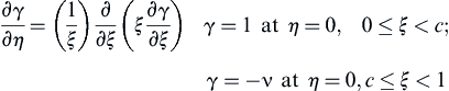
With these assumptions, one may readily solve the coaxial jet problem. The only differential equation that one is obliged to consider is:
![]()
where αF = +mF/MWFνF and αO = +mO/MWOνO. In cylindrical coordinates, the generation equation becomes:
![]() (6.18)
(6.18)
The cylindrical coordinate terms in ∂/∂θ are set equal to zero because of the symmetry. The boundary conditions become:

and  at r = rs, y > 0. In order to achieve some physical insight to the coupling function Ω, one should consider it as a concentration or, more exactly, a mole fraction. At y = 0 the radial concentration difference is:
This difference in Ω reveals that the oxygen acts as it were a negative fuel concentration in a given stoichiometric proportion, or vice versa. This result is, of course, a consequence of the choice of the coupling function and the assumption the fuel and oxidizer approach each other in stoichiometric proportion.
It is convenient to introduce dimensionless coordinates:
![]()
and to define parameters c ≡ rj/rs, an initial molar mixture strength ν:
![]()
![]()
Equation (6.18) and the boundary conditions then become:
and:
![]() (6.19)
(6.19)
Equation (6.19), with these new boundary conditions, has the known solution:
 (6.20)
where J0 and J1 are Bessel functions of the first kind (of order 0 and 1, respectively), and the ϕn represent successive roots of the equation J1 (ϕ) = 0 (with the ordering convention ϕn > ϕn−1, ϕ0 = 0). This equation gives the solution for Ω in the present problem.
The flame shape is defined at the point where the fuel and oxidizer disappear, that is, the point that specifies the place where Ω = 0. Hence, setting γ = 0 provides a relation between ξ and η that defines the locus of the flame surface.
The equation for the flame height is obtained by solving Eqn (6.20) for η after setting ξ = 0 for the overventilated flame and ξ = 1 for the underventilated flame (also γ = 0).
The resulting equation is still very complex. Since flame heights are large enough to cause the factor  to decrease rapidly as n increases at these values of η, it usually suffices to retain only the first few terms of the sum in the basic equation for this calculation. Neglecting all terms except n = 1, one obtains the rough approximation:
 (6.21)
for the dimensionless height of the overventilated flame. The first zero of J1 (ϕ) is ϕ1 = 3.83.
The flame shapes and heights predicted by such expressions (see Figure 6.9) are shown by Lewis and von Elbe [8] to be in good agreement with experimental results—surprisingly so, considering the basic drastic assumptions.
Indeed, it should be noted that Eqn (6.21) specifies that the dimensionless flame height can be written as:
![]() (6.22)
(6.22)
Thus since c = (rj/rs), the flame height can also be represented by:
![]() (6.23)
(6.23)
where υ is the average fuel velocity, Q is the volumetric flow rate of the fuel, and f′ = (f/c2). Thus, one observes that the flame height of a circular fuel jet is directly proportional to the volumetric flow rate of the fuel.
In a pioneering paper [10], Roper vastly improved on the Burke–Schumann approach to determine flame heights not only for circular ports but also for square ports and slot burners. Roper's work is significant because he used the fact that the Burke–Schumann approach neglects buoyancy and assumes the mass velocity should everywhere be constant and parallel to the flame axis to satisfy continuity [7], and then pointed out that resulting errors cancel for the flame height of a circular port burner but not for the other geometries [10,11]. In the Burke–Schumann analysis, the major assumption is that the velocities are everywhere constant and parallel to the flame axis. Considering the case in which buoyancy forces increase the mass velocity after the fuel leaves the burner port, Roper showed that continuity dictates decreasing streamline spacing as the mass velocity increases. Consequently, all volume elements move closer to the flame axis, the widths of the concentration profiles are reduced, and the diffusion rates are increased.
Roper [10] also showed that the velocity of the fuel gases is increased due to heating, and that the gases leaving the burner port at temperature T0 rapidly attain a constant value Tf in the flame regions controlling diffusion; thus the diffusivity in the same region is:
![]()
where D0 is the ambient or initial value of the diffusivity. Then, considering the effect of temperature on the velocity, Roper developed the following relationship for the flame height:
 (6.24)
where S is the stoichiometric volume rate of air to volume rate of fuel. Although Roper's analysis does not permit calculation of the flame shape, it does produce for the flame height a much simpler expression than Eqn (6.21).
If due to buoyancy the fuel gases attain a velocity υb in the flame zone after leaving the port exit, continuity requires that the effective radial diffusion distance be some value rb. Obviously, continuity requires that ρ be the same for both cases, so that:
![]()
Thus, one observes that regardless of whether the fuel jet is momentum- or buoyancy-controlled, the flame height yF is directly proportional to the volumetric flow leaving the port exit.
Given the condition that buoyancy can play a significant role, the fuel gases start with an axial velocity and continue with a mean upward acceleration g due to buoyancy. The velocity of the fuel gases υ is then given by:
![]() (6.25)
(6.25)
where υ is the actual velocity, υ0 is the momentum-driven velocity at the port, and υb is the velocity due to buoyancy. However, the buoyancy term can be closely approximated by:
![]() (6.26)
(6.26)
where g is the acceleration due to buoyancy. If one substitutes Eqn (6.26) into Eqn (6.25) and expands the result in terms of a binomial expression, one obtains:
 (6.27)
where the term in parentheses is the inverse of the modified Froude number:
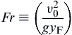 (6.28)
Thus, Eqn (6.27) can be written as:
![]() (6.29)
(6.29)
For large Froude numbers, the diffusion flame height is momentum-controlled and υ = υ0. However, most laminar burning fuel jets will have very small Froude numbers and υ = υb; that is, most laminar fuel jets are buoyancy-controlled.
Although the flame height is proportional to the fuel volumetric flow rate whether the flame is momentum- or buoyancy-controlled, the time to the flame tip does depend on what the controlling force is. The characteristic time for diffusion (tD) must be equal to the time (ts) for a fluid element to travel from the port to the flame tip; that is, if the flame is momentum-controlled:
 (6.30)
It follows from Eqn (6.30), of course, that:
![]() (6.31)
(6.31)
Equation (6.31) shows the same dependence on Q as that developed from the Burke–Schumann approach (Eqns (6.21)–(6.23)). For a momentum-controlled fuel jet flame, the diffusion distance is rj, the jet port radius; and from Eqn (6.30) it is obvious that the time to the flame tip is independent of the fuel volumetric flow rate. For a buoyancy-controlled flame, ts remains proportional to (yF/υ); however, since υ = (2gyF)1/2:
![]() (6.32)
(6.32)
Thus, the stay time of a fuel element in a buoyancy-controlled laminar diffusion flame is proportional to the square root of the fuel volumetric flow rate. This conclusion is significant with respect to the soot smoke height tests to be discussed in Chapter 8.
For low Froude number, a fuel leaving a circular jet port immediately becomes affected by a buoyancy condition, and the flame shape is determined by this condition and the consumption of the fuel. In essence, following Eqn (6.26) the velocity within the exit fuel jet becomes proportional to its height above the port exit as the flow becomes buoyantly controlled. For example, the velocity along the axis would vary according to the proportionality υ ∼ y−1/2. Thus, the velocity increases as it approaches the flame tip. Conservation of mass requires  = ρυA, where is the mass flow rate and ρ the density of the flowing gaseous fuel (or the fuel plus additives). Thus the flame shape contracts not only due to the consumption of the fuel but also as the buoyant velocity increases and a conical flame shape develops just above the port exit. For a constant mass flow buoyant system υ ∼ yF1/2 ∼ QF1/2. Thus υ ∼ P−1/2, and since the mass flow must be constant rather than affected by pressure change, = ρυA ∼ PP−1/2P−1/2 = constant. This proportionality states that, as the pressure of an experiment is raised, the planar cross-sectional area across any part of a diffusion flame must contract and take a narrower conical shape. This pressure effect has been clearly shown experimentally by Flowers and Bowman [12].
The preceding analyses hold only for circular fuel jets. Roper [10] has shown, and the experimental evidence verifies [11], that the flame height for a slot burner is not the same for momentum- and buoyancy-controlled jets. Consider a slot burner of the Wolfhard–Parker type in which the slot width is x and the length is L. As discussed earlier for a buoyancy-controlled situation, the diffusive distance would not be x, but some smaller width, say xb. Following the terminology of Eqn (6.25), for a momentum-controlled slot burner:
![]() (6.33)
(6.33)
and:
![]() (6.34)
(6.34)
For a buoyancy-controlled slot burner:
 (6.35)
 (6.36)
Recalling that xb must be a function of the buoyancy, one has:

Thus Eqn (6.36) becomes:
 (6.37)
Comparing Eqns (6.34) and (6.37), one notes that under momentum-controlled conditions for a given Q, the flame height is directly proportional to the slot width, while that under buoyancy-controlled conditions for a given Q, the flame height is independent of the slot width. Roper et al. [11] have verified these conclusions experimentally.
6.2.5. Conserved Scalars and Mixture Fraction
The simple coupling function Ω introduced in the last two sections is an example of a conserved scalar, which is a property that is conserved throughout the flow field being neither created nor destroyed by chemical reaction. As shown in the previous section, the classical approach to solving diffusion flame problems is to describe the mixing by obtaining a solution for a conserved scalar. The assumption of fast chemistry implies that the species concentrations and temperature are functions only of the conserved scalar. There are many scalar variables that are conserved. When the chemistry is simplified to a one-step reaction, simple conserved scalars may be used, as was done in the previous sections. If the one-step reaction is written in terms of mass quantities instead of molar coefficients as:
![]()
where MWFνF = 1 and MWOνO = r, and recognizing that:
![]()
the following conserved scalars are attained among the fuel, oxidizer, and product, which are examples of coupling functions [13]:

As shown previously, coupling functions can also be formed using the sensible enthalpy. Simple conserved scalars are all linearly related so that the solution for one yields all of the others.
For a one-step reaction, the mixture fraction (Z), also a conserved scalar, can be defined in terms of the fuel oxidizer coupling function having a value of 1 in the fuel stream and a value of 0 in the oxidizer stream:
![]()
where ΩF,0 and ΩO,0 are the values of Ω (= αF − αO) evaluated in the fuel and oxidizer streams (e.g., at the entrance boundary or infinity), respectively.
In systems that are more complex, one particular conserved scalar may be favored over another, for example, in systems with non-equal diffusivity, systems with more than one feed for the fuel or oxidizer, or systems with complex chemistry. With multistep reaction mechanisms, conserved scalars based on the species elements are generally used. The local mass fraction of element j may be defined as:
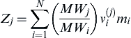
where MWj is the atomic weight of element j, MWi the molecular weight of species i, and  the number of atoms of type j in species i. With the mixture fraction defined as the mass of material having its origin in the fuel stream relative to the mass of the mixture, the mixture fraction may be defined as:
![]()
where the element j does not have the same value of Zj in each stream. Again, Z is unity in the fuel stream and zero in the oxidizer stream. Using the mixture fraction coordinate versus x or r, profiles of temperature and species concentration are much less strongly coupled on the flow configuration [7,14]. The mixture fraction is an important descriptor of diffusion flames and has been shown useful in describing the structure of turbulent flames [7,14].
6.2.6. Turbulent Fuel Jets
Section 6.2.4 considered the burning of a laminar fuel jet, and the essential result with respect to flame height was that:
 (6.38)
where yF,L specifies the flame height. When the fuel jet velocity is increased to the extent that the flow becomes turbulent, the Froude number becomes large and the system becomes momentum-controlled—moreover, molecular diffusion considerations lose their validity under turbulent fuel jet conditions. One would intuitively expect a change in the character of the flame and its height. Turbulent flows are affected by the occurrence of flames, as discussed for premixed flame conditions, and they are affected by diffusion flames by many of the same mechanisms discussed for premixed flames. However, the diffusion flame in a turbulent mixing layer between the fuel and oxidizer streams steepens the maximum gradient of the mean velocity profile somewhat and generates vorticity of opposite signs on opposite sides of the high-temperature, low-density reaction region.
The decreased overall density of the mixing layer with combustion increases the dimensions of the large vortices and reduces the rate of entrainment of fluids into the mixing layer [14]. Thus it is appropriate to modify the simple phenomenological approach that led to Eqn (6.31) to account for turbulent diffusion by replacing the molecular diffusivity with a turbulent eddy diffusivity. Consequently, the turbulent form of Eqn (6.38) becomes:

where yF,T is the flame height of a turbulent fuel jet. But ε ∼ lU′, where l is the integral scale of turbulence, which is proportional to the tube diameter (or radius rj), and U′ is the intensity of turbulence, which is proportional to the mean flow velocity υ along the axis. Thus one may assume that:
![]() (6.39)
(6.39)
Combining Eqn (6.39) and the preceding equation, one obtains:
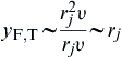 (6.40)
This expression reveals that the height of a turbulent diffusion flame is proportional to the port radius (or diameter) above, irrespective of the volumetric fuel flow rate or fuel velocity issuing from the burner! This important practical conclusion has been verified by many investigators.
The earliest verification of yF,T ∼ rj was by Hawthorne et al. [15], who reported their results as yF,T as a function of jet exit velocity from a fixed tube exit radius. Thus varying the exit velocity is the same as varying the Reynolds number. The results in Ref. [15] were represented by Linan and Williams [14] in the diagram duplicated here as Figure 6.10. This figure clearly shows that as the velocity increases in the laminar range, the height increases linearly, in accordance with Eqn (6.38). After transition to turbulence, the height becomes independent of the velocity, in agreement with Eqn (6.40). Observing Figure 6.10, one notes that the transition to turbulence begins near the top of the flame; then as the velocity increases, the turbulence rapidly recedes to the exit of the jet. At a high enough velocity, the flow in the fuel tube becomes turbulent, and turbulence is observed everywhere in the flame. Depending on the fuel mixture, liftoff usually occurs after the flame becomes fully turbulent. As the velocity increases further after liftoff, the liftoff height (the axial distance between the fuel jet exit and the point where combustion begins) increases approximately linearly with the jet velocity [14]. After the liftoff height increases to such an extent that it reaches a value comparable to the flame diameter, a further increase in the velocity causes blowoff [14].

..................Content has been hidden....................
You can't read the all page of ebook, please click here login for view all page.