
Chapter 42
Reliability
The reliability of electronic equipment can to some extent be quantified, and a separate discipline of reliability engineering has grown up to address it. This chapter will serve as an introduction to the subject for those circuit designers who are not fortunate enough to have a reliability engineering department at their disposal.
42.1 Definitions
Reliability, itself, has a strictly defined meaning. This can be stated as “the probability that a system will operate without failure for a specified period, subject to specified environmental conditions.” Thus, it can be quoted as a single number, such as 90%, but this is subject to three qualifications:
• Agreement as to what constitutes a “failure.” Many systems may “fail” without becoming totally useless in the process.
• A specified operating lifetime. No equipment will operate forever; reliability must refer to the reasonably foreseen operating life of the equipment, or to some other agreed period. The age of the equipment, which may well affect failure rate, is not a factor in the reliability specification.
• Agreement upon environmental conditions. Temperature, moisture, corrosive atmospheres, dust, vibration, shock, supply and electromagnetic disturbances all have an effect on equipment operation and reliability is meaningless if these are not quoted.
If you offer or purchase equipment whose reliability is quoted for one set of conditions and it is used under another set, you will not be able to extrapolate the reliability figure to the new conditions unless you know the behavior of those parameters which affect it.
42.1.2 Mean Time Between Failures
For most of the life of a piece of electronic equipment, its failure rate (denoted by λ) is constant. In the early stages of operation it could be high and decrease as weak components fail quickly and are replaced; late in its life components may begin to “wear out” or corrosion may take its toll, and the failure rate may start to rise again. The reciprocal of failure rate during the constant period is known as the mean time between failures (MTBF). This is generally quoted in hours, while failure rate is quoted in faults per hour. For instance, an MTBF of 10,000 hours is equivalent to a failure rate of 0.0001 faults per hour or 100 faults per 106 hours. MTBF has the advantage that it does not depend on the operating period, and is therefore more convenient to use than reliability.
42.1.3 Mean Time to Failure
MTBF measures equipment reliability on the assumption that it is repaired on each failure and put back into service. For components which are not repairable, their reliability is quoted as mean time to failure (MTTF). This can be calculated statistically by observing a sample from a batch of components and recording each one’s working life, a procedure known as life testing. The MTTF for this batch is then given by the mean of the lifetimes.
42.1.4 Availability
System users need to know for what proportion of time their system will be available to them. This figure is given by the ratio of “up-time,” during which the system is switched on and working, to total operating time. The difference between the two is the “down-time” during which the system is faulty and/or under repair. Thus:
![]()
Availability can also be related to the MTBF figure and the mean time to repair (MTTR) figure by:
![]()
The availability of a particular system can be monitored by logging its operating data, and this can be used to validate calculated MTBF and MTTR figures. It can also be interpreted as a probability that at any given instant the system will be found to be working.
42.2 The Cost of Reliability
Reliability does not come for free. Design and development costs escalate as more effort is put into assuring it, and component costs increase if high performance is required of them. For instance, it would be quite possible to improve the reliability of, say, an audio power amplifier by using massively over-rated output transistors, but these would add considerably to the selling cost of the amplifier. On the other hand, if the selling cost were reduced by specifying under-rated transistors, the users would find their total operating costs mounting since the output transistors would have to be replaced more frequently. Thus there is a general trend of decreasing operating or “lifecycle” costs and increasing unit costs, as the designed-in reliability of a given system increases. This leads to the notion of an “optimum” reliability figure in terms of cost for a system. Figure 42.1 illustrates this trend. The criterion of good design is then to approach this optimum as closely as possible.
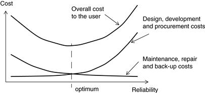
Figure 42.1 Reliability vs. cost
Of course, this argument only applies when the cost of unreliability is measured in strictly economic terms. Safety-critical systems, such as nuclear or chemical process plant controllers, railway signaling or flight-critical avionics, must instead meet a defined reliability standard and the design criterion then becomes one of assuring this level of reliability, with cost being a secondary factor.
42.3 Design for Reliability
The goal of any circuit designer is to reduce the failure rate of their design to the minimum achievable within cost constraints. The factors that help in meeting this goal are:
• use effective thermal management to minimize temperature rise;
• de-rate susceptible components as far as possible;
• specify high reliability or quality assured components;
• specify stress screening or burn-in tests;
• keep circuits simple, use the minimum number of components; and
42.3.1 Temperature
High temperature is the biggest enemy of all electronic components and measures to keep it down are vital. Temperature rise accelerates component breakdown because chemical reactions occurring within the component, which govern bond fractures, growth of contamination or other processes, have an increased rate of reaction at higher temperature. The rate of reaction is determined by the Arrhenius equation,
![]()
where,
λ gives a measure of failure rate
K is a constant depending on the component type
E is the reaction’s activation energy
Many reactions have activation energies around 0.5eV which results in an approximate doubling of λ with every 10°C rise in temperature, and this is a useful rule of thumb to apply for the decrease in reliability versus temperature of typical electronic equipment with many components. Some reactions have higher activation energy, which give a faster increase of λ with temperature.
42.3.2 De-Rating
There is a very significant improvement to be gained by operating a component well within its nominal rating. For most components this means either its voltage or power rating, or both.
Take capacitors as an example. Conventionally, you will determine the maximum DC bias voltage a capacitor will have to withstand under worst-case conditions and then select the next highest rating. Overspecifying the voltage rating may result in a larger and more costly component.
However, capacitor life tests show that as the maximum working voltage is approached, the failure rate increases as the fifth power of the voltage. Therefore, if you run the capacitor at half its rated voltage you will observe a failure rate 32 times lower than if it is run at full rated voltage. Given that a capacitor of double the required rating will not be as much as double the size, weight or cost, except at the extremes of range, the improvement in reliability is well worth having.
In many cases there is no difficulty in using a de-rated capacitor; small film capacitors, for instance, are rated at a minimum of 50 or 100V and are frequently used in 5V circuits. Electrolytics on the other hand are more likely to be run near their rating. These capacitors already have a much higher failure rate than other types because of their construction—the electrolyte has a tendency to “dry out,” especially at high temperatures—and so you will achieve significant improvement, albeit at higher cost, if you heavily de-rate them.
De-rating the power dissipation of resistors reduces their internal temperature and therefore their failure rate. In low voltage circuits there is no need to check power rating for any except low value parts; if for instance you use 0.4-watt metal film resistors in a circuit with a maximum supply of 10V, you can be sure that all resistors over 500ω will be de-rated by at least a factor of 2, which is normally enough.
Semiconductor devices are normally rated for power, current and voltage, and de-rating on all of these will improve failure rate. The most important are power dissipation, which is closely linked to junction temperature rise and cooling provision, and operating voltage, especially in the presence of possible transient overvoltages.
42.3.3 High Reliability Components
Component manufacturers’ reputations are seriously affected by the perceived reliability or otherwise of their product, so most will go to considerable effort not to ship defective parts. However, the cost of detecting and replacing a faulty part rises by an order of magnitude at each stage of the production process, starting at goods inward inspection, proceeding through board assembly, test and final assembly, and ending up with field repair. You may therefore decide (even in the absence of mandatory procurement requirements on the part of your customer) that it is worth spending extra to specify and purchase parts with a guaranteed reliability specification at the “front end” of production.
42.3.4 CECC
Initially it was military requirements, where reliability was more important than cost, that drove forward schemes for assessed quality components. More recently many commercial customers have also found it necessary to specify such components. The need for a common standard of assessed quality is met in Europe by the CECC† scheme. This has superseded the earlier national BS9000 series of standards. CECC documents refer to a “Harmonized system of quality assessment for electronic components.”
Generic specifications are found in the CECC series for all types of component which are covered by the scheme. These specify physical, mechanical and electrical properties, and lay down test requirements. Individual component specifications are not found under the scheme.
42.3.5 Stress Screening and Burn-in
These specifications all include some degree of stress screening. This phrase refers to testing the components under some type of stress, typically at elevated temperature, under vibration or humidity and with maximum rated voltage applied, for a given period. This practice is also called burning in. The principle is that weak components will fail early in their life and the failures can be accelerated by operating them under stress. These can then be weeded out before the parts are shipped from the manufacturer. A typical test might be 160 hours at 125°C. Another common test is a repeated temperature cycle between the extremes of the permitted temperature range, which exposes failures due to poor bonding or other mechanical faults.
Such stress screening can be applied to any component, not just semiconductors, and also to entire assemblies. If you are unsure of the probable quality of early production output of a new design, specifying stress screening on the first few batches is a good way to discover any recurrent production faults before they are passed out to the customer. It is expensive in time, equipment and inventory, and should not be used as a crutch to compensate for poor production practices. It should only be employed as standard if the customer is willing to pay for it.
42.3.6 Simplicity
The failure rate of an electronic assembly is roughly equal to the sum of the failure rates of all its components. This assumes that a failure in any one component causes the failure of the whole assembly. This is not necessarily a valid assumption, but to assume otherwise you would have to work out the assembly’s failure modes for each component failure and for combinations of failures, which is not practical unless your customer is prepared to pay for a great deal of development work.
If the assumption holds, then reducing the number of components will reduce the overall failure rate. This illustrates a very important principle in circuit design: the highest reliability comes from the simplest circuits. Apply Occam’s razor (“entities should not be multiplied beyond necessity”) and cut down the number of components to a minimum.
42.3.7 Redundancy
Redundancy is employed at the system level by connecting the outputs of two or more subsystems together such that if one fails, the others will continue to keep the system working. A typical example might be several power supplies, each connected to the same power distribution rail (via isolating diodes) and each capable of supplying the full load. If the reliability of the interconnection is neglected, the probability of all supplies failing simultaneously is the product of the probabilities of failure of each supply on its own, assuming that a common mode failure (such as the mains supply to all units going off) is ruled out.
The principle can also be applied at the component level. If the probability of a single component failing is too high then redundant components can be placed in parallel or series with it, depending on the required failure mode. This technique is mandatory in certain fields, such as intrinsically safe instrumentation. Figure 42.2 illustrates redundant zener diode clamping. The zeners prevent the voltage across their terminals from rising to an unsafe value in the event of a fault voltage being applied at the input to the barrier. One zener alone would not offer the required level of reliability, so two further ones are placed in parallel, so that even with an open-circuit failure of two out of the three, the clamping action is maintained. The interconnections between the zeners must be solid enough not to materially affect the reliability of the combination.

Figure 42.2 The intrinsically safe zener diode barrier
Some provision must normally be made for detecting and indicating a failed component or subsystem so that it can be repaired or replaced. Otherwise, once a redundant part has failed, the overall reliability of the system is severely reduced.
42.4 The Value of MTBF Figures
The mean time between failure figure as defined earlier can be calculated before the equipment is put into production by summing the failure rates of individual components to give an overall failure rate for the whole equipment. As discussed earlier, this assumes that a fault in any one component causes the failure of the whole assembly. This method presupposes adequate data on the expected failure rates of all components that will be used in the equipment.
Such sources of failure rate data for established component types are available. The most widely used is MIL-HDBK-217, now in its fifth revision, published by the US Department of Defense. This handbook lists failure rate models and tables for a wide variety of components, based on observed failure measurements. A failure rate for each component can be derived from its operating and environmental conditions, de-rating factor and method of construction or packaging. A further factor that is included for integrated circuits is their complexity and pinout. Another source of failure rate data, somewhat less comprehensive but widely used for telecommunications applications, is British Telecom’s handbook HRD4.
The disadvantage with using such data is that it cannot be up-to-date. Proper failure rate data takes years to accumulate, and so data extracted from these tables for modern components will not be accurate. This is especially true for integrated circuits. Generally, figures based on obsolete failure rate data will tend to be pessimistic, since the trend of component reliability is to improve.
Calculations of failure rates at component level are tedious, since operating conditions for each component, notably voltage and power dissipation, must be a part of the calculation in order to arrive at an accurate value. They do lend themselves to computer derivation, and software packages for reliability prediction are readily available. Since in many cases such operating conditions are highly variable, it is arguable that you will not obtain much more than an order-of-magnitude estimate of the true figure anyway.
A published MTBF figure does not tell you how long the unit will actually last, and it does not indicate how well the unit will perform in the field under different environmental and operating conditions. Such figures are mainly used by the marketing department to make the specification more attractive. But MTBF prediction is valuable for two purposes:
• For the designer, it gives an indication of where reliability improvements can most usefully be made. For instance, if as is often the case the electrolytic capacitors turn out to make the highest contribution to overall failure rate, you can easily evaluate the options available to you in terms of de-rating or adding redundant components. You need not waste effort on optimizing those components which have little effect overall.
• For the service engineer, it gives an idea of which components are likely to have failed if a breakdown occurs. This can be valuable in reducing servicing and repair time.
42.5 Design Faults
Before leaving the subject of reliability design, we should briefly mention a very real problem, which is the fallibility of the designers themselves. There is no point in specifying highly reliable components or applying all manner of stress screening tests or redundancy techniques if the circuit is going to fail because it has been wrongly designed. Design faults can be due to inexperience, inattention or incompetence on the part of the designer, or simply because the project timescale was too short to allow the necessary cross-checking. Computer-aided design techniques and simulators can reduce the risk but they cannot eliminate the potential for human error completely.
42.5.1 The Design Review
An effective and relatively painless way of guarding against design faults is for your product development department to instigate a system of frequent design reviews. In these, a given designer’s circuit is subjected to a peer critique in order to probe for flaws which might not be apparent to the circuit’s originator. The critique can check that the basic circuit concept is sound and cost-effective, that all component tolerances have been accounted for, that parts will not be operated outside their ratings, and so on. The depth of the review is determined by the resources that are available within the group; the reviewers should preferably have no connection with the project being reviewed, so that they are able to question underlying and unstated assumptions. Naturally, the effectiveness of such a system depends on the resources a company is prepared to devote to it, and it also depends on the willingness of the designer to undergo a review. Personality clashes tend to surface on these occasions. Each designer develops pet techniques and idiosyncrasies during their career, and provided these are not actually wrong they should not attract criticism. Nevertheless, design reviews are valuable for testing the strength of a design before it gets to the stage where the cost of mistakes becomes significant.
† CENELEC Electronic Components Committee.