
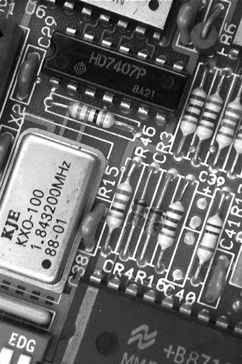
Figure 1.64 Conventional components mounted on a printed circuit board. Note that components such as C38, R46, etc. have leads that pass through holes in the printed circuit boards

Figure 1.65 Surface mounted components (note the appearance of capacitors C35, C52, and C53, and resistors, R87, R88, R91, etc.)
Solution
R88 will have a value of 1,000Ω (i.e., 10 followed by two zeros).
1.3 DC Circuits
In many cases, Ohm’s Law alone is insufficient to determine the magnitude of the voltages and currents present in a circuit. This section introduces several techniques that simplify the task of solving complex circuits. It also introduces the concept of exponential growth and decay of voltage and current in circuits containing capacitance and resistance and inductance and resistance. It concludes by showing how humble C-R circuits can be used for shaping the waveforms found in electronic circuits. We start by introducing two of the most useful laws of electronics.
1.3.1 Kirchhoff’s Laws
Kirchhoff’s Laws relate to the algebraic sum of currents at a junction (or node) or voltages in a network (or mesh). The term “algebraic” simply indicates that the polarity of each current or voltage drop must be taken into account by giving it an appropriate sign, either positive (+) or negative (−).
Kirchhoff’s Current Law states that the algebraic sum of the currents present at a junction (node) in a circuit is zero (see Figure 1.66).
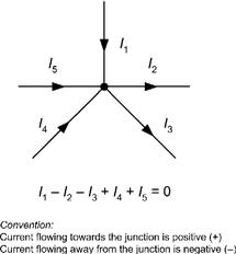
Figure 1.66 Kirchhoff’s Current Law

Solution
(a) I1 and I2 both flow toward Node A so, applying our polarity convention, they must both be positive. Now, assuming that a current I5 flows between A and B and that this current flows away from the junction (obvious because I1 and I2 both flow toward the junction), we arrive at the following Kirchhoff’s Current Law equation:
![]()
![]()
(b) Moving to Node B, let’s assume that I3 flows outward, so we can say that:
![]()
![]()
Kirchhoff’s Voltage Law states that the algebraic sum of the potential drops in a closed network (or “mesh”) is zero (see Figure 1.68).
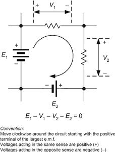
Figure 1.68 Kirchhoff’s Voltage Law

Solution
(a) In Loop A, and using the conventions shown in Figure 1.68, we can write down the Kirchhoff’s Voltage Law equations:
![]()
![]()
(b) Similarly, in Loop B, we can say that:
![]()
![]()
Example 1.61
Determine the currents and voltages in the circuit of Figure 1.70.

Figure 1.70 See Example 1.61
Solution
In order to solve the circuit shown in Figure 1.70, it is first necessary to mark the currents and voltages on the circuit, as shown in Figures 1.71 and 1.72.

Figure 1.71 See Example 1.61

Figure 1.72 See Example 1.61
By applying Kirchhoff’s Current Law at Node A that we’ve identified in Figure 1.70:
![]()
Therefore:
![]() (i)
(i)
By applying Kirchhoff’s Voltage Law in Loop A we obtain:
![]()
From which:
![]() (ii)
(ii)
By applying Kirchhoff’s Voltage Law in Loop B we obtain:
![]()
From which:
![]() (iii)
(iii)
Next we can generate three further relationships by applying Ohm’s Law:
and,

Combining these three relationships with the Current Law equation (i) gives:

![]()
Combining (ii) and (iii) with (iv) gives:
![]()
Multiplying both sides of the expression by 330 gives:
![]()
![]()
From which:
![]()
and:
![]()
From (ii):
![]()
From (iii):
![]()
Using the Ohm’s Law equations that we met earlier gives:
Finally, it’s worth checking these results with the Current Law equation (i):
![]()
Inserting our values for I1, I2 and I3 gives:
![]()
Since the left and right hand sides of the equation are equal we can be reasonably confident that our results are correct.
1.3.2 The Potential Divider
The potential divider circuit (see Figure 1.73) is commonly used to reduce voltages in a circuit. The output voltage produced by the circuit is given by:


Figure 1.73 Potential divider circuit
It is, however, important to note that the output voltage (Vout) will fall when current is drawn from the arrangement.
Figure 1.74 shows the effect of loading the potential divider circuit. In the loaded potential divider (Figure 1.74) the output voltage is given by:

where:

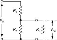
Figure 1.74 Loaded potential divider circuit
Example 1.62
The potential divider shown in Figure 1.75 is used as a simple voltage calibrator. Determine the output voltage produced by the circuit:

Figure 1.75 See Example 1.62

1.3.3 The Current Divider
The current divider circuit (see Figure 1.76) is used to divert a known proportion of the current flowing in a circuit. The output current produced by the circuit is given by:


Figure 1.76 Current divider circuit
It is, however, important to note that the output current (Iout) will fall when the load connected to the output terminals has any appreciable resistance.
Example 1.63
A moving coil meter requires a current of 1 mA to provide full-scale deflection. If the meter coil has a resistance of 100Ω and is to be used as a milliammeter reading 5 mA full-scale, determine the value of parallel shunt resistor required.
Solution
This problem may sound a little complicated so it is worth taking a look at the equivalent circuit of the meter (Figure 1.77) and comparing it with the current divider shown in Figure 1.76.

Figure 1.77 See Example 1.63
We can apply the current divider formula, replacing Iout with Im (the meter full-scale deflection current) and R2 with Rm (the meter resistance). R1 is the required value of shunt resistor, Rs, Hence:

Rearranging the formula gives:
![]()
thus,
![]()
![]()
from which,
![]()
So,

Now Iin = 1 mA, Rm = 100Ω and Iin = 5 mA, thus:
![]()
1.3.4 The Wheatstone Bridge
The Wheatstone bridge forms the basis of a number of useful electronic circuits including several that are used in instrumentation and measurement.
The basic form of Wheatstone bridge is shown in Figure 1.78. The voltage developed between A and B will be zero when the voltage between A and Y is the same as that between B and Y. In effect, R1 and R2 constitute a potential divider as do R3 and R4.

Figure 1.78 Basic Wheatstone bridge circuit
The bridge will be balanced (and VAB = 0) when the ratio of R1:R2 is the same as the ratio R3:R4.
Hence, at balance:

A practical form of Wheatstone bridge that can be used for measuring unknown resistances is shown in Figure 1.79.

Figure 1.79 See Example 1.64
In this practical form of Wheatstone bridge, R1 and R2 are called the ratio arms while one arm (that occupied by R3 in Figure 1.78) is replaced by a calibrated variable resistor. The unknown resistor, Rx, is connected in the fourth arm. At balance:

Example 1.64
A Wheatstone bridge is based on the circuit shown in Figure 1.79. If R1 and R2 can each be switched so that they have values of either 100Ω or 1 kΩ and RV is variable between 10Ω and 10 kΩ, determine the range of resistance values that can be measured.
Solution
The maximum value of resistance that can be measured will correspond to the largest ratio of R2:R1 (i.e., when R2 is 1 kΩ and R1 is 100Ω) and the highest value of RV (i.e., 10 kΩ). In this case:
![]()
The minimum value of resistance that can be measured will correspond to the smallest ratio of R2:R1 (i.e., when R1 is 100Ω and R1 is 1 kΩ) and the smallest value of RV (i.e., 10Ω). In this case:

Hence the range of values that can be measured extends from 1Ω to 100 kΩ.
1.3.5 Thévenin’s Theorem
Thévenin’s Theorem allows us to replace a complicated network of resistances and voltage sources with a simple equivalent circuit comprising a single voltage source connected in series with a single resistance (see Figure 1.70).
The single voltage source in the Thévenin equivalent circuit, Voc, is simply the voltage that appears between the terminals when nothing is connected to it. In other words, it is the open-circuit voltage that would appear between A and B.
The single resistance that appears in the Thévenin equivalent circuit, R, is the resistance that would be seen looking into the network between A and B when all of the voltage sources (assumed perfect) are replaced by short-circuit connections. Note that if the voltage sources are not perfect (i.e., if they have some internal resistance) the equivalent circuit must be constructed on the basis that each voltage source is replaced by its own internal resistance.
Once we have values for Voc and R, we can determine how the network will behave when it is connected to a load (i.e., when a resistor is connected across the terminals A and B).
Example 1.65
Figure 1.81 shows a Wheatstone bridge. Determine the current that will flow in a 100Ω load connected between terminals A and B.

Figure 1.80 Thévenin equivalent circuit

Figure 1.81 See Example 1.65
Solution
First we need to find the Thévenin equivalent of the circuit. To find Voc we can treat the bridge arrangement as two potential dividers.
The voltage across R2 will be given by:

Hence, the voltage at A relative to Y, VAY, will be 5.454V.
The voltage across R4 will be given by:

Hence, the voltage at B relative to Y, VBY, will be 4.444V.
The voltage VAB will be the difference between VAY and VBY. This, the open-circuit output voltage, VAB, will be given by:
![]()
Next we need to find the Thévenin equivalent resistance looking in at A and B. To do this, we can redraw the circuit, replacing the battery (connected between X and Y) with a short circuit, as shown in Figure 1.82.

Figure 1.82 See Example 1.65
The Thévenin equivalent resistance is given by the relationship:

From which:

The Thévenin equivalent circuit is shown in Figure 1.83. To determine the current in a 100Ω load connected between A and B, we can simply add a 100Ω load to the Thévenin equivalent circuit, as shown in Figure 1.84. By applying Ohm’s Law in Figure 1.84 we get:
![]()

Figure 1.83 Thévenin equivalent of Figure 1.81

Figure 1.84 Determining the current when the Thévenin equivalent circuit is loaded
1.3.6 Norton’s Theorem
Norton’s Theorem provides an alternative method of reducing a complex network to a simple equivalent circuit. Unlike Thévenin’s Theorem, Norton’s Theorem makes use of a current source rather than a voltage source. The Norton equivalent circuit allows us to replace a complicated network of resistances and voltage sources with a simple equivalent circuit comprising a single constant current source connected in parallel with a single resistance (see Figure 1.85).
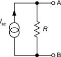
Figure 1.85 Norton equivalent circuit
The constant current source in the Norton equivalent circuit, Isc, is simply the short-circuit current that would flow if A and B were to be linked directly together. The resistance that appears in the Norton equivalent circuit, R, is the resistance that would be seen looking into the network between A and B when all of the voltage sources are replaced by short-circuit connections. Once again, it is worth noting that, if the voltage sources have any appreciable internal resistance, the equivalent circuit must be constructed on the basis that each voltage source is replaced by its own internal resistance.
As with the Thévenin equivalent, we can determine how a network will behave by obtaining values for Isc and R.
Example 1.66
Three temperature sensors having the following characteristics shown in Table 1.14 are connected in parallel as shown in Figure 1.86:
Table 1.14 Temperature sensor characteristics

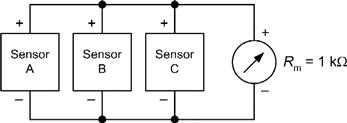
Figure 1.86 See Example 1.66
Determine the voltage produced when the arrangement is connected to a moving-coil meter having a resistance of 1 kΩ.
Solution
First we need to find the Norton equivalent of the circuit. To find Isc we can determine the short-circuit current from each sensor and add them together.
![]()
For sensor B:
![]()
For sensor C:
![]()
The total current, Isc, will be given by:
![]()
Next we need to find the Norton equivalent resistance. To do this, we can redraw the circuit showing each sensor replaced by its internal resistance, as shown in Figure 1.87.
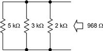
Figure 1.87 Determining the equivalent resistance in Figure 1.86
The equivalent resistance of this arrangement (think of this as the resistance seen looking into the circuit in the direction of the arrow shown in Figure 1.87) is given by:

where R1 = 5kΩ, R2 = 3kΩ, R3 = 2kΩ, hence:

![]()
from which:
![]()
The Norton equivalent circuit is shown in Figure 1.88. To determine the voltage in a 1 kΩ moving coil meter connected between A and B, we can make use of the Norton equivalent circuit by simply adding a 1 kΩ resistor to the circuit and applying Ohm’s Law, as shown in Figure 1.89.
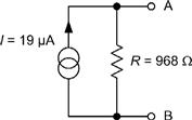
Figure 1.88 Norton equivalent of the circuit in Figure 1.86
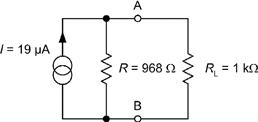
Figure 1.89 Determining the output voltage when the Norton equivalent circuit is loaded with 1 kΩ
The voltage appearing across the moving coil meter in Figure 1.90 will be given by:

hence:
![]()

Figure 1.90 The voltage drop across the meter is found to be 9.35 mV
1.3.7 C-R Circuits
Networks of capacitors and resistors (known as C-R circuits) form the basis of many timing and pulse shaping circuits and are thus often found in practical electronic circuits.
1.3.8 Charging
A simple C-R circuit is shown in Figure 1.91. In this circuit C is charged through R from the constant voltage source, Vs. The voltage, νc, across the (initially uncharged) capacitor voltage will rise exponentially as shown in Figure 1.92. At the same time, the current in the circuit, i, will fall, as shown in Figure 1.93.

Figure 1.91 A C-R circuit in which C is charged through R

Figure 1.92 Exponential growth of capacitor voltage, νc, in Figure 1.92

Figure 1.93 Exponential decay of current, i, in Figure 1.91
The rate of growth of voltage with time (and decay of current with time) will be dependent upon the product of capacitance and resistance. This value is known as the time constant of the circuit. Hence:
Time constant, t = C × R
where C is the value of capacitance (F), R is the resistance (F), and t is the time constant (s).
The voltage developed across the charging capacitor, νc, varies with time, t, according to the relationship:
![]()
where νc is the capacitor voltage, Vs is the DC supply voltage, t is the time, and CR is the time constant of the circuit (equal to the product of capacitance, C, and resistance, R).
The capacitor voltage will rise to approximately 63% of the supply voltage, Vs, in a time interval equal to the time constant.
At the end of the next interval of time equal to the time constant (i.e., after an elapsed time equal to 2CR) the voltage will have risen by 63% of the remainder, and so on. In theory, the capacitor will never become fully charged. However, after a period of time equal to 5CR, the capacitor voltage will to all intents and purposes be equal to the supply voltage. At this point, the capacitor voltage will have risen to 99.3% of its final value and we can consider it to be fully charged.
During charging, the current in the capacitor, i, varies with time, t, according to the relationship:
![]()
where Vs is the DC supply voltage, t is the time, R is the series resistance and C is the value of capacitance.
The current will fall to approximately 37% of the initial current in a time equal to the time constant. At the end of the next interval of time equal to the time constant (i.e., after a total time of 2CR has elapsed) the current will have fallen by a further 37% of the remainder, and so on.
Example 1.67
An initially uncharged 1 μF capacitor is charged from a 9V DC supply via a 3.3 MΩ resistor. Determine the capacitor voltage 1s after connecting the supply.
Solution
The formula for exponential growth of voltage in the capacitor is:
![]()
Here we need to find the capacitor voltage, νc, when Vs = 9V, t = 1s, C = 1 μF and R = 3.3 MΩ. The time constant, CR, will be given by:
![]()
Thus:
![]()
and,
![]()
Example 1.68
A 100 μF capacitor is charged from a 350V DC supply through a series resistance of 1 kΩ. Determine the initial charging current and the current that will flow 50 ms and 100 ms after connecting the supply. After what time is the capacitor considered to be fully charged?
Solution
At t = 0 the capacitor will be uncharged (νc = 0) and all of the supply voltage will appear across the series resistance. Thus, at t = 0:

When t = 50 ms, the current will be given by:
![]()
Where Vs = 350V, t = 50 ms, C = 100 μF, R = 1 kΩ. Hence:

When t = 100 ms (using the same equation but with t = 0.1s) the current is given by:

The capacitor can be considered to be fully charged when t = 5CR = 5 × 100 × 10−6 × 1 × 103 = 0.5s. Note that, at this point the capacitor voltage will have reached 99% of its final value.
Discharge
Having considered the situation when a capacitor is being charged, let’s consider what happens when an already charged capacitor is discharged.

Figure 1.94 C-R circuits are widely used in electronics. In this oscilloscope, for example, a rotary switch is used to select different C-R combinations in order to provide the various timebase ranges (adjustable from 500 ms/cm to 1 μs/cm). Each C-R time constant corresponds to a different timebase range.
When the fully charged capacitor from Figure 1.89 is connected as shown in Figure 1.95, the capacitor will discharge through the resistor, and the capacitor voltage, νC, will fall exponentially with time, as shown in Figure 1.96.
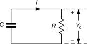
Figure 1.95 A C-R circuit in which C is initially charged and then discharges through R
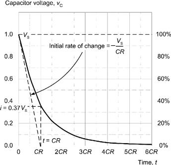
Figure 1.96 Exponential decay of capacitor voltage, νc, in Figure 1.95
The current in the circuit, i, will also fall, as shown in Figure 1.97. The rate of discharge (i.e., the rate of decay of voltage with time) will once again be governed by the time constant of the circuit, C × R.

Figure 1.97 Exponential decay of current, i, in Figure 1.95
The voltage developed across the discharging capacitor, νC, varies with time, t, according to the relationship:
![]()
where Vs, is the supply voltage, t is the time, C is the capacitance, and R is the resistance.
The capacitor voltage will fall to approximately 37% of the initial voltage in a time equal to the time constant. At the end of the next interval of time equal to the time constant (i.e., after an elapsed time equal to 2CR) the voltage will have fallen by 37% of the remainder, and so on.
In theory, the capacitor will never become fully discharged. However, after a period of time equal to 5CR, the capacitor voltage will to all intents and purposes be zero.
At this point the capacitor voltage will have fallen below 1% of its initial value. At this point we can consider it to be fully discharged.
As with charging, the current in the capacitor, i, varies with time, t, according to the relationship:
![]()
where Vs, is the supply voltage, t is the time, C is the capacitance, and R is the resistance.The current will fall to approximately 37% of the initial value of current, Vs/R, in a time equal to the time constant.
At the end of the next interval of time equal to the time constant (i.e., after a total time of 2CR has elapsed) the voltage will have fallen by a further 37% of the remainder, and so on.
Example 1.69
A 10 μF capacitor is charged to a potential of 20V and then discharged through a 47 kΩ resistor. Determine the time taken for the capacitor voltage to fall below 10V.
Solution
The formula for exponential decay of voltage in the capacitor is:
![]()
where Vs = 20V and CR = 10 μF × 47 kΩ = 0.47s.
We need to find t when νC = 10V. Rearranging the formula to make t the subject gives:

thus,

or,
![]()
In order to simplify the mathematics of exponential growth and decay, Table 1.15 provides an alternative tabular method that may be used to determine the voltage and current in a C-R circuit.
Table 1.15 Exponential growth and decay
| t/CR or t /(L/R) | k (growth) | k (decay) |
| 0.0 | 0.0000 | 1.0000 |
| 0.1 | 0.0951 | 0.9048 |
| 0.2 | 0.1812 | 0.8187 (1) |
| 0.3 | 0.2591 | 0.7408 |
| 0.4 | 0.3296 | 0.6703 |
| 0.5 | 0.3935 | 0.6065 |
| 0.6 | 0.4511 | 0.5488 |
| 0.7 | 0.5034 | 0.4965 |
| 0.8 | 0.5506 | 0.4493 |
| 0.9 | 0.5934 | 0.4065 |
| 1.0 | 0.6321 | 0.3679 |
| 1.5 | 0.7769 | 0.2231 |
| 2.0 | 0.8647 (2) | 0.1353 |
| 2.5 | 0.9179 | 0.0821 |
| 3.0 | 0.9502 | 0.0498 |
| 3.5 | 0.9698 | 0.0302 |
| 4.0 | 0.9817 | 0.0183 |
| 4.5 | 0.9889 | 0.0111 |
| 5.0 | 0.9933 | 0.0067 |
Notes: (1) See Example 1.70(2) See Example 1.74k is the ratio of the value at time, t, to the final value (e.g., νc/Vs)
Example 1.70
A 150 μF capacitor is charged to a potential of 150V. The capacitor is then removed from the charging source and connected to a 2 MΩ resistor. Determine the capacitor voltage 1 minute later.
Solution
We will solve this problem using Table 1.15 rather than the exponential formula.
First we need to find the time constant:
![]()
Next we find the ratio of t to CR:
After 1 minute, t = 60s therefore the ratio of t to CR is 60/300 or 0.2. Table 1.15 shows that when t/CR = 0.2, the ratio of instantaneous value to final value (k in Table 1.15) is 0.8187.
Thus,
![]()
or,
![]()
1.3.9 Waveshaping with C-R Networks
One of the most common applications of C-R networks is in waveshaping circuits. The circuits shown in Figures 1.98 and 1.100 function as simple square-to-triangle and square-to-pulse converters by, respectively, integrating and differentiating their inputs.

Figure 1.98 A C-R integrating circuit
The effectiveness of the simple integrator circuit shown in Figure 1.98 depends on the ratio of time constant, C × R, to periodic time, t. The larger this ratio is, the more effective the circuit will be as an integrator. The effectiveness of the circuit of Figure 1.98 is illustrated by the input and output waveforms shown in Figure 1.99.

Figure 1.99 Typical input and output waveforms for the integrating circuit shown in Figure 1.98
Similarly, the effectiveness of the simple differentiator circuit shown in Figure 1.100 also depends on the ratio of time constant C × R, to periodic time, t. The smaller this ratio is, the more effective the circuit will be as a differentiator.

Figure 1.100 A C-R differentiating circuit
The effectiveness of the circuit of Figure 1.100 is illustrated by the input and output waveforms shown in Figure 1.101.

Figure 1.101 Typical input and output waveforms for the integrating circuit shown in Figure 1.98
Example 1.71
A circuit is required to produce a train of alternating positive and negative pulses of short duration from a square wave of frequency 1 kHz. Devise a suitable C-R circuit and specify suitable values.
Solution
Here we require the services of a differentiating circuit along the lines of that shown in Figure 1.100. In order that the circuit operates effectively as a differentiator, we need to make the time constant, C × R, very much less than the periodic time of the input waveform (1 ms).
Assuming that we choose a medium value for R of, say, 10 kΩ, the maximum value which we could allow C to have would be that which satisfies the equation:
![]()
where R = 10 kΩ and t = 1 ms. Thus:
![]()
or,
![]()
In practice, any value equal or less than 10 nF would be adequate. A very small value (say less than 1 nF) will, however, generate pulses of a very narrow width.
Example 1.72
A circuit is required to produce a triangular waveform from a square wave of frequency 1 kHz. Devise a suitable C-R arrangement and specify suitable values.
Solution
This time we require an integrating circuit like that shown in Figure 1.98. In order that the circuit operates effectively as an integrator, we need to make the time constant, C × R, very much less than the periodic time of the input waveform (1 ms).
Assuming that we choose a medium value for R of, say, 10 kΩ, the minimum value which we could allow C to have would be that which satisfies the equation:
![]()
where R = 10 kΩ and t = 1 ms. Thus:
![]()
or,
![]()
In practice, any value equal or greater than 1 μF would be adequate. A very large value (say more than 10 μF) will, however, generate a triangular wave which has a very small amplitude. To put this in simple terms, although the waveform might be what you want there’s not a lot of it!
1.3.10 L-R Circuits
Networks of inductors and resistors (known as L-R circuits) can also be used for timing and pulse shaping. In comparison with capacitors, however, inductors are somewhat more difficult to manufacture and are consequently more expensive.
Inductors are also prone to losses and may also require screening to minimize the effects of stray magnetic coupling. Inductors are, therefore, generally unsuited to simple timing and waveshaping applications.
Figure 1.102 shows a simple L-R network in which an inductor is connected to a constant voltage supply. When the supply is first connected, the current, i, will rise exponentially with time, as shown in Figure 1.103. At the same time, the inductor voltage VL, will fall, as shown in Figure 1.104). The rate of change of current with time will depend upon the ratio of inductance to resistance and is known as the time constant. Hence:
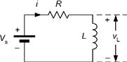
Figure 1.102 A C-R circuit in which C is initially charged and then discharges through R

Figure 1.103 Exponential growth of current, i, in Figure 1.102
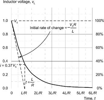
Figure 1.104 Exponential decay of voltage, νL, in Figure 1.102
Time constant, t = L/R
where L is the value of inductance (H), R is the resistance (Ω), and t is the time constant (s).
The current flowing in the inductor, i, varies with time, t, according to the relationship:
![]()
where Vs is the DC supply voltage, R is the resistance of the inductor, and L is the inductance.
The current, i, will initially be zero and will rise to approximately 63% of its maximum value (i.e., Vs/R) in a time interval equal to the time constant. At the end of the next interval of time equal to the time constant (i.e., after a total time of 2L/R has elapsed) the current will have risen by a further 63% of the remainder, and so on.
In theory, the current in the inductor will never become equal to Vs/R. However, after a period of time equal to 5L/R, the current will to all intents and purposes be equal to Vs/R. At this point, the current in the inductor will have risen to 99.3% of its final value.
The voltage developed across the inductor, νL, varies with time, t, according to the relationship:
![]()
where Vs is the DC supply voltage, R is the resistance of the inductor, and L is the inductance.
The inductor voltage will fall to approximately 37% of the initial voltage in a time equal to the time constant.
At the end of the next interval of time equal to the time constant (i.e., after a total time of 2L/R has elapsed) the voltage will have fallen by a further 37% of the remainder, and so on.
Example 1.73
A coil having inductance 6H and resistance 24Ω is connected to a 12V DC supply. Determine the current in the inductor 0.1s after the supply is first connected.
Solution
The formula for exponential growth of current in the coil is:
![]()
where Vs = 12V, L = 6H and R = 24Ω.
We need to find i when t = 0.1s
![]()
thus,
![]()
In order to simplify the mathematics of exponential growth and decay, Table 1.15 provides an alternative tabular method that may be used to determine the voltage and current in an L-R circuit.
Example 1.74
A coil has an inductance of l00 mH and a resistance of 10Ω. If the inductor is connected to a 5V DC supply, determine the inductor voltage 20 ms after the supply is first connected.
Solution
We will solve this problem using Table 1.15 rather than the exponential formula.
First we need to find the time constant:
![]()
Next we find the ratio of t to L/R.
When t = 20 ms the ratio of t to L/R is 0.02/0.01 or 2. Table 1.15 shows that when t/(L/R) = 2, the ratio of instantaneous value to final value (k) is 0.8647. Thus:
![]()
![]()
1.4 Alternating Voltage and Current
This section introduces basic alternating current theory. We discuss the terminology used to describe alternating waveforms and the behavior of resistors, capacitors, and inductors when an alternating current is applied to them. The chapter concludes by introducing another useful component, the transformer.
1.4.1 Alternating Versus Direct Current
Direct currents are currents which, even though their magnitude may vary, essentially flow only in one direction. In other words, direct currents are unidirectional. Alternating currents, on the other hand, are bidirectional and continuously reverse their direction of flow. The polarity of the e.m.f. which produces an alternating current must consequently also be changing from positive to negative, and vice versa.
Alternating currents produce alternating potential differences (voltages) in the circuits in which they flow. Furthermore, in some circuits, alternating voltages may be superimposed on direct voltage levels (see Figure 1.105). The resulting voltage may be unipolar (i.e., always positive or always negative) or bipolar (i.e., partly positive and partly negative).

Figure 1.105 (A) Bipolar sine wave; (B) unipolar sine wave (superimposed on a DC level)
1.4.2 Waveforms and Signals
A graph showing the variation of voltage or current present in a circuit is known as a waveform. There are many common types of waveform encountered in electrical circuits including sine (or sinusoidal), square, triangle, ramp or sawtooth (which may be either positive or negative going), and pulse.
Complex waveforms, like speech and music, usually comprise many components at different frequencies. Pulse waveforms are often categorized as either repetitive or nonrepetitive (the former comprises a pattern of pulses that repeats regularly while the latter comprises pulses which constitute a unique event). Some common waveforms are shown in Figure 1.106.

Figure 1.106 Common waveforms
Signals can be conveyed using one or more of the properties of a waveform and sent using wires, cables, optical and radio links. Signals can also be processed in various ways using amplifiers, modulators, filters, etc. Signals are also classified as either analog (continuously variable) or digital (based on discrete states).
1.4.3 Frequency
The frequency of a repetitive waveform is the number of cycles of the waveform which occur in unit time. Frequency is expressed in hertz (Hz) and a frequency of 1 Hz is equivalent to one cycle per second. Hence, if a voltage has a frequency of 400 Hz, 400 cycles of it will occur in every second.
The equation for the voltage shown in Figure 1.105(A) at a time, t, is:
![]()
while that in Figure 1.105(B) is:
![]()
where ν is the instantaneous voltage, Vmax is the maximum (or peak) voltage of the sine wave, VDC, is the DC offset (where present), and f is the frequency of the sine wave.
Example 1.75
A sine wave voltage has a maximum value of 20V and a frequency of 50 Hz. Determine the instantaneous voltage present (a) 2.5 ms and (b) 15 ms from the start of the cycle.
Solution
We can find the voltage at any instant of time using:
![]()
where Vmax = 20V and f = 50 Hz.
In (a), t = 2.5 ms, hence:
![]()
In (b), t = 15 ms, hence:
![]()
1.4.4 Periodic Time
The periodic time (or period) of a waveform is the time taken for one complete cycle of the wave (see Figure 1.107). The relationship between periodic time and frequency is thus:
![]()
where t is the periodic time (in s) and f is the frequency (in Hz).

Figure 1.107 One cycle of a sine wave voltage showing its periodic time
1.4.5 Average, Peak, Peak-Peak, and r.m.s. Values
The average value of an alternating current which swings symmetrically above and below zero will be zero when measured over a long period of time. Hence, average values of currents and voltages are invariably taken over one complete half-cycle (either positive or negative) rather than over one complete full-cycle (which would result in an average value of zero).
The amplitude (or peak value) of a waveform is a measure of the extent of its voltage or current excursion from the resting value (usually zero).
The peak-to-peak value for a wave which is symmetrical about its resting value is twice its peak value (see Figure 1.108).

Figure 1.108 One cycle of a sine wave voltage showing its peak and peak-peak values
The r.m.s. (or effective) value of an alternating voltage or current is the value which would produce the same heat energy in a resistor as a direct voltage or current of the same magnitude. Since the r.m.s. value of a waveform is very much dependent upon its shape, values are only meaningful when dealing with a waveform of known shape. Where the shape of a waveform is not specified, r.m.s. values are normally assumed to refer to sinusoidal conditions.
For a given waveform, a set of fixed relationships exist between average, peak, peak-peak, and r.m.s. values. The required multiplying factors are summarized for sinusoidal voltages and currents in Table 1.16.
Table 1.16 Multiplying factors for average, peak, peak-peak and r.m.s. values

Example 1.78
A sinusoidal voltage has an r.m.s. value of 240V. What is the peak value of the voltage?
Example 1.79
An alternating current has a peak-peak value of 50 mA. What is its r.m.s. value?
Example 1.80
A sinusoidal voltage 10V pk-pk is applied to a resistor of 1 kΩ What value of r.m.s. current will flow in the resistor?
Solution
This problem must be solved in two stages. First we will determine the peak-peak current in the resistor and then we shall convert this value into a corresponding r.m.s. quantity.
Since ![]() we can infer that:
we can infer that:
![]()
From which,

The required multiplying factor (peak-peak to r.m.s.) is 0.353. Thus:
![]()
1.4.6 Reactance
When alternating voltages are applied to capacitors or inductors the magnitude of the current flowing will depend upon the value of capacitance or inductance and on the frequency of the voltage. In effect, capacitors and inductors oppose the flow of current in much the same way as a resistor. The important difference being that the effective resistance (or reactance) of the component varies with frequency (unlike the case of a resistor where the magnitude of the current does not change with frequency).
1.4.7 Capacitive Reactance
The reactance of a capacitor is defined as the ratio of applied voltage to current and, like resistance, it is measured in Ohms. The reactance of a capacitor is inversely proportional to both the value of capacitance and the frequency of the applied voltage. Capacitive reactance can be found by applying the following formula:

where Xc is the reactance (in ohms), f is the frequency (in hertz), and C is the capacitance (in farads).
Capacitive reactance falls as frequency increases, as shown in Figure 1.109. The applied voltage, Vc, and current, Ic, flowing in a pure capacitive reactance will differ in phase by an angle of 90° or π/2 radians (the current leads the voltage). This relationship is illustrated in the current and voltage waveforms (drawn to a common time scale) shown in Figure 1.110 and as a phasor diagram shown in Figure 1.111.

Figure 1.109 Variation of reactance with frequency for a capacitor

Figure 1.110 Voltage and current waveforms for a pure capacitor (the current leads the voltage by 90°)
Figure 1.111 Phasor diagram for a pure capacitor
Solution
This problem is solved using the expression:
![]()
(a) At 100 Hz:
![]()
or,
![]()
(b) At 10 kHz:
![]()
or,
![]()
Example 1.82
A 100 nF capacitor is to form part of a filter connected across a 240V 50 Hz mains supply. What current will flow in the capacitor?
Solution
First we must find the reactance of the capacitor:
![]()
The r.m.s. current flowing in the capacitor will thus be:

1.4.8 Inductive Reactance
The reactance of an inductor is defined as the ratio of applied voltage to current and, like resistance, it is measured in ohms. The reactance of an inductor is directly proportional to both the value of inductance and the frequency of the applied voltage. Inductive reactance can be found by applying the formula:
![]()
where XL is the reactance in Ω, f is the frequency in Hz, and L is the inductance in H.
Inductive reactance increases linearly with frequency as shown in Figure 1.112. The applied voltage, VL, and current, IL, developed across a pure inductive reactance will differ in phase by an angle of 90° or π/2 radians (the current lags the voltage). This relationship is illustrated in the current and voltage waveforms (drawn to a common time scale) shown in Figure 1.113 and as a phasor diagram shown in Figure 1.114.

Figure 1.112 Variation of reactance with frequency for an inductor
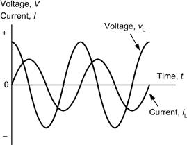
Figure 1.113 Voltage and current waveforms for a pure inductor (the voltage leads the current by 90°)
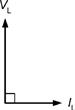
Figure 1.114 Phasor diagram for a pure inductor
Solution
(a) at 100 Hz:
![]()
(b) At 10 kHz:
![]()
Example 1.84
A 100 mH inductor of negligible resistance is to form part of a filter which carries a current of 20 mA at 400 Hz. What voltage drop will be developed across the inductor?
Solution
The reactance of the inductor will be given by:
![]()
The r.m.s. voltage developed across the inductor will be given by:
![]()
In this example, it is important to note that we have assumed that the DC resistance of the inductor is negligible by comparison with its reactance. Where this is not the case, it will be necessary to determine the impedance of the component and use this to determine the voltage drop.
1.4.9 Impedance
Figure 1.115 shows two circuits which contain both resistance and reactance. These circuits are said to exhibit impedance (a combination of resistance and reactance) which, like resistance and reactance, is measured in ohms.

Figure 1.115 (A) C and R in series (B) L and R in series (note that both circuits exhibit an impedance)
The impedance of the circuits shown in Figure 1.115 is simply the ratio of supply voltage, VS, to supply current, IS. The impedance of the simple C-R and L-R circuits shown in Figure 1.115 can be found by using the impedance triangle shown in Figure 1.116. In either case, the impedance of the circuit is given by:
![]()
and the phase angle (between VS and IS) is given by:
where Z is the impedance (in ohms), X is the reactance, either capacitive or inductive (expressed in ohms), R is the resistance (in ohms), and Φ is the phase angle in radians.

Figure 1.116 The impedance triangle
Example 1.85
A 2 μF capacitor is connected in series with a 100Ω resistor across a 115V 400 Hz AC supply. Determine the impedance of the circuit and the current taken from the supply.
1.4.10 Power Factor
The power factor in an AC circuit containing resistance and reactance is simply the ratio of true power to apparent power. Hence:
![]()
The true power in an AC circuit is the power which is actually dissipated in the resistive component. Thus:
![]()
The apparent power in an AC circuit is the power which is apparently consumed by the circuit and is the product of the supply current and supply voltage (note that this is not the same as the power which is actually dissipated as heat). Hence:
![]()
Hence:

From Figure 1.116,
![]()
Hence, the power factor of a series AC circuit can be found from the cosine of the phase angle.
Example 1.86
A choke (a form of inductor) having an inductance of 150 mH and resistance of 250Ω is connected to a 115V 400 Hz AC supply. Determine the power factor of the choke and the current taken from the supply.
Solution
First we must find the reactance of the inductor,
![]()
We can now determine the power factor from:
![]()
The impedance of the choke, Z, will be given by:
![]()
Finally, the current taken from the supply will be:
![]()
1.4.11 L-C Circuits
Two forms of L-C circuits are illustrated in Figure 1.117. Figure 1.117(A) is a series resonant circuit, while Figure 1.117(B) constitutes a parallel resonant circuit. The impedance of both circuits varies in a complex manner with frequency.

Figure 1.117 Series resonant and parallel resonant L-C and L-C-R circuits
The impedance of the series circuit in Figure 1.117(A) is given by:
![]()
where Z is the impedance of the circuit (in ohms), and XL and XC are the reactances of the inductor and capacitor respectively (both expressed in ohms).
The phase angle (between the supply voltage and current) will be +π/2 rad (i.e., +90°) when XL > XC (above resonance) or − π/2 rad (or −90°) when XC > XL (below resonance).
At a particular frequency (known as the series resonant frequency) the reactance of the capacitor, XC, will be equal in magnitude (but of opposite sign) to that of the inductor, XL. Due to this effective cancellation of the reactance, the impedance of the series resonant circuit will be zero at resonance. The supply current will have a maximum value at resonance (infinite in the case of a perfect series resonant circuit supplied from an ideal voltage source!).
The impedance of the parallel circuit in Figure 1.117B is given by:

where Z is the impedance of the circuit (in Ω), and XL and XC are the reactances of the inductor and capacitor, respectively (both expressed in Ω).
The phase angle (between the supply voltage and current) will be +π/2 rad (i.e., +90°) when XL > XC (above resonance) or π/2 rad (or −90°) when XC > XL (below resonance).
At a particular frequency (known as the parallel resonant frequency) the reactance of the capacitor, XC, will be equal in magnitude (but of opposite sign) to that of the inductor, XL. At resonance, the denominator in the formula for impedance becomes zero and thus the circuit has an infinite impedance at resonance. The supply current will have a minimum value at resonance (zero in the case of a perfect parallel resonant circuit).
1.4.12 L-C-R Circuits
Two forms of L-C-R network are illustrated in Figs 1.117(C) and 1.117(D); Figure 1.117(C) is series resonant while Figure 1.117(D) is parallel resonant. As in the case of their simpler L-C counterparts, the impedance of each circuit varies in a complex manner with frequency.
The impedance of the series circuit of Figure 1.117(C) is given by:
![]()
where Z is the impedance of the series circuit (in ohms), R is the resistance (in Ω), XL is the inductive reactance (in Ω) and XC is the capacitive reactance (also in Ω). At resonance the circuit has a minimum impedance (equal to R).
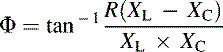
The phase angle (between the supply voltage and current) will be given by:

The impedance of the parallel circuit of Figure 1.117(D) is given by:

where Z is the impedance of the series circuit (in ohms), R is the resistance (in Ω), XL is the inductive reactance (in Ω) and XC is the capacitive reactance (also in Ω). At resonance the circuit has a minimum impedance (equal to R).
The phase angle (between the supply voltage and current) will be given by:
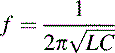
1.4.13 Resonance
The frequency at which the impedance is minimum for a series resonant circuit or maximum in the case of a parallel resonant circuit is known as the resonant frequency. The resonant frequency is given by:

where f0 is the resonant frequency (in hertz), L is the inductance (in henries) and C is the capacitance (in farads).
Typical impedance-frequency characteristics for series and parallel tuned circuits are shown in Figs 1.118 and 1.119.

Figure 1.118 Impedance versus frequency for a series L-C-R acceptor circuit

Figure 1.119 Impedance versus frequency for a parallel L-C-R rejector circuit
The series L-C-R tuned circuit has a minimum impedance at resonance (equal to R) and thus maximum current will flow. The circuit is consequently known as an acceptor circuit.
The parallel L-C-R tuned circuit has a maximum impedance at resonance (equal to R) and thus minimum current will flow. The circuit is consequently known as a rejector circuit.
1.4.14 Quality Factor
The quality of a resonant (or tuned) circuit is measured by its Q-factor. The higher the Q-factor, the sharper the response (narrower bandwidth), conversely the lower the Q-factor, the flatter the response (wider bandwidth), see Figure 1.120. In the case of the series tuned circuit, the Q-factor will increase as the resistance, R, decreases. In the case of the parallel tuned circuit, the Q-factor will increase as the resistance, R, increases. The response of a tuned circuit can be modified by incorporating a resistance of appropriate value either to “dampen” (low-Q) or “sharpen” (high-Q) the response. The relationship between bandwidth and Q-factor is:

where f2 and f1 are respectively the upper and lower cut-off (or half-power) frequencies (in Hertz), f0 is the resonant frequency (in hertz), and Q is the Q-factor (see Figure 1.121).
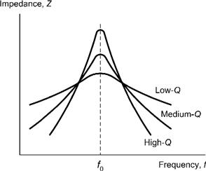
Figure 1.120 Effect of Q-factor on the response of a parallel resonant circuit (the response is similar, but inverted, for a series resonant circuit)

Figure 1.121 Bandwidth of a tuned circuit
Example 1.87
A parallel L-C circuit is to be resonant at a frequency of 400 Hz. If a 100 mH inductor is available, determine the value of capacitance required.
Solution
Rearranging the formula:
to make C the subject gives:

![]()
This value can be made from preferred values using a 2.2 μF capacitor connected in series with a 5.6 μF capacitor.
Example 1.88
A series L-C-R circuit comprises an inductor of 20 mH, a capacitor of 10 nF, and a resistor of 100Ω. If the circuit is supplied with a sinusoidal signal of 1.5V at a frequency of 2 kHz, determine the current supplied and the voltage developed across the resistor.
Solution
First we need to determine the values of inductive reactance, XL, and capacitive reactance XC:

The impedance of the series circuit can now be calculated:
![]()
From which:
![]()
The current flowing in the series circuit will be given by:
![]()
The voltage developed across the resistor can now be calculated using:
![]()
1.4.15 Transformers
Transformers provide us with a means of coupling AC power or signals from one circuit to another. Voltage may be stepped-up (secondary voltage greater than primary voltage) or stepped-down (secondary voltage less than primary voltage). Since no increase in power is possible (transformers are passive components like resistors, capacitors and inductors) an increase in secondary voltage can only be achieved at the expense of a corresponding reduction in secondary current, and vice versa (in fact, the secondary power will be very slightly less than the primary power due to losses within the transformer). Typical applications for transformers include stepping-up or stepping-down mains voltages in power supplies, coupling signals in AF amplifiers to achieve impedance matching and to isolate DC potentials associated with active components.
The electrical characteristics of a transformer are determined by a number of factors including the core material and physical dimensions. The specifications for a transformer usually include the rated primary and secondary voltages and current the required power rating (i.e., the maximum power, usually expressed in volt-amperes, VA) which can be continuously delivered by the transformer under a given set of conditions, the frequency range for the component (usually stated as upper and lower working frequency limits), and the regulation of a transformer (usually expressed as a percentage of full-load). This last specification is a measure of the ability of a transformer to maintain its rated output voltage under load.
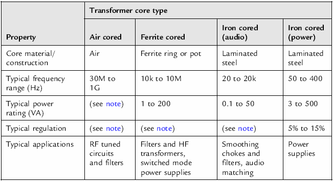
Table 1.17 summarizes the properties of three common types of transformer. Figure 1.124 shows the construction of a typical iron-cored power transformer.
Table 1.17 Characteristics of common types of transformers
1.4.16 Voltage and Turns Ratio
The principle of the transformer is illustrated in Figure 1.125. The primary and secondary windings are wound on a common low-reluctance magnetic core. The alternating flux generated by the primary winding is therefore coupled into the secondary winding (very little flux escapes due to leakage). A sinusoidal current flowing in the primary winding produces a sinusoidal flux. At any instant the flux in the transformer is given by the equation:
![]()
where Φmax is the maximum value of flux (in webers), f is the frequency of the applied current (in hertz), and t is the time in seconds.

Figure 1.122 A selection of transformers with power ratings from 0.1 VA to 100 VA

Figure 1.123 Parts of a typical iron-cored power transformer prior to assembly
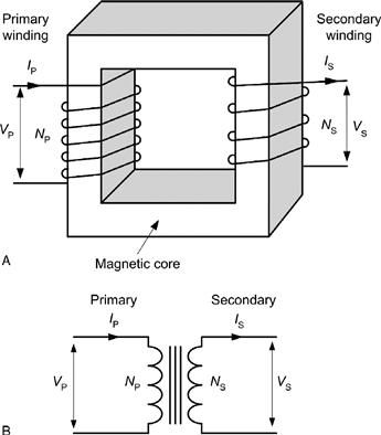

Figure 1.124 Construction of a typical iron-cored transformer
Figure 1.125 The transformer principle
The r.m.s. value of the primary voltage, VP, is given by:
![]()
Similarly, the r.m.s. value of the secondary voltage, VS, is given by:
![]()
Now:

where NP/NS is the turns ratio of the transformer.
Assuming that the transformer is loss-free, primary and secondary powers (PP and PS, respectively) will be identical. Hence:
![]()
Hence,

Finally, it is sometimes convenient to refer to a turns-per-volt rating for a transformer. This rating is given by:

Example 1.89
A transformer has 2,000 primary turns and 120 secondary turns. If the primary is connected to a 220V r.m.s. AC mains supply, determine the secondary voltage.
Solution
Rearranging:

gives:

Example 1.90
A transformer has 1,200 primary turns and is designed to operate with a 200V AC supply. If the transformer is required to produce an output of 10V, determine the number of secondary turns required. Assuming that the transformer is loss-free, determine the input (primary) current for a load current of 2.5A.

Figure 1.126 Resonant air-cored transformer arrangement. The two inductors are tuned to resonance at the operating frequency (145 MHz) by means of the two small preset capacitors
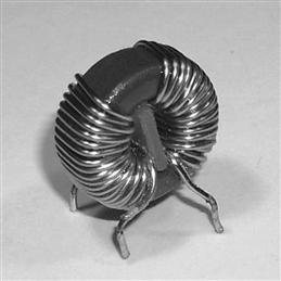
Figure 1.127 This small 1:1 ratio toroidal transformer forms part of a noise filter connected in the input circuit of a switched mode power supply. The transformer is wound on a ferrite core and acts as a choke, reducing the high-frequency noise that would otherwise be radiated from the mains supply wiring


1.5 Circuit Simulation
Computer simulation provides you with a powerful and cost-effective tool for designing, simulating, and analyzing a wide variety of electronic circuits. In recent years, the computer software packages designed for this task have not only become increasingly sophisticated but also have become increasingly easy to use. Furthermore, several of the most powerful and popular packages are now available at low cost either in evaluation, “lite” or student versions. In addition, there are several excellent freeware and shareware packages.
Whereas early electronic simulation software required that circuits were entered using a complex netlist that described all of the components and connections present in a circuit, most modern packages use an on-screen graphical representation of the circuit on test. This, in turn, generates a netlist (or its equivalent) for submission to the computational engine that actually performs the circuit analysis using mathematical models and algorithms. In order to describe the characteristics and behavior of components such as diodes and transistors, manufacturers often provide models in the form of a standard list of parameters.

Figure 1.128 Using Tina Pro to construct and test a circuit prior to detailed analysis
Most programs that simulate electronic circuits use a set of algorithms that describe the behavior of electronic components. The most commonly used algorithm was developed at the Berkeley Institute in the United States and it is known as SPICE (Simulation Program with Integrated Circuit Emphasis).
Results of circuit analysis can be displayed in various ways, including displays that simulate those of real test instruments (these are sometimes referred to as virtual instruments). A further benefit of using electronic circuit simulation software is that, when a circuit design has been finalized, it is usually possible to export a file from the design/simulation software to a PCB layout package. It may also be possible to export files for use in screen printing or CNC drilling. This greatly reduces the time that it takes to produce a finished electronic circuit.
1.5.1 Types of Analysis
Various types of analysis are available within modern SPICE-based circuit simulation packages. These usually include:
1.5.1.1 DC Analysis
DC analysis determines the DC operating point of the circuit under investigation. In this mode any wound components (e.g., inductors and transformers) are short-circuited and any capacitors that may be present are left open-circuit. In order to determine the initial conditions, a DC analysis is usually automatically performed prior to a transient analysis. It is also usually performed prior to an AC small-signal analysis in order to obtain the linearized, small-signal models for nonlinear devices. Furthermore, if specified, the DC small-signal value of a transfer function (ratio of output variable to input source), input resistance, and output resistance is also computed as a part of the DC solution. The DC analysis can also be used to generate DC transfer curves in which a specified independent voltage or current source is stepped over a user-specified range and the DC output variables are stored for each sequential source value.
1.5.1.2 AC Small-Signal Analysis
The AC small-signal analysis feature of SPICE software computes the AC output variables as a function of frequency. The program first computes the DC operating point of the circuit and determines linearized, small-signal models for all of the nonlinear devices in the circuit (e.g., diodes and transistors). The resultant linear circuit is then analyzed over a user-specified range of frequencies. The desired output of an AC small-signal analysis is usually a transfer function (voltage gain, transimpedance, etc.). If the circuit has only one AC input, it is convenient to set that input to unity and zero phase, so that output variables have the same value as the transfer function of the output variable with respect to the input.
1.5.1.3 Transient Analysis
The transient analysis feature of a SPICE package computes the transient output variables as a function of time over a user-specified time interval. The initial conditions are automatically determined by a DC analysis. All sources that are not time dependent (for example, power supplies) are set to their DC value.

Figure 1.129 An astable multivibrator circuit being simulated using B2 Spice
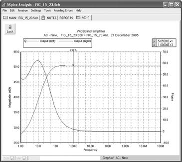

Figure 1.130 A Class B push-pull amplifier circuit being simulated by Multisim
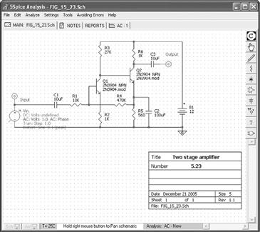
Figure 1.131 High-gain amplifier being analyzed using the 5Spice Analysis package
Figure 1.132 Gain and phase plotted as a result of small-signal AC analysis of the circuit in Figure 1.131

Figure 1.133 High-gain amplifier being analyzed using the Tina Pro package
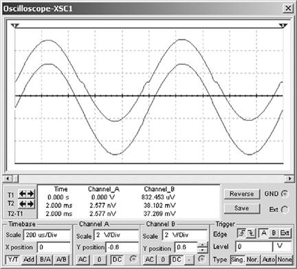

Figure 1.134 Gain and phase plotted as a result of small-signal AC analysis of the circuit in Figure 1.133
1.5.1.4 Pole-zero Analysis
The pole-zero analysis facility computes the poles and/or zeros in the small-signal AC transfer function. The program first computes the DC operating point and then determines the linearized, small-signal models for all the nonlinear devices in the circuit. This circuit is then used to find the poles and zeros of the transfer function.

Figure 1.135 Results of DC analysis of the circuit shown in Figure 1.133
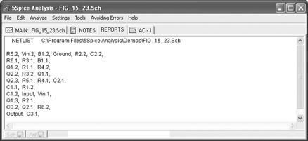
Figure 1.136 Computer generated netlist for the circuit shown in Figure 1.131

Figure 1.137 Results of AC analysis of the circuit shown in Figure 1.133
Two types of transfer functions are usually supported. One of these determines the voltage transfer function (i.e., output voltage divided by input voltage) and the other usually computes the output transimpedance (i.e., output voltage divided by input current) or transconductance (i.e., output current divided by input voltage). These two transfer functions cover all the cases and one can make it possible to determine the poles/zeros of functions like impedance ratio (i.e., input impedance divided by output impedance) and voltage gain. The input and output ports are specified as two pairs of nodes. Note that, for complex circuits it can take some time to carry out this analysis and the analysis may fail if there is an excessive number of poles or zeros.
1.5.1.5 Small-Signal Distortion Analysis
The distortion analysis facility provided by SPICE-driven software packages computes steady-state harmonic and inter-modulation products for small input signal magnitudes. If signals of a single frequency are specified as the input to the circuit, the complex values of the second and third harmonics are determined at every point in the circuit. If there are signals of two frequencies input to the circuit, the analysis finds out the complex values of the circuit variables at the sum and difference of the input frequencies, and at the difference of the smaller frequency from the second harmonic of the larger frequency.
1.5.1.6 Sensitivity Analysis
Sensitivity analysis allows you to determine either the DC operating-point sensitivity or the AC small-signal sensitivity of an output variable with respect to all circuit variables, including model parameters. The software calculates the difference in an output variable (either a node voltage or a branch current) by perturbing each parameter of each device independently. Since the method is a numerical approximation, the results may demonstrate second order affects in highly sensitive parameters, or may fail to show very low but nonzero sensitivity. Further, since each variable is perturbed by a small fraction of its value, zero-valued parameters are not analyzed (this has the benefit of reducing what is usually a very large amount of data).
1.5.1.7 Noise Analysis
The noise analysis feature determines the amount of noise generated by the components and devices (e.g., transistors) present in the circuit that is being analyzed. When provided with an input source and an output port, the analysis calculates the noise contributions of each device (and each noise generator within the device) to the output port voltage. It also calculates the input noise to the circuit, equivalent to the output noise referred to the specified input source. This is done for every frequency point in a specified range. After calculating the spectral densities, noise analysis integrates these values over the specified frequency range to arrive at the total noise voltage/current (over this frequency range).
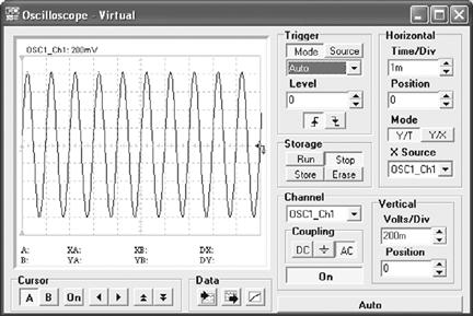
Figure 1.138 Using the virtual oscilloscope in Tina Pro to display the output voltage waveform for the circuit shown in Figure 1.133
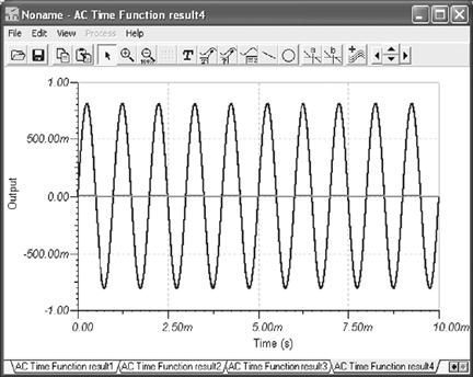
Figure 1.139 Alternative waveform plotting facility provided in Tina Pro
1.5.1.8 Thermal Analysis
Many SPICE packages will allow you to determine the effects of temperature on the performance of a circuit. Most analyses are performed at normal ambient temperatures (e.g., 27°C) but it can be advantageous to look at the effects of reduced or increased temperatures, particularly where the circuit is to be used in an environment in which there is a considerable variation in temperature.

Figure 1.140 Analysis of a Wien Bridge oscillator using B2 Spice.

Figure 1.141 Transient analysis of the circuit in Figure 1.140 produced the output waveform plot
1.5.2 Netlists and Component Models
The following is an example of how a netlist for a simple differential amplifier is constructed (note that the line numbers have been included solely for explanatory purposes):
Lines 2 and 3 define the supply voltages. VCC is +12V and is connected between node 7 and node 0 (signal ground). VEE is −12V and is connected between node 8 and node 0 (signal ground). Line 4 defines the input voltage which is connected between node 1 and node 0 (ground) while lines 5 and 6 define 1 kΩ resistors (RS1 and RS2) connected between 1 and 2, and 6 and 0.
Lines 7 and 8 are used to define the connections of two transistors (Q1 and Q2). The characteristics of these transistors (both identical) are defined by MOD1 (see line 12). Lines 9, 10 and 11 define the connections of three further resistors (RC1, RC2 and RE respectively). Line 12 defines the transistor model. The device is NPN and has a current gain of 50. The corresponding circuit is shown in Figure 1.142.

Figure 1.142 Differential amplifier with the nodes marked for generating a netlist
Most semiconductor manufacturers provide detailed SPICE models for the devices that they produce. The following is a manufacturer’s SPICE model for a 2N3904 transistor:
NPN (Is = 6.734f Xti = 3 Eg = 1.11 Vaf = 74.03 Bf = 416.4 Ne = 1.259 Ise = 6.734 Ikf = 66.78m Xtb = 1.5 Br = .7371 Nc = 2 Isc = 0 Ikr = 0 Rc = 1 Cjc = 3.638p Mjc = .3085 Vjc = .75 Fc = .5 Cje = 4.493p Mje = .2593 Vje = .75 Tr = 239.5n Tf = 301.2p Itf = .4 Vtf = 4 Xtf = 2 Rb = 10)
1.5.3 Logic Simulation
As well as an ability to carry out small-signal AC and transient analysis of linear circuits (see Figure 1.130 and 1.143), modern SPICE software packages usually incorporate facilities that can be used to analyze logic and also “mixed-mode” (i.e., analog and digital) circuits. Several examples of digital logic analysis are shown in Figures 1.144, 1.145 and 1.146.
Figure 1.143 Cross-over distortion evident in the output waveform from the Class B amplifier shown in Figure 1.130
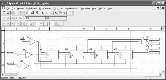
Figure 1.144 Four-stage circulating shift register simulated using B2 Spice

Figure 1.145 Waveforms for the four stage circulating shift register in Figure 1.144

Figure 1.146 Using B2 Spice to check the function of a simple combinational logic circuit
Figure 1.144 shows a four-stage shift register based on J-K bistables. The result of carrying out an analysis of this circuit is shown in Figure 1.145.
Finally, Figure 1.146 shows how a simple combinational logic circuit can be rapidly “assembled” and tested and its logical function checked. This circuit arrangement shows how the exclusive-OR function can be realized using only two-input NAND gates.
1.6 Intuitive Circuit Design
Mechanical engineers have it easy. They can see what they are working on most of the time. As an EE, you do not usually have that luxury. You have to imagine how those pesky electrons are flittering around in your circuit. We are going to cover some basic comparisons that use things you are familiar with to create an intuitive understanding of a circuit. As a side benefit, you will be able to hold your own in a mechanical discussion as well. There are several reasons to do this:
• The typical person understands the physical world more intuitively than they understand the electrical one. This is because we interact with it using all of our senses, whereas the electrical world is still very magical, even to an educated engineer. This is because much of what happens inside a circuit cannot be seen, felt, or heard. Think about it. You flip on a light switch and the light goes on. You really don’t consider how the electricity caused it to happen. Drag a heavy box across the floor, and you certainly understand the principle of friction.
• The rules for both disciplines are exactly the same. Once you understand one, you will understand the other. This is great, because you only have to learn the principles once. When you get a feel for what is happening inside a circuit, you can be an amazingly accurate troubleshooter. The human mind is an incredible instrument for simulation and, unlike a computer, it can make intuitive leaps to correct conclusions based on incomplete information. I believe that by learning these similarities you increase your mind’s ability to put together clues to the operation and results of a given system, resulting in correct analysis. This will help your mind to “simulate” a circuit.
1.6.1 Physical Equivalents of Electrical Components
Before we move on to the physical equivalents, let’s understand voltage, current and power. Voltage is the potential of the electron flow. Current is the amount of flow. Sometimes the best analogies are the old overused ones and that is true in this case. Think of it in terms of water in a squirt gun. Voltage is the amount of pressure in the gun. Pressure determines how far the water squirts, but a little pea shooter with a 30-foot shot and a dinky little stream won’t get you soaked. Current is the size of the water stream, but a large stream that doesn’t shoot far is not much help in a water fight. Voltage, current and power in electrical terms are related the same way. It is in fact a simple relationship; here is the equation:
![]() (1.1)
(1.1)
To get power you need both voltage and current. If either one of these are zero, you get zero power output. Let’s discuss three basic components and look at how they relate to voltage and current.
1.6.2 The Resistor is Analogous to Friction
Think about what happens when you drag a heavy box across the floor. A force called friction resists the movement of the box. This friction is related to the speed of the box. The faster you try to move the box, the more the friction resists your work. It can be described by an equation.
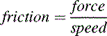 (1.2)
(1.2)

Figure 1.147 Friction resists smiley stick boy’s efforts
Furthermore, the friction dissipates the energy loss in the system with heat. Let me rephrase that. Friction makes things get warm. Don’t believe me? Try rubbing your hands together right now. Did you feel the heat? That is caused by friction. The function of a resistor in an electrical circuit is equal to friction. The resistor resists the flow of electricity just like friction resists the speed of the box. And, guess what, it heats up as it does so. An equation called Ohm’s Law describes this relationship:
![]() (1.3)
(1.3)
Do you see the similarity to the friction equation? They are exactly the same. The only real difference is the units you are working in.
1.6.3 The Inductor is Analogous to Mass
Let’s stay with the box example for now. First let’s eliminate friction, so as not to cloud our comprehension. The box is on a smooth track with virtually frictionless wheels. You notice that it takes some work to get the box going, but once moving, it coasts along nicely. In fact, it takes work to get it to stop again. How much work depends on how heavy the box is. This is known as the law of inertia. Newton postulated this long before electricity was discovered, but it applies very well to inductance. Mass resists a change in speed. Correspondingly, inductance resists a change in current.
 (1.4)
(1.4)
![]() (1.5)
(1.5)
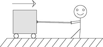
Figure 1.148 Wheels eliminate friction but smiley has a hard time getting it up to speed and stopping
1.6.4 The capacitor is analogous to a spring
So what does a spring do? Take hold of a spring in your mind’s eye. Stretch it out and hold it, and then let it go. What happens? It snaps back into position. A spring has a capacity to store energy. When a force is applied, it will hold that energy till it is released. Capacitance is similar to the elasticity of the spring. (One note: the spring constant that you may remember from physics texts is the inverse of the elasticity.) I always thought it was nice that the word capacitor is used to represent a component that has the capacity to store energy. (Technically an inductor can store energy too. In a capacitor the energy is stored in the electric field that is generated in and around the cap; in an inductor energy is stored in the magnetic field that is generated. This energy stored in an inductor can be tapped very efficiently at high currents. That is why most switching power supplies have an inductor in them as the primary passive component.)
 (1.6)
(1.6)
 (1.7)
(1.7)
1.6.5 A Tank Circuit
Take the basic tank or LC circuit. What does it do? It oscillates. A perfect circuit would go on forever at the resonant frequency. How should this appear in our mechanical circuit? Think about the equivalents: an inductor and a capacitor, a spring and mass. In a thought experiment, hook the spring up to the box from the previous drawing. Now give it a tug. What happens? It oscillates.

Figure 1.149 Get this started and it will keep bouncing until friction brings it to a halt
1.6.6 A Complex Circuit
Let’s follow this reasoning for an LCR circuit. All we need to do is add a little resistance, or friction, to the mass-spring of the tank circuit. Let’s tighten the wheels on our box a little too much so that they rub. What will happen after you give the box a tug? It will bounce back and forth a bit till it comes to a stop. The friction in the wheels slows it down. This friction component is called a damper, because it dampens the oscillation. What is it that a resistor does to an LC circuit? It dampens the oscillation.
There you have it, the world of electricity reduced to everyday items. Since these components are so similar, all the math tricks you may have learned apply as well to one system as they do to the other. Remember Fourier’s theorems? They were discovered for mechanical systems long before anyone realized that they work for electrical circuits as well. Remember all that higher math you used to know or are just now learning about—Laplace transforms, integrals, derivatives, etc.? It all works the same in both worlds. You can solve a mechanical system using Laplace methods just the same as an electrical circuit.
Back in the ’50s and ’60s, the government spent mounds of dough using electrical circuits to model physical systems as described above. Why? You can get into all sorts of integrals, derivatives and other ugly math when modeling real-world systems. All that can get jumbled quickly after a couple of orders of complexity. Think about an artillery shell fired from a tank. How do you predict where it will land? You have the friction of the air, the mass of the shell, the spring of the recoil. Instead of trying to calculate all that math by hand, you can build a circuit with all the various electrical components representing the mechanical ones, hook up an oscilloscope, and fire away. If you want to test 1000 different weights of artillery at different altitudes, electrons are much cheaper than gunpowder.
1.6.7 Learn an Intuitive Approach
1.6.7.1 Intuitive Signal Analysis
I’m not sure if this is actually taught in school. This is my name for it. It is something I learned on my own in college and the workplace. I didn’t call it an actual discipline until I had been working for a while and had explained my methods to fellow engineers to help them solve their own dilemmas. I do think, however, that a lot of so-called bright people out there use this skill without really knowing it or putting a name to it. They seem to be able to point to something you have been working on for hours and say “your problem is there.” They just seem to know intuitively what should happen. I believe this is a skill that can and should be taught.
There are three underlying principles needed to apply intuitive signal analysis. (Let’s just call it ISA. After all, if I have any hope of this catching on in the engineering world, it has to have an acronym!)
First, you must drill the basics. For example, what happens to the impedance of a capacitor as frequency increases? It goes down. You should know that type of information off the top of your head. If you do, you can identify a high-pass or low-pass filter immediately. How about the impedance of an inductor—what does it do as frequency increases? What does negative feedback do to an op-amp, how does its output change? You do not necessarily need to know every equation by heart, but you do need to know direction of the change. As far as the magnitude of the change is concerned, if you have a general idea of the strength of the signal that is usually enough to zero in on the part of the circuit that is not doing what you want it to.
Second, you need experience and lots of it. You need to get a feel for how different components work. You need to spend a lot of time in the lab and you need to understand the basics of each component. You need to know what a given signal will do as it passes through a given component. Remember the physical equivalents of the basic components? These are the building blocks of your ability to visualize the operation of a circuit. You must imagine what is happening inside the circuit as the input changes. If you can visualize that, you can predict what the outputs will do.
Third, break the problem down. “How do you eat an elephant?” the knowledge seeker asked the wise old man. “One bite at a time,” he replied. Pick a point to start and walk though it. Take the circuit and break it down into smaller chunks that can be handled easily. Draw arrows step by step that show the changes of signals in the circuit. “Does current go up here?” “Voltage at such and such point should be going down.” These are the types of questions and answers you should be mumbling to yourself. Again, one thing you do not need to know is what the output will be precisely. You do not need to memorize every equation in the book to intuitively know your circuit, but you do need to know what effect changing a value of a component will have. For example, given a low-pass RC filter and an AC signal input, if you increase the value of the capacitor, what should happen to the amplitude of the output? Will it get smaller or larger? You should know immediately with something this basic that the answer is “smaller.” You should also know that how much smaller depends on the frequency of the signal and the time constant of the filter. What happens as you increase current into the base of a transistor? Current through the collector increases. What happens to voltage across a resistor as current decreases? These are simple effects of components, but you would be surprised at how many engineers don’t know the answers to these types of questions off the top of their head.
Spending a lot of time in the lab will help immensely to develop this skill. If you look at the response of a lot of different circuits many, many times, you will learn how they should act. When this knowledge is integrated, a wonderful thing happens. Your head becomes a circuit simulator. You will be able to sum up the effects caused by the various components in the circuit and intuitively understand what is happening. Let me show you an example.
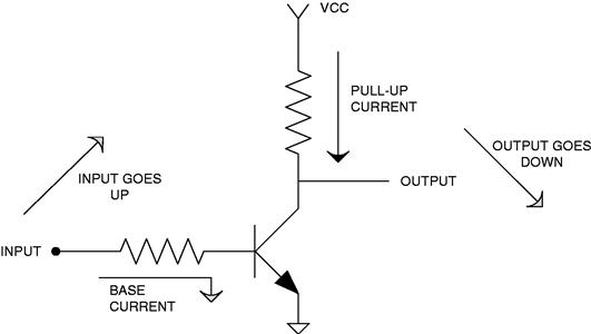
Figure 1.150 Use arrows to visualize what is happening to voltage and current
Now at this time you may not have a clue as to what a transistor is, so you may need to file this example away until you get past the transistor chapter, but be sure to come back to it so that the “Aha!” light bulb clicks on over your head. The analysis idea is what I am trying to get across, as you need it early on, but it creates a type of chicken-and-egg dilemma when it comes to an example. So for now, consider this example with the knowledge that the transistor is a device that moves current through the output that is proportional to the current through the base.
As voltage at the input above increases, base current increases. This causes the pullup current to increase, resulting in a larger voltage drop across the pull-up resistor. This means the voltage at the output must go down as the voltage at the input goes up. That is an example of putting it all together to really understand how a circuit works.
One way to develop this intuitive understanding is by use of computer simulators. It is easy to change a value and see what effect it has on the output and you can try several different configurations in a short amount of time. However, you have to be careful with these tools. It is easy to fall into a common trap, trusting the simulator so much that you will think there is something wrong with the real world when it doesn’t work right in the lab. The real world is not at fault! It is the simulator that is missing something. I think it is best for the engineer to begin using simulators to model simple circuits. Don’t jump into a complex model until you grasp what the basic components do—for example, modeling a step input into a RC circuit. With a simple model like this, change the values of R and C to see what happens. This is one way an engineer can develop the correct intuitive understanding of these two components. One word of warning though—don’t spend all your time on the simulator. Make sure you get some good bench time too.
You will find this signal analysis skill very useful in diagnosing problems as well as in your design efforts. As your intuitive understanding increases, you will be able to leap to correct conclusions without all the necessary facts. You will know when you are modeling something incorrectly because the result just doesn’t look right. Intuition is a skill no computer has, so make sure you take advantage of it!
Thumb Rules
• Drill the basics; know the basic formulas by heart.
• Get a lot of experience with basic circuits; the goal is to intuitively know how a signal will be affected by a component. Spend a lot of time on the bench!
• Break the problem down; draw arrows and notes on the schematic that indicate what the signal is doing.
• Determine what direction the signal is going; is it inversely related or directly related?
• Develop estimation abilities.
• Spend time on the bench with a scope and simple components.
1.6.8 “Lego” Engineering
1.6.8.1 Building Blocks
OK, so I came up with a fourth item. One of my instructors taught me a secret that I would like to pass on. Almost every discipline is easier to understand than you might think. The secret professors don’t want you to know is there are usually about five or six basic principles or equations that lie at the bottom of the pile, so to speak. These fundamentals, once they are grasped, will allow you to derive the rest of the principles or equations in that field. They are like the old simple Legos®; you had five or six shapes to make everything. If you truly understand these few basic fundamentals in a given discipline, you will excel in that discipline. One other thing this instructor often said was that all the great discoveries were only one or two levels above these fundamentals. This means if you really know the basics well, you will excel at the rest. One thing you can be sure of is the human tendency to forget. All the higher level stuff is often left unused and will quickly be forgotten, but even an engineer-turned-manager like me uses the basics nearly every day.
Since this is a book on electrical engineering, let’s list the fundamental equations for electrical circuits as I see them:
• Capacitors impede changes in voltage
• Inductors impede changes in current
Let me touch on a couple of examples. You may say, “You didn’t even list series and parallel capacitors. Isn’t that a basic rule?” Well, you are right, it is fairly basic but it really isn’t at the bottom of the pile. Series and parallel resistors are even more fundamental, because all that really happens when you add in the caps is the frequency of the signal is taken into account, other than that it is exactly the same equation! You would be better served to understand how a capacitor or inductor works and apply it to the basics than try to memorize too many equations. “What about Norton’s theorem?” you might ask. Bottom line, it is just the flip side of Thevenin’s theorem, so why learn two when one will do? I prefer to think of it terms of voltage so I set this to memory. You could work in terms of current and use Norton’s theorem, but you would arrive at the same answer at the end of the day. So pick one and go with it.
You can always look the more advanced stuff up, but most of the time a solid application of the basics will force the problem at hand to submit to your engineering prowess. These six rules are things that you should memorize, understand and be able to do approximations of in your head. These are the rules that will make the intuition you are developing a powerful tool. It will unleash the simulation capability that you have right in your own brain.
If you really take this advice to heart, years down the road when you’ve advance to “management” and you have forgotten all the advanced stuff you used to know, you will still be able to solve engineering problems to the amazement of your engineers.
This can be generalized to all disciplines. Look at what you are trying to learn, figure out the few basic points being made from which you can derive the rest, and you will have discovered the basic “Legos” for that subject. Those are what you should know forward and backward to succeed in that field. Besides, Legos are fun, aren’t they?
1.7 Troubleshooting Basics
1.7.1 If Only Everything Would Always Go Right…
Why are we interested in troubleshooting? Because even the best engineers take on projects whose requirements are so difficult and challenging that the circuits don’t work as expected—at least not the first time. I don’t have data on switching regulators, but I read in an industry study that when disk drives are manufactured, the fraction that fails to function when power is first applied typically ranges from 20 to 70%. Of course, this fraction may occasionally fall as low as 1% and rise as high as 100%. But, on the average, production engineers and technicians must be prepared to repair 20, 40, or 60% of these complex units. Switching-regulated power supplies can also be quite complex. If you manufacture them in batches of 100, you shouldn’t be surprised to find some batches with 12 pieces that require troubleshooting and other batches that have 46 such pieces. The troubleshooting may, as you well know, be tough with a new product whose bugs haven’t been worked out. But it can be even tougher when the design is old and the parts it now uses aren’t quite like the ones you used to be able to buy. Troubleshooting can be tougher still when there isn’t much documentation describing how the product is supposed to work, and the designer isn’t around any more. If there’s ever a time when troubleshooting isn’t needed, it’s just a temporary miracle. You might try to duck your troubleshooting for a while. You might pretend that you can avoid the issue.
And, what if you decide that troubleshooting isn’t necessary? You may find that your first batch of products has only three or four failures, so you decide that you don’t need to worry. The second batch has a 12% failure rate, and most of the rejects have the same symptoms as those of the first batch. The next three batches have failure rates of 23, 49, and 76%, respectively. When you finally find the time to study the problems, you will find that they would have been relatively easy to fix if only you had started a couple of months earlier. That’s what Murphy’s Law can do to you if you try to slough off your troubleshooting chores…we have all seen it happen.
If you have a bunch of analog circuits that you have to troubleshoot, well, why don’t you just look up the troubleshooting procedures in a book? The question is excellent, and the answer is very simple: Until now, almost nothing has been written about the troubleshooting of these circuits. The best previous write-up that I have found is a couple pages in a book by Jiri Dostal (Ref. 1.5). He gives some basic procedures for looking for trouble in a fairly straightforward little circuit: a voltage reference/regulator. As far as Dostal goes, he does quite well. But, he only offers a few pages of troubleshooting advice, and there is much to explain beyond what he has written.
Another book that has several good pages about the philosophy of troubleshooting is by John I. Smith (Ref. 1.6). Smith explains some of the foibles of wishing you had designed a circuit correctly when you find that it doesn’t work “right.” Unfortunately, it’s out of print. Analog Devices sells a Data Converter Handbook (Ref. 1.7), and it has a few pages of good ideas and suggestions on what to look for when troubleshooting data converter and analog circuits.
What’s missing, though, is general information. When I started writing about this troubleshooting stuff, I realized there was a huge vacuum in this area. So I have filled it up, and here we are.
You’ll probably use general-purpose test equipment. What equipment can you buy for troubleshooting? For now, let me observe that if you have several million dollars worth of circuits to troubleshoot, you should consider buying a $100,000 tester. Of course, for that price you only get a machine at the low end of the line. And, after you buy the machine, you have to invest a lot of time in fixturing and software before it can help you. Yes, you can buy a $90 tester that helps locate short circuits on a PC board but, in the price range between $90 and $100,000, there isn’t a lot of specialized troubleshooting equipment available. If you want an oscilloscope, you have to buy a general-purpose oscilloscope; if you want a DVM, it will be a general-purpose DVM.
Now, it’s true that some scopes and some DVMs are more suitable for troubleshooting than others (and I will discuss the differences in the next chapter), but, to a large extent, you have to depend on your wits.
Your wits: Ah, very handy to use, your wits—but, then what? One of my favorite quotes from Jiri Dostal’s book says that troubleshooting should resemble fencing more closely than it resembles wrestling. When your troubleshooting efforts seem like wrestling in the mud with an implacable opponent (or component), then you are probably not using the right approach. Do you have the right tools, and are you using them correctly? Do you know how a failed component will affect your circuit, and do you know what the most likely failure modes are? Ah, but do you know how to think about Trouble? That is this section’s main lesson.
Even things that can’t go wrong, do. One of the first things you might do is make a list of all the things that could be causing the problem. This idea can be good up to a point. I am an aficionado of stones about steam engines, and here is a story from the book Muster Builders of Steam (Ref. 1.8). A class of new 3-cylinder4-6-0 (four small pilot wheels in front of the drive wheels, six drive wheels, no little trailing wheels) steam engines had just been designed by British designer W. A. Stanier, and they were—perfect stinkers. They simply would not steam.” So the engines’ designers made a list of all the things that could go wrong and a list of all the things that could not be at fault; they set the second list aside.
The designers specified changes to be made to each new engine in hopes of solving the problem: “Teething troubles bring modifications, and each engine can carry a different set of modifications.” The manufacturing managers “shuddered as these modified drawings seemed to pour in from Derby (Ed: site of the design facility—the Drawing Office), continually upsetting progress in the works.” (Lots of fun for the manufacturing guys, eh?) In the end, the problem took a long time to find because it was on the list of “things that couldn’t go wrong.”
Allow me to quote the deliciously horrifying words from the text: “Teething troubles always present these two difficulties: that many of the clues are very subjective and that the ‘confidence trick’ applies. By the latter I mean when a certain factor is exonerated as trouble-free based on a sound premise, and everyone therefore looks elsewhere for the trouble: whereas in fact, the premise is not sound and the exonerated factor is guilty. In Stanier’s case this factor was low super-heat. So convinced was he that a low degree of super-heat was adequate that the important change to increased superheater area was delayed far longer than necessary. There were some very sound men in the Experimental Section of the Derby Loco Drawing Office at that time, but they were young and their voice was only dimly heard. Some of their quite painstaking superheater test results were disbelieved.” But, of course, nothing like that ever happened to anybody you know—right?
1.7.2 Experts Have no Monopoly on Good Advice
Another thing you can do is ask advice only of “experts.” After all, only an expert knows how to solve a difficult problem—right? Wrong! Sometimes, a major reason you can’t find your problem is because you are too close to it—you are blinded by your familiarity. You may get excellent results by simply consulting one or two of your colleagues who are not as familiar with your design: they may make a good guess at a solution to your problem. Often a technician can make a wise (or lucky) guess as easily as can a savvy engineer. When that happens, be sure to remember who saved your neck. Some people are not just “lucky”; they may have a real knack for solving tricky problems, for finding clues, and for deducing what is causing the trouble. Friends like these can be more valuable than gold.
At National Semiconductor, we usually submit a newly designed circuit layout to a review by our peers. I invite everybody to try to win a Beverage of Their Choice by catching a real mistake in my circuit. What we really call this is a “Beercheck.” It’s fun because if I give away a few pitchers of brew, I get some of my dumb mistakes corrected—mistakes that I myself might not have found until a much-later, more-painful, and more-expensive stage. Furthermore, we all get some education. And, you can never predict who will find the little picky errors or the occasional real killer mistake. All technicians and engineers are invited.
1.7.3 Learn to Recognize Clues
There are four basic questions that you or I should ask when we are brought in to do troubleshooting on someone else’s project:
• What are the symptoms that tell you it’s not working right?
• When did it start working badly or stop working?
• What other symptoms showed up just before, just after, or at the same time as the failure?
As you can plainly see, the clues you get from the answers to these questions might easily solve the problem right away; if not, they may eventually get you out of the woods. So even if a failure occurs on your own project, you should ask these four questions—as explicitly as possible—of yourself or your technician or whoever was working on the project. For example, if your roommate called you to ask for a lift because the car had just quit in the middle of a freeway, you would ask whether anything else happened or if the car just died. If you’re told that the headlights seemed to be getting dimmer and dimmer, that’s a clue.
1.7.4 Ask Questions; Take Notes; Record Amount of Funny
When you ask these four questions, make sure to record the answers on paper—preferably in a notebook. As an old test manager I used to work with, Tom Milligan, used to tell his technicians, “When you are taking data, if you see something funny, Record Amount of Funny.” That was such a significant piece of advice, we called it Milligan’s Law. A few significant notes can save you hours of work. Clues are where you find them; they should be saved and savored.
Ask not only these questions but also any other questions suggested by the answers. For example, a neophyte product engineer will sometimes come to see me with a batch of ICs that have a terrible yield at some particular test. I’ll ask if the parts failed any other tests, and I’ll hear that nobody knows because the tester doesn’t continue to test a part after it detects a failure. A more experienced engineer would have already retested the devices in the RUN ALL TESTS mode, and that is exactly what I instruct the neophyte to do.
Likewise, if you are asking another person for advice, you should have all the facts laid out straight, at least in your head, so that you can be clear and not add to the confusion. I’ve worked with a few people who tell me one thing and a minute later start telling me the opposite. Nothing makes me lose my temper faster! Nobody can help you troubleshoot effectively if you aren’t sure whether the circuit is running from +12V or ±12V and you start making contradictory statements.
And, if I ask when the device started working badly, don’t tell me, “At 3:25 PM.” I’m looking for clues, such as, “About two minutes after I put it in the 125°C oven,” or, “Just after I connected the 4Ω load.” So just as we can all learn a little more about troubleshooting, we can all learn to watch for the clues that are invaluable for fault diagnosis.
1.7.5 Methodical, Logical Plans Ease Troubleshooting
Even a simple problem with a resistive divider offers an opportunity to concoct an intelligent troubleshooting plan. Suppose you had a series string of 128 1 kΩ resistors. (See Figure 1.152.) If you applied 5V to the top of the string and 0V to the bottom, you would expect the midpoint-of the string to be at 2.5V. If it weren’t 2.5V but actually 0V, you could start your troubleshooting by checking the voltage on each resistor, working down from the top, one by one. But that strategy would be absurd! Check the voltage at, say, resistor #96, the resistor which is halfway up from the midpoint to the top. Then, depending on whether that test is high, low, or reasonable, try at #112 or #80—at 5/8 or 7/8 of the span—then at #120 or #l04 or #88 or #72, branching along in a sort of binary search—that would be much more effective. With just a few trials (about seven) you could find where a resistor was broken open or shorted to ground. Such branching along would take a lot fewer than the 64 tests you would need to walk all the way down the string.

Figure 1.151 Peer review is often effective for wringing problems out of designs. Here, the author gets his comeuppance from colleagues who have spotted a problem because they are not as overly familiar with his circuit layout as he is. (Photo by Steve Allen.)
Further, if an op-amp circuit’s output were pegged, you would normally check the circuit’s op-amp, resistors, or conductors. You wouldn’t normally check the capacitors, unless you guessed that a shorted capacitor could cause the output to peg. Conversely, if the op-amp’s VOUT was a few dozen millivolts in error, you might start checking the resistors for their tolerances. You might not check for an open-circuited or wrong-value capacitor, unless you checked the circuit’s output with a scope and discovered it oscillating!! So, in any circuit, you must study the data—your “clues”—until they lead you to the final test that reveals the true cause of your problem.
Thus, you should always first formulate a hypothesis and then invent a reasonable test or series of tests, the answers to which will help narrow down the possibilities of what is bad, and may in fact support your hypothesis. These tests should be performable. But you may define a test and then discover it is not performable or would be much too difficult to perform. Then I often think, “Well, if I could do that test, the answer would either come up ‘good’ or ‘bad.’ OK, so I can’t easily run the test. But if I assume that I’d get one or the other of the answers, what would I do next to nail down the solution? Can I skip to the next test?”
For example, if I had to probe the first layer of metal on an IC with two layers of metal (because I had neglected to bring an important node up from the first metal to the second metal), I might do several other tests instead. I would do the other tests hoping that maybe I wouldn’t have to do that probing, which is rather awkward even if I can “borrow” a laser to cut through all the layers of oxide. If I’m lucky, I may never have to go back and do that “very difficult or nearly impossible” test.
Of course, sometimes the actual result of a test is some completely unbelievable answer, nothing like the answers I expected. Then I have to reconsider—where were my assumptions wrong? Where was my thinking erroneous? Or, did I take my measurements correctly? Is my technician’s data really valid? That’s why troubleshooting is such a challenging business—almost never boring.
On the other hand, it would be foolish for you to plan everything and test nothing. Because if you did that, you would surely plan some procedures that a quick test would show are unnecessary. That’s what they call “paralysis by analysis.” All things being equal, I would expect the planning and testing to require equal time. If the tests are very complicated and expensive, then the planning should be appropriately comprehensive. If the tests are simple, as in the case of the 128 resistors in series, you could make them up as you go along. For example, the list above of resistors #80, 112, 120, 104, 88, or 72 are nominally binary choices. You don’t have to go to exactly those places—an approximate binary search would be just fine.
1.7.6 You can make Murphy’s Law Work for You
Murphy’s Law is quite likely to attack even our best designs: “If anything can go wrong, it will.” But, I can make Murphy’s Law work for me. For example, according to this interpretation of Murphy’s Law, if I drive around with a fire extinguisher, if I am prepared to put out any fire—will that make sure that I never have a fire in my car? When you first hear it, the idea sounds dumb. But, if I’m the kind of meticulous person who carries a fire extinguisher, I may also be neat and refuse to do the dumb things that permit fires to start.
Similarly, when designing a circuit I leave extra safety margins in areas where I cannot surely predict how the circuit will perform. When I design a breadboard, I often tell the technician, “Leave 20% extra space for this section because I’m not sure that it will work without modifications. And, please leave extra space around this resistor and this capacitor because I might have to change those values.” When I design an IC, I leave little pads of metal at strategic points on the chip’s surface, so that I can probe the critical nodes as easily as possible. To facilitate probing when working with 2-layer metal, I bring nodes up from the first metal through vias to the second metal. Sometimes I leave holes in my Vapox passivation to facilitate probing dice. The subject of testability has often been addressed for large digital circuits, but the underlying ideas of Design For Testability are important regardless of the type of circuit you are designing. You can avoid a lot of trouble by thinking about what can go wrong and how to keep it from going wrong before the ensuing problems lunge at you. By planning for every possibility, you can profit from your awareness of Murphy’s Law. Now, clearly, you won’t think of every possibility. (Remember, it was something that couldn’t go wrong that caused the problems with Stanier’s loco-motives.) But, a little forethought can certainly minimize the number of problems you have to deal with.

Figure 1.152 If you discovered that the midpoint was not at 2.5V, but at 0V, how would you troubleshoot this circuit? How would you search to detect a short, or an open?
1.7.7 Consider Appointing a Czar for a Problem Area
A few years ago we had so many nagging little troubles with band-gap reference circuits at National, that I decided (unilaterally) to declare myself “Czar of Band Gaps.” The main rules were that all successful band-gap circuits should be registered with the Czar so that we could keep a log book of successful circuits; all unsuccessful circuits, their reasons for failure, and the fixes for the failures should likewise be logged in with the Czar so that we could avoid repeating old mistakes; and all new circuits should be submitted to the Czar to allow him to spot any old errors. So far, we think we’ve found and fixed over 50% of the possible errors, before the wafers were fabricated, and we’re gaining. In addition, we have added Czars for start-up circuits and for trim circuits, and a Czarina for data sheet changes, and we are considering other czardoms. It’s a bit of a game, but it’s also a serious business to use a game to try to prevent expensive errors.
I haven’t always been a good troubleshooter, but my “baptism of fire” occurred quite a few years ago. I had designed a group of modular data converters. We had to ship 525 of them, and some foolish person had bought only 535 PC (printed circuit) boards. When less than half of the units worked, I found myself in the trouble-shooting business because nobody else could imagine how to repair them. I discovered that I needed my best-triggering scope and my best DVM. I burned a lot of midnight oil. I got half-a-dozen copies each of the schematic and of the board layout. I scribbled notes on them of what the DC voltages ought to be, what the correct AC waveforms looked like, and where I could best probe the key waveforms. I made little lists of, “If this frequency is twice as fast as normal, look for Q17 to be damaged, but if the frequency is low, look for a short on bus B.”
I learned where to look for solder shorts, hairline opens, cold-soldered joints, and intermittents. I diagnosed the problems and sent each unit back for repair with a neat label of what to change. When they came back, did they work? Some did—and some still had another level or two of problems. That’s the Onion Syndrome: You peel off one layer, and you cry; you peel off another layer, and you cry some more… By the time I was done, I had fixed all but four of the units, and I had gotten myself one hell of a good education in troubleshooting.
After I found a spot of trouble, what did l do about it? First of all, I made some notes to make sure that the problem really was fixed when the offending part was changed. Then I sent the units to a good, neat technician who did precise repair work—much better than a slob like me would do. Lastly, I sent memos to the manufacturing and QC departments to make sure that the types of parts that had proven troublesome were not used again, and I confirmed the changes with ECOs (Engineering Change Orders). It is important to get the paperwork scrupulously correct, or the alligators will surely circle back to vex you again.
1.7.8 Sloppy Documentation Can End in Chapter XI
I once heard of a similar situation where an insidious problem was causing nasty reliability problems with a batch of modules. The technician had struggled to find the solution for several days. Finally, when the technician went out for lunch, the design engineer went to work on the problem. When the technician came back from lunch, the engineer told him, “I found the problem; it’s a mismatch between Q17 and R18. Write up the ECO, and when I get back from lunch I’ll sign it.” Unfortunately, the good rapport between the engineer and the technician broke down: there was some miscommunication. The technician got confused and wrote up the ECO with an incorrect version of what should be changed. When the engineer came back from lunch, he initialed the ECO without really reading it and left for a two-week vacation.
When he came back, the modules had all been “fixed,” potted, and shipped, and were starting to fail out in the field. A check of the ECO revealed the mistake—too late. The company went bankrupt. It’s a true story and a painful one. Don’t get sloppy with your paperwork; don’t let it happen to you.
1.7.9 Failure Analysis?
One of the reasons you do troubleshooting is because you may be required to do a Failure Analysis on the failure. That’s just another kind of paperwork. Writing a report is not always fun, but sometimes it helps clarify and crystallize your understanding of the problem. Maybe if a customer had forced my engineer friend to write exactly what happened and what he proposed to do about it, that disaster would not have occurred. When I have nailed down my little problem, I usually write down a scribbled quick report. One copy often goes to my boss, because he is curious why it’s been taking me so long. I usually give a copy to friends who are working on similar projects. Sometimes I hang a copy on the wall, to warn all my friends. Sometimes I send a copy to the manufacturer of a component that was involved. If you communicate properly, you can work to avoid similar problems in the future.
Then there are other things you can do in the course of your investigation. When you find a bad component, don’t just throw it in a wastebasket. Sometimes people call me and say, “Your ICs have been giving me this failure problem for quite a while.” I ask, “Can you send me some of the allegedly bad parts?’ And they reply, “Naw, we always throw them in the wastebasket…” Please don’t do that, because often the ability to troubleshoot a component depends on having several of them to study. Sometimes it’s even a case of “NTF”—“No Trouble Found.” That happens more often than not. So if you tell me, “Pease, your lousy op-amps are failing in my circuit,” and there’s actually nothing wrong with the op-amps, but it’s really a misapplication problem—I can’t help you very well if the parts all went in the trash. Please save them, at least for a while. Label them, too.
Another thing you can do with these bad parts is to open them up and see what you can see inside. Sometimes on a metal-can IC, after a few minutes with a hacksaw, it’s just as plain as day. For example, your technician says, “This op-amp failed, all by itself, and I was just sitting there, watching it, not doing anything.” But when you look inside, one of the input’s lead-bond wires has blown out, evaporated, and in the usage circuit, there are only a couple 10 kΩ resistors connected to it. Well, you can’t blow a lead bond with less than 300 mA. Something must have bumped against that input lead and shorted it to a source that could supply half an ampere. There are many cases where looking inside the part is very educational. When a capacitor fails, or a trim-pot, I get my hammer and pliers and cutters and hack-saw and look inside just to see how nicely it was (or wasn’t) built. To see if I can spot a failure mechanism—or a bad design. I’m just curious. But sometimes I learn a lot.
Now, when I have finished my inspection, and I am still mad as hell because I have wasted a lot of time being fooled by a bad component—what do I do? I usually WIDLARIZE it, and it makes me feel a lot better. How do you WIDLARIZE something? You take it over to the anvil part of the vice, and you beat on it with a hammer, until it is all crunched down to tiny little pieces, so small that you don’t even have to sweep it off the floor. It sure makes you feel better. And you know that that component will never vex you again. That’s not a joke, because sometimes if you have a bad pot or a bad capacitor, and you just set it aside, a few months later you find it slipped back into your new circuit and is wasting your time again. When you WIDLARIZE something, that is not going to happen. And the late Bob Widlar is the guy who showed me how to do it.
1.7.10 Troubleshooting by Phone—A Tough Challenge
These days, I do quite a bit of troubleshooting by telephone. When my phone rings, I never know if a customer will be asking for simple information or submitting a routine application problem, a tough problem, or an insoluble problem. Often I can give advice just off the top of my head because I know how to fix what is wrong. At other times, I have to study for a while before I call back. Sometimes, the circuit is so complicated that I tell the customer to mail or transmit the schematic to me. On rare occasions, the situation is so hard to analyze that I tell the customer to put the circuit in a box with the schematic and a list of the symptoms and ship it to me. Or, if the guy is working just a few miles up the road, I will sometimes drop in on my way home, to look at the actual problem.
Sometimes the problem is just a misapplication. Sometimes parts have been blown out and I have to guess what situation caused the overstress. Here’s an example: In June, a manufacturer of dental equipment complained of an unacceptable failure rate on LM317 regulators. After a good deal of discussion, I asked, “Where did these failures occur?” Answer: North Dakota. “When did they start to occur?” Answer: In February. I put two and two together and realized that the climate in a dentist’s office in North Dakota in February is about as dry as it can be, and is conducive to very high electrostatic potentials. The LM317 is normally safe against electrostatic discharges as high as 3 or 4 kV, but walking across a carpeted floor in North Dakota in February can generate much higher voltages than that. To make matters worse, the speed-control rheostat for this dental instrument was right out in the handle. The wiper and one end of the rheostat were wired directly to the LM317’s ADJUST pin; the other end of the rheostat was connected to ground by way of a 1 kΩ resistor located back in the main assembly (see Figure 1.153). The speed-control rheostat was just wired up to a ct as a lightning rod that conducted the ESD energy right into the ADJUST pin.

Figure 1.153 When you walk across a dry carpet and reach for the speed control, you draw an arc and most of the current from the wiper of the pot goes right into the LM3 17’s ADJ pin
The problem was easily solved by rewiring the resistor in series with the IC’s ADJUST pin. By swapping the wires and connecting the rheostat wiper to ground (see Figure 1.154), much less current would take the path to the ADJUST pin and the diffused resistors on the chip would not be damaged or zapped by the current surges. Of course, adding a small capacitor from the ADJ pin to ground would have done just as well, but some customers find it easier to justify moving a component than adding one…
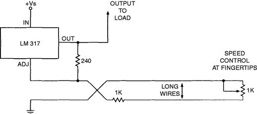
Figure 1.154 By merely swapping two wires, the ESD pulse is now sent to ground and does no harm
A similar situation occurs when you get a complaint from Boston in June, “Your op-amps don’t meet spec for bias current.” The solution is surprisingly simple: Usually a good scrub with soap and water works better than any other solvent to clean off the residual contaminants that cause leakage under humid conditions. (Fingerprints, for example…)
1.7.11 When Computers Replace Troubleshooters, Look Out
Now, let’s think—what needs troubleshooting? Circuits? Television receivers? Cars? People? Surely doctors have a lot of troubleshooting to—they listen to symptoms and try to figure out the solution. What is the natural temptation? To let a computer do all the work! After all, a computer is quite good at listening to complaints and symptoms, asking wise questions, and proposing a wise diagnosis. Such a computer system is sometimes called an Expert System—part of the general field of Artificial Intelligence. But, I am still in favor of genuine intelligence. Conversely, people who rely on Artificial Intelligence are able to solve some kinds of problems, but you can never be sure if they can accommodate every kind of Genuine Stupidity as well as Artificial Stupidity. (That is the kind that is made up especially to prove that Artificial Intelligence works just great.)
I won’t argue that the computer isn’t a natural for this job; it will probably be cost-effective, and it won’t be absent-minded. But, I am definitely nervous because if computers do all the routine work, soon there will be nobody left to do the thinking when the computer gives up and admits it is stumped. I sure hope we don’t let the computers leave the smart troubleshooting people without jobs, whether the object is circuits or people.
My concern is shared by Dr. Nicholas Lembo, the author of a study on how physicians make diagnoses, which was published in the New England Journal of Medicine. He recently told the Los Angeles Times, “With the advent of all the new technology, physicians aren’t all that much interested (in bedside medicine) because they can order a $300 to $400 test to tell them something they could have found by listening.” An editorial accompanying the study commented sadly: “The present trend…may soon leave us with a whole new generation of young physicians who have no confidence in their own ability to make worthwhile bedside diagnoses.” Troubleshooting is still an art, and it is important to encourage those artists.
1.7.12 The Computer Is Your Helper … and Friend …???
I read in the San Francisco Examiner (Ref. 1.9) about a case when SAS, the Scandinavian airline, implemented an “Expert System” for its mechanics:
“Management knew something was wrong when the quality of the work started decreasing. It found the system was so highly mechanized that mechanics never questioned its judgment. So the mechanics got involved in its redesign. They made more decisions on the shop floor and used the computer to augment those decisions, increasing productivity and cutting down on errors. ‘A computer can never take over everything,’ said one mechanic. ‘Now there are greater demands on my judgment, (my job) is more interesting.’” What can I add? Just be thoughtful. Be careful about letting the computers take over.
1.7.13 No Problems?? No Problem … Just Wait …
Now, let’s skip ahead and presume we have all the necessary tools and the right receptive attitude. What else do we need? What is the last missing ingredient? That reminds me of the little girl in Sunday School who was asked what you have to do to obtain forgiveness of sin. She shyly replied, “First you have to sin.” So, to do troubleshooting, first you have to have some trouble. But, that’s usually not a problem; just wait a few hours, and you’ll have plenty. Murphy’s Law implies that if you are not prepared for trouble, you will get a lot of it. Conversely, if you have done all your homework, you may avoid most of the possible trouble.
I’ve tried to give you some insights on the philosophy of how to troubleshoot. Don’t believe that you can get help on a given problem from only one specific person. In any particular case, you can’t predict who might provide the solution. Conversely, when your buddy is in trouble and needs help, give it a try—you could turn out to be a hero. And, even if you don’t guess correctly, when you do find out what the solution is, you’ll have added another tool to your bag of tricks.
When you have problems, try to think about the right plan to attack and nail down the problem. So, if you do your “philosophy homework,” it may make life easier and better for you. You’ll be able not only to solve problems, but maybe even to avoid problems. That sounds like a good idea to me!
1.7.14 Choosing the Right Equipment
As discussed earlier, the most important thing you need for effective troubleshooting is your wits. In addition to those, however, you’ll normally want to have some equipment. This section itemizes the equipment that is necessary for most general troubleshooting tasks; some you can buy off the shelf, and some you can build yourself.
Before you begin your troubleshooting task, you should know that the equipment you use has a direct bearing on the time and effort you must spend to get the job done. Also know that the equipment you need to do a good job depends on the kind of circuit or product you are working on. For example, a DVM may be unnecessary for troubleshooting some problems in digital logic. And, the availability and accessibility of equipment may present certain obstacles. If you only have a mediocre oscilloscope and your company can’t go out and buy or rent or borrow a fancy full-featured scope, then you will have to make do.
If you lack a piece of equipment, be aware that you are going into battle with inadequate tools; certain clues may take you much longer than necessary to spot. In many cases when you spent too much time finding one small problem, the time was wasted simply because you were foolish or were unaware of a particular troubleshooting technique; but, in other cases, the time was wasted because of the lack of a particular piece of equipment. It’s important for you to recognize this last-mentioned situation. Learning when you’re wasting time because you lack the proper equipment is part of your education as a troubleshooter.
In addition to the proper tools, you also need to have a full understanding of how both your circuit and your equipment are supposed to work. I’m sure you’ve seen engineers or technicians work for many fruitless hours on a problem and then, when they finally find the solution, say, “Oh, I didn’t know it was supposed to work that way.” You can avoid this scenario by using equipment that you are comfortable and familiar with.
The following equipment is essential for most analog-circuit troubleshooting tasks. This list can serve as a guide to both those setting up a lab and those who just want to make sure that they have everything they need—that they aren’t missing any tricks.
1. A dual-trace oscilloscope. It’s best to have one with a sensitivity of 1 or 2 mV/cm and a bandwidth of at least 100 MHz. Even when you are working with slow op-amps, a wide-bandwidth scope is important because some transistors in “slow” applications can oscillate in the range of 80 or 160 MHz, and you should be able to see these little screams. Of course, when working with fast circuits, you may need to commandeer the lab’s fastest scope to look for glitches. Sometimes a peak-to-peak automatic triggering mode is helpful and time-saving. Be sure you know how all the controls work, so you don’t waste much time with setup and false-triggering problems.
2. Two or three scope probes. They should be in good condition and have suitable hooks or points. Switchable 1 ×/10× probes are useful for looking at both large and very small signals. You should be aware that 1× probes only have a 16- or 20-MHz bandwidth, even when used with a 100-MHz scope. When you use 10× probes, be sure to adjust the capacitive compensation of the probe by using the square-wave calibrator per Figure 1.155. Failure to do so can be a terrible time-wasting source of trouble.
Ideally, you’ll want three probes at your disposal, so that you can have one for the trigger input and one for each channel. For general-purpose troubleshooting, the probes should have a long ground wire, but for high-speed waveforms you’ll need to change to a short ground wire (Figure 1.156) The shorter ground wires not only give you better frequency response and step response for your signal, but also better rejection of other noises around your circuit.
In some high-impedance circuits, even a 10× probe’s capacitance, which is typically 9 to 15 pF, may be unacceptable. For these circuits, you can buy an active probe with a lower input capacitance of 1.5 to 3 pF ($395 to $1800), or you can build your own (Figure 1.157).
When you have to work with switching regulators, you should have a couple of current probes, so you can tell what those current signals are doing. Some current probes go down to DC; others are inherently AC coupled (and are much less expensive).
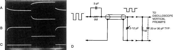
Figure 1.155 If an amplifier or a comparator is supposed to produce a square wave but the waveform looks like trace (A) or (B), how long should it take you to find the problem? No time at all! Just turn the screw that adjusts the 10 × probe’s compensation, so the probe’s response is flat at all frequencies (C). The schematic diagram of a typical 10 × oscilloscope probe is shown in (D).
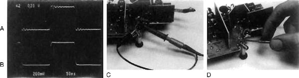
Figure 1.156 When a fast square wave is supposed to be clean and fast-settling but looks like (A), don’t repair the square-wave generator—just set aside the probe’s 6-inch ground lead (C). If you ground the probe directly at the ground point near the tip (D) (special attachments that bring the ground out conveniently are available), your waveforms will improve considerably (B).

Figure 1.157 This probe circuit’s input impedance is 1011Ω in parallel with 0.29 pF (A). Optimized primarily for its impedance characteristics and not its frequency response, the probe’s bandwidth and slew rate are 90 MHz and 300V/μs, respectively. If the lack of physical rigidity of the TO-92 packaged FET makes it too wobbly to use as a probe, a piece of 1/16-in. glass epoxy board with the copper peeled off will add rigidity with only 0.08 pF of additional capacitance. The layout of the drilled-out beam shown in the top of Figure 1.157(B) adds only 0.06 pF to the input capacitance.

Figure 1.158 Even if it’s battery-powered, a DVM is capable of Spitting out noise pulses into your delicate circuit. The RC filters shown here can help minimize this. Pick the values that work for your circuit.
3. An analog-storage oscilloscope. Such a scope can be extremely useful, especially when you are searching for an intermittent or evanescent signal. The scope can trigger off an event that may occur only rarely and can store that event and the events that follow it. Some storage scopes are balky or tricky to apply, but it’s often worth- while to expend the effort to learn how to use them. Digital-storage oscilloscopes (DSOs) let you do the same type of triggering and event storage as do the analog type, and some can display events that precede the trigger. They are sampled-data systems, however, so you must be sure to apply them correctly (Ref. 1.10). Once you learn how to use them, though, you’ll appreciate the special features they offer, such as bright CRT displays, automatic pulse-parameter measurements, and the ability to obtain plots of waveforms.
4. A digital voltmeter (DVM). Choose one with at least five digits of resolution, such as the HP3455, the HP3456, the Fluke 8810A, or the Fluke 8842A. Be sure you can lock out the autorange feature, so that the unit can achieve its highest accuracy and speed. Otherwise, you’ll be wasting time while the DVM autoranges. For many analog circuits, it’s important to have a high-impedance (>>10,000 MΩ) input that stays at high impedance up to 15 or 20V; the four DVMs mentioned above have this feature. There are many other fine DVMs that have 10 MR inputs above 2 or 3V; and, if a 10 MΩ input impedance is not a problem, they are acceptable. The most important reason to use a high-input-impedance DVM is because sometimes it’s necessary to put 33 kΩ or 100 kΩ resistors in series with the probe, right near the circuit-under-test, to prevent the DVM’s input capacitance from causing the circuit to oscillate. If you’re using a DVM with a 10 MΩ input impedance and you have a 100 kΩ resistor in series with the probe, the DVM’s measurements would lose 1% of their accuracy. Fortunately, many good DVMs have less than 500 pA of input current, which would cause less than 50 μV of error in the case of 100 kΩ source resistance. A high-resolution DVM lets you detect 100- to 200-μV deviations in an 11V signal. You can best spot many semiconductor problems by finding these minor changes. A 4-digit DVM is a relatively poor tool; however, if you are desperate. you can detect small voltage changes if you refer the DVM’s “low,” or ground, side to a stable reference, such as a 10V bus. Then, with the DVM in the IV range, you can spot small deviations in an 11V signal. This measurement is more awkward and inconvenient than a ground-referenced measurement with a higher resolution meter would be, and this method can cause other problems as well. For instance, you can end up injecting noise generated by the DVM’s A/D converter into the sensitive IO-V reference, thereby adversely affecting the performance of other circuits. In some cases, a little RC filtering may minimize this problem (see Figure 1.158) but you never can be sure how easy it will be to get the noise to an acceptable level…
5. Auxiliary meters. It may look silly to see a test setup consisting of two good DVM’s, two little 3-digit DVMs monitoring a couple of voltage supplies. A couple more 3-digit DVMs monitoring current drain, and an analog meter monitoring something else. But, if you don’t know exactly what you’re looking for and you can borrow equipment, using lots of meters is an excellent way to attack a problem—even if you do have to wait until 5:15 PM to borrow all that equipment. When is an analog volt-meter better than a DVM? Well, the analog voltmeter usually has inferior accuracy and resolution, but when you watch an ordinary analog voltmeter your eye can detect a trend or rate-of-change that may be hard to spot on a DVM, especially in the presence of noise or jitter. As an example, if you suddenly connect an ordinary analog volt-ohmmeter across a 1 μF capacitor, your eye can resolve if the capacitor’s value is 0.1 times or 10 times as large as it should be. You can’t perform this kind of test with a DVM. Another advantage of analog meters is that they are passive devices: They don’t inject noise into your circuit as digital meters can—even battery-powered ones. And they can have a lot less capacitance to ground.
6. A general-purpose function generator. While sine and square waves are popular test signals, I have often found triangular waveforms to be invaluable when searching for nonlinearities. Sometimes you need two function generators, one to sweep the operating point of the DUT, slowly, back and forth over its operating range, while you watch the response of the output to a small quick square wave—watching for oscillation or ringing or trouble.
7. Power supplies with stable outputs. They should have coarse and fine adjustment controls and adjustable current limits. Digital controls are usually not suitable; they don’t let you continuously sweep the voltage up and down while you monitor the scope and watch for trends. In cases when the power supply’s output capacitor causes problems, you may want a power supply whose output circuit, like that of an op-amp, includes no output capacitor. You can buy such a supply, or you can make it with an op-amp and a few transistors. The advantage of the supply shown in Figure 1.159 is that you can design it to slew fast when you want it to.
(For speed, use a quick LF356 rather than a slow LM741). Also, if a circuit latches and pulls its power supply down, the circuit won’t destroy itself by discharging a big capacitor.
While we are on the topic of power, another useful troubleshooting tool is a set of batteries. You can use a stack of one, two, or four 9V batteries, ni-cads, gel cells, or whatever is suitable and convenient. Batteries are useful as an alternate power supply for low-noise preamplifiers: If the preamp’s output doesn’t get quieter when the batteries are substituted for the ordinary power supply, don’t blame your circuit troubles on the power supply. You can also use these batteries to power low-noise circuits, such as those sealed in a metal box, without contaminating their signals with any external noise sources.
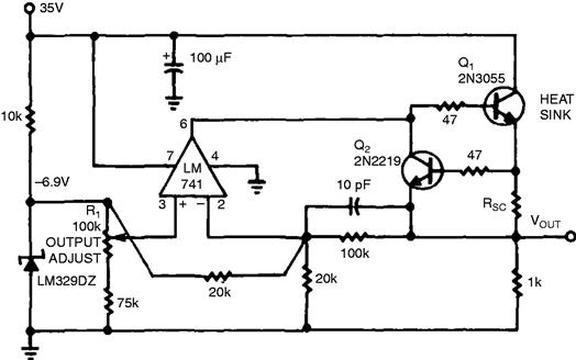
Figure 1.159 You can vary the output voltage of this DC power supply from 3 to 30V by adjusting R1. Rsc should be between 3 and 100Ω; the short-circuit current is equal to about 20 mA + 600 mV/ Rsc

Figure 1.160 This general schematic is for a commercially available RC substitution box, the VIZ Model WC-4I2A. The unit costs around $139 in 1991 dollars and has resistor and capacitor values in the range of 15Ω to 10 MΩ and 100 pF to 0.2 μF, respectively. It can be configured to be an open circuit, a series RC, resistors, capacitors, a parallel RC, or a short circuit. See text for availability.
8. A few RC substitution boxes. You can purchase the VIZ Model WC-412A, which I refer to affectionately as a “Twiddle-box” (Figure 1.160) from R & D Electronics, 1432 South Main Street, Milpitas CA 95035, (408) 262-7144. Or, inquire at VIZ, 175 Commerce Drive, Fort Washington, PA 19034, (800) 523-3696. You can set the unit in the following modes: R, C, series RC, parallel RC, open circuit, or short circuit. They are invaluable for running various “tests” that can lead to the right answer.
You may need component values beyond what the twiddle boxes offer; in our labs, we built a couple of home-brew versions (Figure 1.161). The circuit shown in Figure 1.161(A) provides variable low values of capacitance and is useful for fooling around with the damping of op-amps and other delicate circuits. You can make your own calibration labels to mark the setting of the capacitance and resistance values. The circuit shown in Figure 1.161(B) provides high capacitances of various types, for testing power supplies and damping various regulators.

Figure 1.161 RC boxes based on these schematics extend component ranges beyond those available in off-the-shelf versions. You can house the series RC circuit in (A) in a 1 × 1 × 2-inch copper-clad box. Use the smaller plastic-film-dielectric tuning capacitors or whatever is convenient, and a small I -turn pot. Build the circuit in (B) with tantalum or electrolytic (for values of 1 μF and higher) capacitors, but remember to be careful about their polarities and how you apply them. Also, you might consider using mylar capacitors for smaller values. Sometimes it’s very valuable to compare a mylar, a tantalum, and an aluminum electrolytic capacitor of the same value! Use 18-position switches to select R and C values. And, stay away from wirewound resistors; their inductance is too high.
9. An isolation transformer. If you are working on a line-operated switching regulator, this transformer helps you avoid lethal and illegal voltages on your test setup and on the body of your scope. If you have trouble obtaining an isolation transformer. you can use a pair of transformers (step-down, step-up) back-to-back (Figure 1.162). Or. If cost isn’t an issue, you can use isolated probes. These probes let you display small signals that have common-mode voltages of hundreds of volts with respect to ground, and they won’t require you to wear insulated gloves when adjusting your scope.

Figure 1.162 You can use this back-to-back transformer configuration to achieve line isolation similar to that of an isolation transformer.
10. A variable autotransformer, often called a Variac™.1 This instrument lets you change the line voltage and watch its effect on the circuit—a very useful trick. (Warning: A variable autotransformer is not normally an isolation transformer. You may need to cascade one of each, to get safe adjustable power.)
11. A curve tracer. A curve tracer can show you that two transistors may have the same saturation voltage under a given set of conditions even though the slope of one may be quite different from the slope of the other. If one of these transistors works well and the other badly, a curve tracer can help you understand why. A curve tracer can also be useful for spotting nonlinear resistances and conductances in diodes, capacitors, light bulbs, and resistors. A curve tracer can test a battery by loading it down or recharging it. It can check semiconductors for breakdown. And, when you buy the right adapters or cobble them up yourself, you can evaluate the shape of the gain, the CMRR, and the PSRR of op-amps.
12. Spare repair parts for the circuit-under-test. You should have these parts readily available, so you can swap components to make sure they still work correctly.
13. A complete supply of resistors and capacitors. You should have resistors in the range from 0.1Ω to 100 MΩ and capacitors from 10 pF to 1 μF. Also, 10,100, and 1000 μF capacitors come in handy. Just because your circuit design doesn’t include a 0.1Ω or a 100 MΩ resistor doesn’t mean that these values won’t be helpful in troubleshooting it. Similarly, you may not have a big capacitor in your circuit; but, if the circuit suddenly stops misbehaving when you put a 3800 μF capacitor across the power supply, you’ve seen a quick and dramatic demonstration that power-supply wobbles have a lot to do with the circuit’s problems. Also, several feet of plastic-insulated solid wire (telephone wire) often come in handy. A few inches of this type of twisted-pair wire makes an excellent variable capacitor, sometimes called a gimmick. Gimmicks are cheap and easy to vary by simply winding or unwinding them. Their capacitance is approximately one picofarad per inch.
14. Schematic diagrams. It’s a good idea to have several copies of the schematic of the circuit-under-test. Mark up one copy with the normal voltages, currents, and waveforms to serve as a reference point. Use the others to record notes and waveform sketches that relate to the specific circuit-under-test. You’ll also need a schematic of any homemade test circuit you plan to use. Sometimes, measurements made with your homemade test equipment may not agree with measurements made by purchased test equipment. The results from each tester may not really be “wrong”: They might differ because of some design feature, such as signal filtering. If you have all the schematics for your test equipment, you can more easily explain these incompatibilities. And, finally, the data sheets and schematics of any ICs used in your circuit will also come in handy.
15. Access to any engineering or production test equipment, if possible. Use this equipment to be sure that when you fix one part of the circuit, you aren’t adversely affecting another part. Other pieces of equipment and testers also fall under the category of specialized test equipment; their usefulness will depend on your circuit. Three examples are a short-circuit-detector circuit, an AM transistor radio, and a grid-dip meter.
A short-circuit-detector circuit. This tool comes in handy when you have to repair a lot of large PC boards: It can help you find a short circuit between the ground bus and the power or signal busses. It’s true that a sensitive DVM can also perform this function, but a short-circuit detector is much faster and more efficient. Also, this circuit turns itself off and draws no current when the probe is not connected. In the short-circuit-detector circuit shown in Figure 1.163, the LM10 op-amp amplifies the voltage drop and feeds it to the LM331 voltage-to-frequency converter, which you set up to emit its highest pitch when Vin = 0 mV. When using this circuit, use a 50- to 100-mA current-limited power supply. To calibrate the circuit, first ground the detector’s two probes and trim the OFFSET ADJUST for a high pitch. Then, move the positive test probe to Vs at A and trim the GAIN ADJUST for a low pitch. Figure 1.163 illustrates a case in which one of the five major power supply busses of the circuit-in-trouble has a solder short to ground.
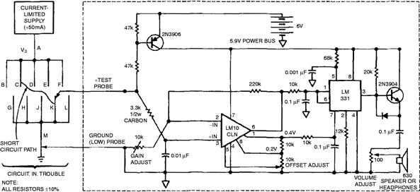
Figure 1.163 You can use this short-circuit detector to find PC board shorts. Simply slide the test probe along the various busses and listen for changes in pitch.
To find the exact location of the short, you simply slide the positive input probe along the busses. In this example, if you slide it from A toward B or D, the pitch won’t change because there is no change in voltage at these points—no current flowing along those busses. But, if you slide the probe along the path from A to C or from K to M, the pitch will change because the voltage drop is changing along those paths. It’s an easy and natural technique to learn to follow the shifting frequency signals.
An AM radio. What do you do when trouble is everywhere? A typical scenario starts out like this: You make a minor improvement on a linear circuit, and when you fire it up you notice a terrible oscillation riding on the circuit’s output. You check everything about the circuit, but the oscillation remains. In fact, the oscillation is riding on the output, the inputs, on several internal nodes. and even on ground. You turn off the DVM, the function generator, the soldering iron, and finally even the power supplies, but the oscillation is still there.
Now you start looking around the lab to see who has started a new oscillator or switching regulator that is doubling as a medium-power transmitter. Aside from yelling, “Who has a new circuit oscillating at 87 kHz?” what can you do to solve the problem? One useful tool is an ordinary AM transistor radio. As we have all learned, FM radios reject many kinds of noise, but AM radios scoop up noise at repetition rates and frequencies that would surprise you.
How can a crummy little receiver with an audio bandwidth of perhaps 5 kHz detect noise in the kilohertz and megahertz regions? Of course, the answer is that many repetitive noise-pulse trains (whose repetition rates are higher than the audible spectrum but below the AM frequency band) have harmonics that extend into the vicinity of 600 kHz, where the AM receiver is quite sensitive. This sensitivity extends to signals with amplitudes of just a few microvolts per meter.
If you are skeptical about an AM radio’s ability to detect these signals, tune its dial down to the low end, between stations. Then, hold it near a DVM or a computer or computer keyboard, and listen for the hash. Notice, too, that the ferrite stick antenna has definite directional sensitivity, so you can estimate where the noise is coming from by using either the null mode or pointing the antenna to get the strongest signal. So, the humble AM radio may be able to help you as you hike around the lab and smile pleasantly at your comrades until you find the culprit whose new switching regulator isn’t working quite right but which he neglected to turn off when he went out to get a cup of coffee.
The grid-dip meter. On other occasions, the frequency and repetition rate of the noise are so high that an AM receiver won’t be helpful in detecting the problem. What’s the tool to use then? Back in the early days of radio, engineers found that if you ran a vacuum-tube oscillator and immersed it in a field of high-power oscillations at a comparable frequency, the tube’s grid current would shift or dip when the frequencies matched. This tool became known as the “grid-dip meter.” I can’t say that I am an expert in the theory or usage of the grid-dip meter, but I do recall being impressed in the early days of monolithic ICs: A particular linear circuit was oscillating at 98 MHz, and the grid-dip meter could tickle the apparent rectified output error as I tuned the frequency dial back and forth.
That was 25 years ago, and, of course, Heathkit2 has discontinued their old Grid Dip and Tunnel Dip meters in favor of a more modern design. The new one, simply dubbed HD-1250 “Dip Meter,” uses transistors and tetrode FETs. At the bargain price of $89, every lab should have one. They’ll help you ferret out the source of nasty oscillations as high as 250 MHz. The literature that comes with the HD-1250 dip-meter kit also lists several troubleshooting tips.
When grid-dip meters first became popular, the fastest oscilloscope you could buy had a bandwidth of only a few dozen megahertz. These days, it is possible to buy a scope with a bandwidth of many hundreds of megahertz, so there are fewer occasions when you might need a grid-dip meter. Still, there are times when it is exactly the right tool. For example, you can use its oscillator to activate passive tuned circuits and detect their modes of resonance. Also, in a small company where you can’t afford to shell out the many thousands of dollars for a fast scope, the dip meter is an inexpensive alternative.
16. A few working circuits, if available. By comparing a bad unit to a good one, you can often identify problems. You can also use the good circuits to make sure that your specialized test equipment is working properly.
17. A sturdy, broad workbench. It should be equipped with a ground plane of metal that you can easily connect to the power ground. The purpose of this ground plane is to keep RF. 60-Hz, and all other noise from coupling into the circuit. Place insulating cardboard between the bench and the circuit-under-test. so that nothing tends to short to ground. Another way to prevent noise from interfering with the circuit is to use a broad sheet of single-sided copper-clad board. Placed copper-side down and with a ground wire soldered to the copper. it provides an alternate ground plane. To prevent electrostatic-discharge (ESD) damage to CMOS circuits, you’ll need a wrist strap to ground your body through 1 MΩ.
18. Safety equipment. When working on medium- or high-power circuits that might explode with considerable power in the case of a fault condition, you should be wearing safety goggles or glasses with safety lenses. Keep a fire extinguisher nearby, too.
19. A suitable hot soldering iron. If you have to solder or unsolder heavy busses from broad PC-board traces, use a big-enough iron or gun. For small and delicate traces around ICs, a small tip is essential. And, be sure that the iron is hot enough. An easy way to delaminate a trace or pad, whether you want to or not, is to heat it for too long a time, which might happen if your iron weren’t big enough or hot enough. (The old Heathkit warnings not to use a hot iron became obsolete along with the germanium transistor.) In some cases, a grounded soldering iron is required: in others, a portable (ungrounded or rechargeable) soldering iron is ideal. Make sure you know whether your iron is grounded or floating.
20. Tools for removing solder, such as solder wick or a solder sucker. You should be comfortable with whatever tools you are using; a well-practiced technique is sometimes critical for getting good results. If you are working on static-sensitive components, an antistatic solder-sucker is less likely to generate high voltages due to internal friction than is an ordinary solder-sucker. I have been cautioned that a large solder-sucker may cause problems when working on narrow PC traces: in that case, solder wick may be the better choice.
21. Hand tools. Among the tools you’ll need are sharp diagonal nippers, suitable pliers, Screwdrivers, large cutters, wrenches, wire strippers, and a jack knife or Exacto™ knife.
22. Signal leads, connectors, cables, BNC adapters, wires, clip leads, ball hooks, and alligator clips—as needed. Scrimping and chintzing in this area can waste lots of time: shaky leads can fall off or short out.
23. Freeze mist and a hair dryer. The freeze mist available in aerosol cans lets you quickly cool individual components. A hair dryer lets you warm up a whole circuit. You’ll want to know the dryer’s output air temperature because that’s the temperature to which you’ll be heating the components.
NOTE: Ideally we should not use cooling sprays based on chlorofluorocarbons (CFCs), which are detrimental to the environment. I have a few cans that some people would say I shouldn’t use. But what else should I do—send the can to the dump? Then it will soon enter the atmosphere, without doing anybody any good. I will continue to use up any sprays with CFC-based propellants that I already have, but when it is time to buy more, I’ll buy environmentally safe ones.
24. A magnifying glass or hand lens. These devices are useful for inspecting boards, wires, and components for cracks, flaws, hairline solder shorts, and cold-soldered joints.
25. An incandescent lamp or flashlight. You should be able to see clearly what you are doing, and bright lights also help you to inspect boards and components.
26. A thermocouple-based thermometer. If your thermometer is floating and battery powered, you can connect the thermocouple to any point in the circuit and measure the correct temperature with virtually no electrical or thermal effect on the circuit. Figure 1.164 shows a thermocouple amplifier with designed-in cold-junction compensation.
Some people have suggested that an LM35 temperature-sensor IC (Figure 1.165) is a simple way to measure temperature, and so it is. But, if you touch or solder an LM35 in its TO-46 package to a resistor or a device in a TO-5 or TO-3 case, the LM35 will increase the thermal mass and its leads will conduct heat away from the device whose temperature you are trying to measure. Thus, your measurements will be less accurate than if you had used a tiny thermocouple with small wires.
27. Little filters in neat metal boxes, to facilitate getting a good signal-to-noise ratio when you want to feed a signal to a scope. They should be set up with switch-selectable cut-off frequencies, and neat connectors. If in your business you need sharp roll-offs, well, you can roll your own. Maybe even with op-amps and batteries. You figure out what you need. Usually I just need a couple simple Rs and Cs, with an alligator clip to select the right ones.
28. Line adapters—those 3-wire-to-2-wire adapters for your 3-prong power cords. You need several of them. You only need them because too many scopes and function generators have their ground tied to the line-cord’s neutral. You need some of these to avoid ground-loops. You also need a few spares because your buddies will steal yours. For that matter, keep a few spare cube taps. When they rewired our benches a few years ago, the electricians tried to give us five outlets per bench. I stamped my feet and insisted on ten per bench, and that’s just barely enough, most of the time.

Figure 1.164 This thermocouple amplifier has inherent cold-junction compensation because of the two halves of Q1 which run at a 1 6:1 current ratio. Their VBEs are mismatched by 1 2 mV + 40.8 μv/°C. This mismatch exactly cancels out the 40.8 μv/°C of the cold junction. For best results, you should use four 100 kΩ resistors in series for R1 and two 100 kΩ resistors in series with two 100 kΩ resistors in parallel for R2—all resistors of the same type, from the same manufacturer. Q2 and its surrounding components implement a correction for very cold temperatures and are not necessary for thermocouple temperatures above 0°C. Credit to Mineo Yamatake for his elegant circuit design.
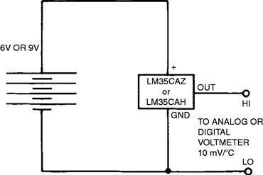
Figure 1.165 The LM35CAZ is a good, simple, convenient general-purpose temperature sensor. But beware of using it to measure the temperature of very small objects or in the case of extreme temperature gradients; it would then give you less accurate readings than a tiny thermocouple with small wires.
You’ve come to the end of my list of essential equipment for ordinary analog circuit troubleshooting. Depending on your circuit, you may not need all these items; and, of course, the list did not include a multitude of other equipment that you may find useful. Logic analyzers, impedance analyzers, spectrum analyzers, programmable current pumps, capacitance meters and testers, and pulse generators can all ease various troubleshooting tasks.
References
[1.1] Frederiksen Thomas M. Intuitive IC Op Amps National Semiconductor Corp. 1984.
[1.2] Reliance Motion Control, Inc., “Pink Motor Book” DC Motors Speed Controls Servo Systems, The Electro-Craft Engineering Handbook.
[1.3] Van Doren, Dr. Tom, Grounding and Shielding of Electronic Systems, University Missouri Rolla, Van Doren Company, Rt. 6, Box 319, Rolla, MO 65401.
[1.4] Weyrick, Robert C., Yellow Control Theory: Fundamentals of Automatic Control, McGraw Hill, ISBN 0-07-069493-1. Good read, helped me understand control theory.
[1.5] Dostal Jiri. Operational Amplifiers The Netherlands: Elsevier Scientific; 1981; also, Elsevier Scientific, Inc., 655 Avenue of the Americas, NY, NY 10010. (212) 989-5800.
[1.6] Smith John I. Modern Operational Circuit Design New York, NY: John Wiley & Sons; 1971.
[1.7] Data Converter Handbook. P.O. Box 9106, Norwood MA 02062: Analog Devices Corp., 1984.
[1.8] Bulleid HAV. In: Master Builders of Steam. London, UK: Ian Allan Ltd., 1963;146–147.
[1.9] Caruso Denise. “Technology designed by its users,” The San Francisco. Examiner Sunday, March 18, 1990; E-15.
[1.10] Collins Jack, David White. Time-domain analysis of aliasing helps to alleviate DSO errors. EDN September 15, 1988;207.