Chapter 12. Risk Analysis and Assessment

Search in book...
Toggle Font Controls
Create new playlist

Name your new playlist

Playlist description (optional)
Sign In

Email address

Password

Forgot Password?

or

Continue with Facebook

Continue with Google
Sign Up

Full Name

Email address

Confirm Email Address

Password

or

Continue with Facebook

Continue with Google

Chapter 12. Risk Analysis and Assessment

The learning objectives for this chapter are to learn and understand concepts that are commonly used by industry to conduct risk analysis and assessment. This includes:

Probability theory.
Event tree and fault tree analysis.
Risk analysis and assessment methods, including quantitative risk analysis (QRA), layer of protection analysis (LOPA) and bow-tie methods.
Societal and individual risk, and how these are quantified.
Risk tolerance criteria.

Risk is a measure of human injury, environmental damage, or economic loss in terms of both the likelihood and the magnitude of the loss. Risk analysis determines all the incident scenarios of a plant having a consequence of concern and their corresponding risks, and then sums the risks to establish the total risk for the plant. Risk assessment considers the risks and the tolerable risk criteria to make decisions regarding risk reduction.

The first part of this chapter explains how to determine the frequency of incident scenarios and how this information is used in event and fault trees. The last part explains how the frequencies are used in QRA, LOPA, qualitative, and bow-tie methods.

12-1 Review of Probability Theory

Equipment failures or faults in a process occur as a result of complex interactions of the individual components. The overall probability of a failure in a process depends on the nature of these interactions. In this section, we define the various types of interactions and describe how to compute failure probabilities.

Data are collected on the failure rate of a particular hardware component. With adequate data, it can be shown that, on average, the component fails after a certain period of time. This is called the average failure rate and is represented by μ with units of faults/time. The probability that the component will not fail during the time interval (0, t) is given by a Poisson distribution:¹

$\begin{matrix} R (t) = e^{- μ t} & (12 - 1) \end{matrix}$ $\begin{matrix} R (t) = e^{- μ t} & (12 - 1) \end{matrix}$

¹B. Roffel and J. E. Rijnsdorp. Process Dynamics, Control, and Protection (Ann Arbor, MI: Ann Arbor Science, 1982), p. 381.

where R is the reliability. Equation 12-1 assumes a constant failure rate μ. As t → ∞, the reliability goes to 0. The speed at which this occurs depends on the value of the failure rate μ. The higher the failure rate, the more rapidly the reliability decreases. Other, more complex distributions are also available, but this simple exponential distribution is most commonly used because it requires only a single parameter, μ.

The complement of the reliability is called the failure probability (or sometimes the unreliability), P, and it is given by

$\begin{matrix} P (t) = 1 - R (t) = 1 - e^{- μ t} & (12 - 2) \end{matrix}$ $\begin{matrix} P (t) = 1 - R (t) = 1 - e^{- μ t} & (12 - 2) \end{matrix}$

The failure density function is defined as the derivative of the failure probability:

$\begin{matrix} f (t) = \frac{d P (t)}{d t} = μ e^{- μ t} & (12 - 3) \end{matrix}$ $\begin{matrix} f (t) = \frac{d P (t)}{d t} = μ e^{- μ t} & (12 - 3) \end{matrix}$

The area under the complete failure density function is 1.

The failure density function is used to determine the probability P of at least one failure in the time period t₀ to t₁:

$\begin{matrix} P (t_{o} \to t_{1}) = \int_{t_{0}}^{t_{1}} f (t) d t = μ \int_{t_{0}}^{t_{1}} e^{- μ t} d t = e^{- μ t_{0}} - e^{- μ t_{1}} & (12 - 4) \end{matrix}$ $\begin{matrix} P (t_{o} \to t_{1}) = \int_{t_{0}}^{t_{1}} f (t) d t = μ \int_{t_{0}}^{t_{1}} e^{- μ t} d t = e^{- μ t_{0}} - e^{- μ t_{1}} & (12 - 4) \end{matrix}$

The integral represents the fraction of the total area under the failure density function between time t₀ and t₁.

The time interval between two failures of the component is called the mean time between failures (MTBF) and is given by the first moment of the failure density function:

$\begin{matrix} E (t) = M T B F = \int_{0}^{\infty} t f (t) d t = \frac{1}{μ} & (12 - 5) \end{matrix}$ $\begin{matrix} E (t) = M T B F = \int_{0}^{\infty} t f (t) d t = \frac{1}{μ} & (12 - 5) \end{matrix}$

Typical plots of the functions μ, f, P, and R are shown in Figure 12-1.

A figure shows four plots denoting the functions mu, f, P, and R against t. — **Figure 12-1** Typical plots of (a) the failure rate μ, (b) the failure density f (t), (c) the failure probability P(t), and (d) the reliability R(t).

The plots of Failure Rate, Failure Density, Failure Probability, and Reliability are depicted as follows. Failure Rate: it is drawn for mu against t. mu is indicated to be a constant for all values of t. Failure Density: it is drawn for f of t against t. A concave up decreasing curve is drawn and the region below the curve is shaded and labeled, "Area equals 1." Failure Probability: it is drawn for P of t against t. An increasing curve, concave down is drawn, for values of P of t from 0 to 1. The function of the curve is integral over the limits 0 to t of f of t, with respect to t. Reliability: it is drawn for R of t against t. An decreasing curve, concave up is drawn, for values of R of t from 0 to 1. The function of the curve is 1 minus, lowercase p of t.

Equations 12-1 through 12-5 are valid only for a constant failure rate μ. Many components exhibit a typical bathtub failure rate, shown in Figure 12-2. In this pattern, the failure rate is highest when the component is new (infant mortality) and when it is old (old age). Between these two periods (denoted by the lines in Figure 12-2), the failure rate is reasonably constant and Equations 12-1 through 12-5 are valid.

A typical bathtub failure rate plot based on the age factor of the component is shown. — **Figure 12-2** A typical bathtub failure rate curve for process hardware. The failure rate is approximately constant over the midlife of the component.

The plot is drawn for Failure Rate mu (faults per time) against Time. A u-shaped curve is drawn, which is almost flat in the middle. The middle region which is almost flat is labeled, "Period of Approximately Constant mu." The region to the left of the period of constant which is decreasing is the period of "Infant Mortality." The region to the right of the period of constant which is increasing is the "Old Age." This infers that, the failure rate is highest at the beginning, continues to decrease rapidly as time increases and is a constant for the mid-values of time, and again continues to increase rapidly for the rest of the values of time.

Interactions between Process Units

Incidents in chemical plants are usually the result of a complicated interaction of a number of process components. The overall process failure probability is computed from the individual component probabilities.

Process components interact in two different fashions. In some cases, a process failure requires the simultaneous failure of a number of components in parallel. This parallel structure is represented by the logical AND function. This means that the failure probabilities for the individual components must be multiplied:

$\begin{matrix} P = \prod_{i = 1}^{n} P_{i} & (12 - 6) \end{matrix}$ $\begin{matrix} P = \prod_{i = 1}^{n} P_{i} & (12 - 6) \end{matrix}$

where

n is the total number of components and

P_i is the failure probability of each component.

This rule is easily memorized because for parallel components the probabilities are multiplied.

The total reliability for parallel units is given by

$\begin{matrix} R = 1 - \prod_{i = 1}^{n} (1 - R_{i}) & (12 - 7) \end{matrix}$ $\begin{matrix} R = 1 - \prod_{i = 1}^{n} (1 - R_{i}) & (12 - 7) \end{matrix}$

where R_i is the reliability of an individual process component.

Process components also interact in series. This means that a failure of any single component in the series of components will result in failure of the process. The logical OR function represents this case. For series components, the overall process reliability is found by multiplying the reliabilities for the individual components:

$\begin{matrix} R = \prod_{i = 1}^{n} R_{i} & (12 - 8) \end{matrix}$ $\begin{matrix} R = \prod_{i = 1}^{n} R_{i} & (12 - 8) \end{matrix}$

The overall failure probability is computed from

$\begin{matrix} P = 1 - \prod_{i = 1}^{n} (1 - P_{i}) & (12 - 9) \end{matrix}$ $\begin{matrix} P = 1 - \prod_{i = 1}^{n} (1 - P_{i}) & (12 - 9) \end{matrix}$

For a system composed of two components A and B, Equation 12-9 is expanded to

$\begin{matrix} P (A or B) = P (A) + P (B) - P (A) P (B) & (12 - 10) \end{matrix}$ $\begin{matrix} P (A or B) = P (A) + P (B) - P (A) P (B) & (12 - 10) \end{matrix}$

The cross-product term P(A)P(B) compensates for counting the overlapping cases twice. Consider the example of tossing a single die and determining the probability that the number of points is even or divisible by 3. In this case,

$P (even o r divisible by 3) = P (even) + P (divisible by 3) - P (even a n d divisible by 3) .$ $P (even o r divisible by 3) = P (even) + P (divisible by 3) - P (even a n d divisible by 3) .$

The last term subtracts the cases in which both conditions are satisfied.

If the failure probabilities are small (a common situation), the term P(A)P(B) is negligible, and Equation 12-10 reduces to

$\begin{matrix} P (A or B) = P (A) + P (B) & (12 - 11) \end{matrix}$ $\begin{matrix} P (A or B) = P (A) + P (B) & (12 - 11) \end{matrix}$

This result is generalized for any number of components. For this special case, Equation 12-9 reduces to

$\begin{matrix} P = \sum_{i = 1}^{n} P_{i} & (12 - 12) \end{matrix}$ $\begin{matrix} P = \sum_{i = 1}^{n} P_{i} & (12 - 12) \end{matrix}$

Failure rate data for a number of typical process components are provided in Table 12-1. These are average values determined at a typical chemical process facility. Actual values would depend on the manufacturer, the materials of construction, the design, the environment, and other factors. The assumptions in this analysis are that the failures are independent, hard, and not intermittent, and that the failure of one device does not stress adjacent devices to the point that the failure probability is increased.

Table 12-1 Failure Rate Data for Various Selected Process Components

Instrument	Faults/Year
Controller	0.29
Control valve	0.60
Flow measurement (fluids)	1.14
Flow measurement (solids)	3.75
Flow switch	1.12
Gas–liquid chromatograph	30.6
Hand valve	0.13
Indicator lamp	0.044
Level measurement (liquids)	1.70
Level measurement (solids)	6.86
Oxygen analyzer	5.65
pH meter	5.88
Pressure measurement	1.41
Pressure relief valve	0.022
Pressure switch	0.14
Solenoid valve	0.42
Stepper motor	0.044
Strip chart recorder	0.22
Thermocouple temperature measurement	0.52
Thermometer temperature measurement	0.027
Valve positioner	0.44

Source: Selected from Frank P. Lees. Loss Prevention in the Process Industries (London, UK: Butterworths, 1986), p. 343.

A summary of computations for parallel and series process components is shown in Figure 12-3.

A figure summarizes the different computation combinations for process components. — **Figure 12-3** Computations for various types of component linkages.

A figure shows the Series and Parallel link of components to compute Failure Probability, Reliability, and Failure Rate. They are as follows. Series link of components: Failure Probability: An OR gate with two inputs P1 and P2 and an output P is shown. P equals 1 minus, the product of 1 minus P1 and 1 minus P2. Hence, P equals 1 minus the Product of (1 minus P i), for i equals 1 to n. Reliability: An OR gate with two inputs R1 and R2 and an output R is shown. R equals R1 times R2. Hence, R equals the Product of Ri, where i equals 1 to n. Failure Rate: An OR gate with two inputs mu 1 and mu 2 and an output mu is given. mu equals mu 1 plus mu 2. Hence, mu equals the summation of mu i, where i equals 1 to n. The summarized result of Series link of component reads, "the failure of either component adds to the total system failure." Parallel link of components: Failure Probability: An AND gate with two inputs P1 and P2 and an output P is given. P equals P1 times P2. Hence, P equals the product of P i, where i equals 1 to n. Reliability: An AND gate with two inputs R1 and R2 and an output R is given. R equals 1 minus, the product of 1 minus R1 and 1 minus R2. Hence, R equals 1 minus, the product of 1 minus R i, where i equals 1 to n. Reliability: mu equals negative natural log of R over t. The summarized result of Parallel link of components reads, "the failure of the system requires the failure of both components. Note that there is no convenient way to combine the failure rate."

Example 12-1

The flow of water to a chemical reactor cooling coil is controlled by the system shown in Figure 12-4. The flow is measured by a differential pressure (DP) flow meter, the controller is designed to control the flow, and the control valve manipulates the flow of coolant. Determine the overall failure rate, the unreliability, the reliability, and the MTBF for this system. Assume a 1-year period of operation.

A figure demonstrates the setup of a flow control system. — **Figure 12-4** Flow control system. The components of the control system are linked in series.

The flow control system is depicted. The system is constituted of a Pump, a Flow Meter, a Control Valve, and a Controller. The flow of water enters the Pump, which is connected to a Flow Meter. The Flow Meter is in turn connected to a Control Valve, and the water stream passes out through the control valve. The Flow Meter and the Control Valve are connected to an F I C Controller.

Solution

These process components are related in series. Thus, if any one of the components fails, the entire system fails. The reliability and failure probability are computed for each component using Equations 12-1 and 12-2. The results are shown in the following table. The failure rates are from Table 12-1.

Component	Failure rate μ (faults/yr)	Reliability (R = e^−μt)	Failure probability (P = 1 − R)
Control valve	0.60	0.55	0.45
Controller	0.29	0.75	0.25
DP cell	1.41	0.24	0.76

The overall reliability for components in series is computed using Equation 12-8. The result is

$R = Π_{i = 1}^{3} R_{i} = (0.55) (0.75) (0.24) = 0.10$ $R = Π_{i = 1}^{3} R_{i} = (0.55) (0.75) (0.24) = 0.10$

The failure probability is computed from Equation 12-2:

$P = 1 - R = 1 - 0.10 = 0.90 /yr$ $P = 1 - R = 1 - 0.10 = 0.90 /yr$

The overall failure rate is computed using the definition of the reliability (Equation 12-1):

$\begin{matrix} R & = 0.10 = e^{- μ} \\ μ & = - \ln (0.10) = 2.3 failures/yr \end{matrix}$ $\begin{matrix} R & = 0.10 = e^{- μ} \\ μ & = - \ln (0.10) = 2.3 failures/yr \end{matrix}$

The MTBF is computed using Equation 12-5:

$MTBF = \frac{1}{μ} = 0.43 yr$ $MTBF = \frac{1}{μ} = 0.43 yr$

This system is expected to fail, on average, once every 0.43 yr.

Example 12-2

A diagram of the safety systems for a chemical reactor is shown in Figure 12-5. This reactor contains a high-pressure alarm to alert the operator in the event of dangerous reactor pressures. It consists of a pressure switch on the reactor connected to an alarm light indicator. For additional safety, an automatic high-pressure reactor shutdown system is installed. This system is activated at a pressure somewhat higher than the alarm system and consists of a pressure controller connected to a solenoid valve in the reactor feed line. The automatic system stops the flow of reactant in the event of high pressure. Compute the overall failure rate, the failure probability, the reliability, and the MTBF for a high-pressure condition. Assume a 1-year period of operation. Also, develop an expression for the overall failure probability based on the component failure probabilities.

An illustration of the safety systems setup of a chemical reactor is shown. — **Figure 12-5** A chemical reactor with an alarm and an inlet feed solenoid valve. The alarm and feed shutdown systems are linked in parallel.

A figure shows a chemical reactor with an alarm. The input feed to the Reactor is fed to the Reactor through a Solenoid Valve, which is connected to a Pressure Indicating Controller. The PIC is also connected to the Reactor. Further, on the other end, the Reactor is connected to a P I 'A' Pressure Switch, which is indicated to alarm at P greater than P subscript A.

Solution

Failure rate data are available from Table 12-1. The reliability and failure probabilities of each component are computed using Equations 12-1 and 12-2:

Component	Failure rate μ (faults/yr)	Reliability (R = e^−μt)	Failure probability (P = 1 – R)
1. Pressure switch	0.14	0.87	0.13
2. Alarm indicator	0.044	0.96	0.04
3. Pressure controller	0.14	0.87	0.13
4. Solenoid valve	0.42	0.66	0.34

A dangerous high-pressure reactor situation occurs only when both the alarm system and the shutdown system fail. These two components are in parallel. For the alarm system, the components are in series. Thus, from Equation 12-8:

$\begin{matrix} R & = \prod_{i = 1}^{2} R_{i} = (0.87) (0.96) = 0.835 \\ P & = 1 - R = 1 - 0.835 = 0.165 \\ μ & = - \ln R = - \ln (0.835) = 0.180 faults/yr \\ MTBF & = \frac{1}{μ} = 5.56 yr \end{matrix}$ $\begin{matrix} R & = \prod_{i = 1}^{2} R_{i} = (0.87) (0.96) = 0.835 \\ P & = 1 - R = 1 - 0.835 = 0.165 \\ μ & = - \ln R = - \ln (0.835) = 0.180 faults/yr \\ MTBF & = \frac{1}{μ} = 5.56 yr \end{matrix}$

For the shutdown system, the components are also in series. From Equation 12-8 and 12-5:

$\begin{matrix} R & = \prod_{i = 1}^{2} R_{i} = (0.87) (0.66) = 0.574 \\ P & = 1 - R = 1 - 0.574 = 0.426 \\ μ & = - \ln R = - \ln (0.574) = 0.555 faults/yr \\ MTBF & = \frac{1}{μ} = 1.8 yr \end{matrix}$ $\begin{matrix} R & = \prod_{i = 1}^{2} R_{i} = (0.87) (0.66) = 0.574 \\ P & = 1 - R = 1 - 0.574 = 0.426 \\ μ & = - \ln R = - \ln (0.574) = 0.555 faults/yr \\ MTBF & = \frac{1}{μ} = 1.8 yr \end{matrix}$

The two systems are combined using Equation 12-6:

$\begin{matrix} P & = \prod_{i = 1}^{2} P_{i} = (0.165) (0.426) = 0.070 \\ R & = 1 - P = 0.930 \\ μ & = - \ln R = - \ln (0.930) = 0.073 faults/yr \\ MTBF & = \frac{1}{μ} = 13.7 yr \end{matrix}$ $\begin{matrix} P & = \prod_{i = 1}^{2} P_{i} = (0.165) (0.426) = 0.070 \\ R & = 1 - P = 0.930 \\ μ & = - \ln R = - \ln (0.930) = 0.073 faults/yr \\ MTBF & = \frac{1}{μ} = 13.7 yr \end{matrix}$

For the alarm system alone, a failure is expected once every 5.6 yr. Similarly, for a reactor with a high-pressure shutdown system alone, a failure is expected once every 1.80 yr. However, with both systems in parallel, the MTBF is significantly improved and a combined failure is expected every 13.7 yr.

The overall failure probability is given by Equation 12-6:

$P = P (A) P (S)$ $P = P (A) P (S)$

where P(A) is the failure probability of the alarm system and P(S) is the failure probability of the emergency shutdown system. An alternative procedure is to use Equation 12-9 directly. For the alarm system,

$P (A) = P_{1} + P_{2} - P_{1} P_{2}$ $P (A) = P_{1} + P_{2} - P_{1} P_{2}$

For the shutdown system,

$P (S) = P_{3} + P_{4} - P_{3} P_{4}$ $P (S) = P_{3} + P_{4} - P_{3} P_{4}$

The overall failure probability is then

$P = P (A) P (S) = (P_{1} + P_{2} - P_{1} P_{2}) (P_{3} + P_{4} - P_{3} P_{4})$ $P = P (A) P (S) = (P_{1} + P_{2} - P_{1} P_{2}) (P_{3} + P_{4} - P_{3} P_{4})$

Substituting the numbers provided in the example, we obtain

$\begin{matrix} \begin{matrix} P \end{matrix} & = [0.13 + 0.04 - (0.13) (0.04)] [0.34 + 0.13 - (0.34) (0.13)] \\ = (0.165) (0.426) = 0.070 \end{matrix}$ $\begin{matrix} \begin{matrix} P \end{matrix} & = [0.13 + 0.04 - (0.13) (0.04)] [0.34 + 0.13 - (0.34) (0.13)] \\ = (0.165) (0.426) = 0.070 \end{matrix}$

This is the same answer as before.

If the products P₁P₂ and P₃P₄ are assumed to be small, then

$P (A) = P_{1} + P_{2}$ $P (A) = P_{1} + P_{2}$

and

$\begin{matrix} P & = P (A) P (S) = (P_{1} + P_{2}) (P_{3} + P_{4}) \\ = 0.080 \end{matrix}$ $\begin{matrix} P & = P (A) P (S) = (P_{1} + P_{2}) (P_{3} + P_{4}) \\ = 0.080 \end{matrix}$

The difference between this answer and the answer obtained previously is 14.3%. The component probabilities are not small enough in this example to assume that the cross-products are negligible.

Revealed and Unrevealed Failures

Example 12-2 assumes that all failures in either the alarm or the shutdown system are immediately obvious to the operator and are repaired in a negligible amount of time. Emergency alarms and shutdown systems are used only when a dangerous situation occurs. It is possible for the equipment to fail without the operator being aware of the situation—an event called an unrevealed failure. Without regular and reliable equipment testing, alarm and emergency systems can fail without notice. Failures that are immediately obvious are called revealed failures.

As an example, consider that a flat tire on a car is immediately obvious to the driver. In contrast, the spare tire in the trunk might also be flat without the driver being aware of the problem until the spare is needed.

Figure 12-6 shows the nomenclature for revealed failures. The time that the component is operational is called the period of operation and is denoted by τ_o. After a failure occurs, a period of time, called the period of inactivity or downtime (τ_r), is required to repair the component. The MTBF is the sum of the period of operation and the downtime.

A diagram shows the relationship between Component Status and Time. — **Figure 12-6** Component cycles for revealed failures. A failure requires a period of time for repair.

A graph depicts the component cycles for revealed failures. Component Status is plotted against Time. Two states are listed out as Component statuses, Operation and Failed. The component cycle is outlined as a square wave form, wavering between the two states. The waveform starts with the Failed status and changes into Operational when the Component is Repaired. Again, the status changes to Failed when the Component Fails, changing back to Operational when the Component is repaired. The time between a "Component Repaired" and the subsequent "Component Failure" is marked tau subscript o. The time between a "Component Failure" and the subsequent "Component Repaired" is marked tau subscript t. The time between two successive Component Repaired is marked MTBF.

For revealed failures, the period of inactivity or downtime for a particular component is computed by averaging the inactive period for a number of failures:

$\begin{matrix} τ_{r} ≅ \frac{1}{n} \sum_{i = 1}^{n} τ_{r_{i}} & (12 - 13) \end{matrix}$ $\begin{matrix} τ_{r} ≅ \frac{1}{n} \sum_{i = 1}^{n} τ_{r_{i}} & (12 - 13) \end{matrix}$

where

n is the number of times the failure or inactivity occurred and

τ_{r_i} is the period for repair for a particular failure.

Similarly, the time before failure or period of operation is given by

$\begin{matrix} τ_{0} ≅ \frac{1}{n} \sum_{i = 1}^{n} τ_{o_{i}} & (12 - 14) \end{matrix}$ $\begin{matrix} τ_{0} ≅ \frac{1}{n} \sum_{i = 1}^{n} τ_{o_{i}} & (12 - 14) \end{matrix}$

where τ_oi is the period of operation between a particular set of failures.

The MTBF is the sum of the period of operation and the repair period:

$\begin{matrix} M T B F = \frac{1}{μ} = τ_{r} + τ_{o} & (12 - 15) \end{matrix}$ $\begin{matrix} M T B F = \frac{1}{μ} = τ_{r} + τ_{o} & (12 - 15) \end{matrix}$

It is convenient to define the availability and the unavailability. The availability A is simply the probability that the component or process is found functioning. The unavailability U is the probability that the component or process is found not functioning. It is obvious that

$\begin{matrix} A + U = 1 & (12 - 16) \end{matrix}$ $\begin{matrix} A + U = 1 & (12 - 16) \end{matrix}$

The quantity τ_o represents the period that the process is in operation, and τ_r + τ_o represents the total time. By definition, it follows that the availability is given by

$\begin{matrix} Α = \frac{τ_{o}}{τ_{r} + τ_{o}} & (12 - 17) \end{matrix}$ $\begin{matrix} Α = \frac{τ_{o}}{τ_{r} + τ_{o}} & (12 - 17) \end{matrix}$

Similarly, the unavailability is

$\begin{matrix} U = \frac{τ_{r}}{τ_{r} + τ_{o}} . & (12 - 18) \end{matrix}$ $\begin{matrix} U = \frac{τ_{r}}{τ_{r} + τ_{o}} . & (12 - 18) \end{matrix}$

By combining Equations 12-17 and 12-18 with the result of Equation 12-15, we can write the equations for the availability and unavailability for revealed failures:

$\begin{matrix} \begin{matrix} U = μ τ_{r} \\ A = μ τ_{o} \end{matrix} & (12 - 19) \end{matrix}$ $\begin{matrix} \begin{matrix} U = μ τ_{r} \\ A = μ τ_{o} \end{matrix} & (12 - 19) \end{matrix}$

For unrevealed failures, the failure becomes obvious only after regular inspection. This situation is depicted in Figure 12-7. If τ_u is the average period of unavailability during the inspection interval and if τ_i is the inspection interval, then

$\begin{matrix} U = \frac{τ_{u}}{τ_{i}} & (12 - 20) \end{matrix}$ $\begin{matrix} U = \frac{τ_{u}}{τ_{i}} & (12 - 20) \end{matrix}$

The average period of unavailability is computed from the failure probability:

$\begin{matrix} τ_{u} = \int_{0}^{τ_{i}} P (t) d t & (12 - 21) \end{matrix}$ $\begin{matrix} τ_{u} = \int_{0}^{τ_{i}} P (t) d t & (12 - 21) \end{matrix}$

Combining with Equation 12-20, we obtain

$\begin{matrix} U = \frac{1}{τ_{i}} \int_{0}^{τ_{i}} P (t) d t & (12 - 22) \end{matrix}$ $\begin{matrix} U = \frac{1}{τ_{i}} \int_{0}^{τ_{i}} P (t) d t & (12 - 22) \end{matrix}$

The failure probability P(t) is given by Equation 12-2. This is substituted into Equation 12-22 and integrated. The result is

$\begin{matrix} U = 1 - \frac{1}{μ τ_{i}} (1 - e^{- μ τ_{i}}) & (12 - 23) \end{matrix}$ $\begin{matrix} U = 1 - \frac{1}{μ τ_{i}} (1 - e^{- μ τ_{i}}) & (12 - 23) \end{matrix}$

An expression for the availability is

$\begin{matrix} A = \frac{1}{μ τ_{i}} (1 - e^{- μ τ_{i}}) & (12 - 24) \end{matrix}$ $\begin{matrix} A = \frac{1}{μ τ_{i}} (1 - e^{- μ τ_{i}}) & (12 - 24) \end{matrix}$

If the term uτ_i ≪ 1, then the failure probability is approximated by

$\begin{matrix} P (t) \approx μ t & (12 - 25) \end{matrix}$ $\begin{matrix} P (t) \approx μ t & (12 - 25) \end{matrix}$

and Equation 12-22 is integrated to give, for unrevealed failures,

$\begin{matrix} \begin{matrix} \begin{matrix} \begin{matrix} U = \frac{1}{2} μ τ_{i} \end{matrix} \end{matrix} \end{matrix} & (12 - 26) \end{matrix}$ $\begin{matrix} \begin{matrix} \begin{matrix} \begin{matrix} U = \frac{1}{2} μ τ_{i} \end{matrix} \end{matrix} \end{matrix} & (12 - 26) \end{matrix}$

This is a useful and convenient result. It demonstrates that, on average, for unrevealed failures the process or component is unavailable during a period equal to half the inspection interval. A decrease in the inspection interval is shown to increase the availability of an unrevealed failure.

Equations 12-20 through 12-26 assume a negligible repair time. This is usually a valid assumption because online process equipment is generally repaired within hours, whereas the inspection intervals are usually monthly.

Example 12-3

Compute the availability and the unavailability for both the alarm and the shutdown systems of Example 12-2. Assume that a maintenance inspection occurs once every month and that the repair time is negligible.

Solution

Both systems demonstrate unrevealed failures. For the alarm system, the failure rate is μ = 0.18 faults/yr. The inspection period is 1/12 = 0.083 yr. The unavailability is from Equation 12-26:

$\begin{matrix} \begin{matrix} U \end{matrix} & = \frac{1}{2} μ τ_{i} = (\frac{1}{2}) (0.18 faults/yr) (0.083 yr) = 0.0075 \\ A & = 1 - U = 0.992 \end{matrix}$ $\begin{matrix} \begin{matrix} U \end{matrix} & = \frac{1}{2} μ τ_{i} = (\frac{1}{2}) (0.18 faults/yr) (0.083 yr) = 0.0075 \\ A & = 1 - U = 0.992 \end{matrix}$

The alarm system is available 99.2% of the time. For the shutdown system, μ = 0.55 faults/yr. Thus,

$\begin{matrix} U & = \frac{1}{2} μ τ_{i} = (\frac{1}{2}) (0.55 faults/yr) (0.083 yr) = 0.023 \\ A & = 1 - 0.023 = 0.977 \end{matrix}$ $\begin{matrix} U & = \frac{1}{2} μ τ_{i} = (\frac{1}{2}) (0.55 faults/yr) (0.083 yr) = 0.023 \\ A & = 1 - 0.023 = 0.977 \end{matrix}$

The shutdown system is available 97.7% of the time.

Probability of Coincidence

All process components demonstrate unavailability as a result of a failure. For alarms and emergency systems, it is unlikely that these systems will be unavailable when a dangerous process episode occurs. The danger results only when a process upset occurs and the emergency system is unavailable—a scenario that requires a coincidence of events.

Assume that a dangerous process episode occurs p_d times in a time interval T_i. The frequency of this episode is given by

$\begin{matrix} λ = \frac{p_{d}}{T_{i}} & (12 - 27) \end{matrix}$ $\begin{matrix} λ = \frac{p_{d}}{T_{i}} & (12 - 27) \end{matrix}$

For an emergency system with unavailability U, a dangerous situation will occur only when the process episode occurs and the emergency system is unavailable—that is, every p_dU episodes. The average frequency of dangerous episodes λ_d is the number of dangerous coincidences divided by the time period, T_i:

$\begin{matrix} λ_{d} = \frac{p_{d^{U}}}{T_{i}} = λ U & (12 - 28) \end{matrix}$ $\begin{matrix} λ_{d} = \frac{p_{d^{U}}}{T_{i}} = λ U & (12 - 28) \end{matrix}$

For small failure rates, $U = \frac{1}{2} μ τ_{i}$ $U = \frac{1}{2} μ τ_{i}$ and p_d = λT_i. Substituting into Equation 12-28 yields

$\begin{matrix} λ_{d} = \frac{1}{2} λ μ τ_{i} & (12 - 29) \end{matrix}$ $\begin{matrix} λ_{d} = \frac{1}{2} λ μ τ_{i} & (12 - 29) \end{matrix}$

The mean time between coincidences (MTBC) is the reciprocal of the average frequency of dangerous coincidences:

$\begin{matrix} MTBC = \frac{1}{λ_{d}} = \frac{2}{λ μ τ_{i}} & (12 - 30) \end{matrix}$ $\begin{matrix} MTBC = \frac{1}{λ_{d}} = \frac{2}{λ μ τ_{i}} & (12 - 30) \end{matrix}$

Example 12-4

For the reactor of Example 12-3, a high-pressure incident is expected once every 14 months. Compute the MTBC for a high-pressure excursion and a failure in the emergency shutdown device. Assume that a maintenance inspection occurs every month.

Solution

The frequency of process episodes is given by Equation 12-27:

$λ = (\frac{1 episode}{14 months}) (\frac{1 yr}{12 months}) = 0.857 /yr$ $λ = (\frac{1 episode}{14 months}) (\frac{1 yr}{12 months}) = 0.857 /yr$

The unavailability is computed from Equation 12-26:

$U = \frac{1}{2} μ τ_{i} = (\frac{1}{2}) (0.55 faults/yr) (0.083 yr) = 0.023$ $U = \frac{1}{2} μ τ_{i} = (\frac{1}{2}) (0.55 faults/yr) (0.083 yr) = 0.023$

The average frequency of dangerous coincidences is given by Equation 12-28:

$λ_{d} = λ U = (0.857 /yr) (0.023) = 0.020 /yr$ $λ_{d} = λ U = (0.857 /yr) (0.023) = 0.020 /yr$

The MTBC is (from Equation 12-30)

$MTBC = \frac{1}{λ_{d}} = \frac{1}{0.02 /yr} = 50 yr$ $MTBC = \frac{1}{λ_{d}} = \frac{1}{0.02 /yr} = 50 yr$

It is expected that a simultaneous high-pressure incident and failure of the emergency shutdown device will occur once every 50 yr.

If the inspection interval τ_i is halved, then U = 0.023, λ_d = 0.010/yr, and the resulting MTBC is 100 yr. This is a significant improvement and shows why a proper and timely maintenance program is important.

Redundancy²

²S. S. Grossel and D. A. Crowl. eds. Handbook of Highly Toxic Materials Handling and Management (New York, NY: Marcel Dekker, 1995), p. 264.

Systems are designed to function normally even when a single instrument or control function fails. This is achieved with redundant controls, including two or more measurements, processing paths, and actuators intended to ensure that the system operates safely and reliably. The degree of redundancy depends on the hazards of the process and on the potential for economic losses. An example of a redundant temperature measurement is an additional temperature probe. An example of a redundant temperature control loop is an additional temperature probe, controller, and actuator (for example, a cooling water control valve).

Common-Cause Failures

Occasionally, an incident occurs that results in a common-cause failure: a single event that affects a number of pieces of hardware simultaneously. For example, consider several flow control loops similar to those in Figure 12-4. A common-cause failure might involve the loss of electrical power or a loss of instrument air. A utility failure of this type can cause all the control loops to fail at the same time. The utility is connected to these systems via logical OR gates, which increases the failure rate substantially. When working with control systems, one needs to deliberately design the systems to minimize common cause failures.

12-2 Event Trees

Event trees begin with an initiating event and work toward a final result; that is, they take an inductive approach. The analytical method provides information on how a failure can occur and the probability of its occurrence.

When an incident occurs in a plant, various safety systems come into play to prevent the incident from propagating. These safety systems either fail or succeed. The event tree approach includes the effects of an event initiation followed by the impact of the safety systems.

The typical steps in an event tree analysis are as follows:³

Identify an initiating event of interest.
Identify the safety functions designed to handle the initiating event.
Construct the event tree.
Describe the resulting incident event sequences.

³AICHE Center for Chemical Process Safety. Guidelines for Hazard Evaluation Procedures, 3rd ed. (Hoboken, NJ: Wiley Interscience, 2009).

If appropriate data are available, the procedure is used to compute frequencies for the various events. This is used effectively to determine the probability of a certain sequence of events and to decide which improvements are required.

Consider the chemical reactor system shown in Figure 12-8. A high-temperature alarm has been installed to warn the operator of a high temperature within the reactor. The event tree for a loss-of-coolant initiating event is shown in Figure 12-9. Four safety functions are identified. The first safety function is the high-temperature alarm. The second safety function is the operator noticing the high reactor temperature during normal inspection. The third safety function is the operator reestablishing the coolant flow by correcting the problem in time. The final safety function is invoked by the operator performing an emergency shutdown of the reactor. These safety functions are written across the top of the sheet in the order in which they logically occur.

A reactor with a temperature alarm is depicted. — **Figure 12-8** Reactor with high-temperature alarm and temperature controller.

A figure demonstrates the setup of a reactor connected to a high temperature alarm. A chemical reactor is shown with a turbine and cooling coils inside. The input feed to the reactor is Cooling Water which is passed into the reactor through a valve. The valve is connected to a TIC Temperature Controller, which is in turn connected to a TIA (High-Temperature Alarm). This temperature alarm system is Thermocoupled to the reactor. The input feed flows through the cooling coils from the bottom of the reactor and flows out from the top. The Reactor feed flows from the top into the Reactor. The temperature alarm warns when T is greater than T subscript 'A.'

An event tree for "loss-of-coolant" incident for the reactor with a temperature alarm. — **Figure 12-9** Event tree for a loss-of-coolant incident for the reactor of Figure 12-8.

An event tree that explains the possibilities of four different safety measures for the event of loss of coolant. The event tree infers the following. The initializing event is "loss of cooling, 1 occurrence per year." The identifier of the event is 'A.' The occurrence is 1. The final result of each possibility is given along the right. Each safety function has an identifier and a Failure per Demand value, and each event has two possibilities: a success and a failure. Each possibility's occurrence is given below the connecting horizontal lines drawn between the events. The event 'A' leads to event B, High-temp alarm alerts operator. If event B succeeds, it leads to event D, Operator restarts cooling. If event B fails, it leads to event C, Operator notices high temperature. While the success of event B leads to event D, it again branches into two. The success of event D leads to the final result of "Continue Operation." The failure of event D with occurrence 0.2475 leads to event E, "Operator shuts down reactor." The success of event E with 0.2227 occurrence and lettering sequence AD leads to the result "Shut Down." The failure of event D with 0.02475 occurrence and lettering sequence ADE results in Runaway. Further, when the event B fails leading to C, then, when event C succeeds with 0.00750 occurrence or fails with 0.00250 occurrence, both lead to event D. Here, if event D succeeds with occurrence 0.005625 and letter sequence as AB, then it results in Continue Operation. If event D fails with occurrence 0.001875, then it leads to event E. Event E also has two possibilities: if E succeeds with 0.001688 occurrence and sequence ABD, it results in Shut down; if event E fails with 0.0001875 and sequence as ABDE, then it leads to Runaway. Also, when C fails leading to D, D has two possibilities. Here, if event D succeeds with 0.001875 occurrence and sequence ABC, then it results in Continue Operation. If event D fails, then it leads to event E. Here, again, event E has two possibilities. If event E succeeds with 0.0005625 occurrence and sequence ABCD, then it results in Shut down. If event E fails with 0.0000625 and sequence ABCDE, then it results in Runaway. The accumulated occurrences per year of Shutdown equals 0.2227 plus 0.001688 plus 0.0005625 equals 0.2250. The accumulated occurrences per year of Runaway equals 0.02475 plus 0.0001875 plus 0.0000625 equals 0.02500. The failure per demand for each safety function is as follows: High temperature alarm alerts operator, event B - 0.01; Operator notices high temperature, event C - 0.25; Operator restarts cooling, event D - 0.25; and Operator shuts down reactor, event E - 0.1.

The event tree is written from left to right. The initiating event is written first in the center of the page on the left. A line is drawn from the initiating event to the first safety function. At this point, the safety function can either succeed or fail. By convention, a successful operation is drawn by a straight line upward and a failure is drawn downward. Horizontal lines are drawn from these two states to the next safety function.

If a safety function does not apply, the horizontal line is continued through the safety function without branching. For this example, the upper branch continues through the second function, where the operator notices the high temperature. If the high-temperature alarm operates properly, the operator will already be aware of the high-temperature condition. The sequence description and consequences are indicated on the extreme right-hand side of the event tree. The open circles indicate safe conditions, and the circles with the crosses represent unsafe conditions.

The lettering notation in the sequence description column is useful for identifying the particular event. The letters indicate the sequence of failures of the safety systems. The initiating event is always included as the first letter in the notation. An event tree for a different initiating event in this study would use a different letter. For the example here, the lettering sequence ADE represents initiating event A followed by failure of safety functions D and E.

The event tree can be used quantitatively if data are available on the failure rates of the safety functions and the frequency of the initiation event. For this example, assume that a loss-of-cooling event occurs once a year. Let us also assume that the hardware safety functions fail 1% of the time when they are placed in demand. This is a failure rate of 0.01 failure/demand. Also assume that the operator will notice the high reactor temperature 3 out of 4 times, and that 3 out of 4 times the operator will be successful at reestablishing the coolant flow. Both of these cases represent a failure rate of 1 time out of 4, or 0.25 failure/demand. Finally, it is estimated that the operator successfully shuts down the system 9 out of 10 times. This is a failure rate of 0.10 failure/demand.

The failure rates for the safety functions are written below the column headings. The occurrence frequency for the initiating event is written below the line originating from the initiating event.

The computational sequence performed at each junction is shown in Figure 12-10. Again, the upper branch, by convention, represents a successful safety function and the lower branch represents a failure. The frequency associated with the lower branch is computed by multiplying the failure rate of the safety function times the failure frequency of the incoming branch. The frequency associated with the upper branch is computed by subtracting the failure rate of the safety function from 1 (giving the success rate of the safety function) and then multiplying by the frequency of the incoming branch.

A figure shows the computational sequence performed in the transition stage between any two events. — **Figure 12-10** The computational sequence across a safety function in an event tree.

A figure portrays a segment of an event tree that denotes any junction between the safety function transitions. The initiating event has an occurrence of 0.5 occurrence per year. This leads to a safety function with failure rate of 0.01 failure per demand. The safety function has two possibilities, success and failure. The frequency of the success of the safety function is computed as follows. 1 minus 0.01, times, 0.5 equals 0.495 occurrence per year. The frequency of the failure of the safety function is computed as follows. 0.01 times 0.5 equals 0.005 occurrence per year.

The net frequency associated with the event tree shown in Figure 12-9 is the sum of the frequencies of the unsafe states (the states with the circles and x’s). For this example, the net frequency is estimated at 0.025 failure per year (sum of failures ADE, ABDE, and ABCDE).

This event tree analysis shows that a dangerous runaway reaction will occur on average 0.025 times per year, or once every 40 years. This is considered too frequent for this installation. A possible solution is to install a high-temperature reactor shutdown system. This control system would automatically shut down the reactor in the event that the reactor temperature exceeds a fixed value. The emergency shutdown temperature would be higher than the alarm value to provide an opportunity for the operator to restore the coolant flow.

The event tree for the modified process is shown in Figure 12-11. The additional safety function provides a backup in the event that the high-temperature alarm fails or the operator fails to notice the high temperature. The runaway reaction is now estimated to occur 0.00025 times per year, or once every 4000 years. This is a substantial improvement obtained by the addition of a simple redundant shutdown system.

An event tree for the reactor with a temperature alarm and a shut down system. — **Figure 12-11** Event tree for the reactor of Figure 12-8. This includes a high-temperature shutdown system.

An event tree that explains the possibilities of four different safety measures for the reactor with the temperature alarm and a shut down system. The event tree infers the following. The initiating event is "loss of cooling, 1 occurrence per year." The identifier of the event is 'A.' The occurrence is 1. The final result of each possibility is given along the right. Each safety function has an identifier and a Failure per Demand value, and each event has two possibilities: a success and a failure. Each possibility's occurrence is given below the connecting horizontal lines drawn between the events. The event 'A' leads to event B, High-temp alarm alerts operator. If event B succeeds, it leads to event D, Operator restarts cooling. If event B fails, it leads to event C, Operator notices high temperature. While the success of event B leads to event D, it again branches into two. The success of event D leads to the final result of "Continue Operation." The failure of event D with occurrence 0.2475 leads to event E, High temperature shut down, with 0.002475 occurrence. The success of event E results in Shut down, with 0.2450 occurrence and AD sequence. If event E fails with 0.002475 occurrence, it leads to event F "Operator shuts down reactor." The success of event F with 0.002228 occurrence and lettering sequence ADE leads to the result "Shut Down." The failure of event F with 0.0002475 occurrence and lettering sequence ADEF results in Runaway. Further, when the event B fails leading to C, then, when event C succeeds with 0.00750 occurrence or fails with 0.00250 occurrence, both lead to event D. Here, if event D succeeds with occurrence 0.005625 and letter sequence as AB, then it results in Continue Operation. If event D fails with occurrence 0.001875, then it leads to event E. Event E also has two possibilities: if E succeeds with 0.001856 occurrence and sequence ABD, it results in Shut down; if event E fails with 0.0001875, it leads to event F. If event F succeeds with 0.00001688 and sequence as ABDE, then it leads to Shut down; if event F fails with 0.000001875 and ABDEF sequence, then it results in Runaway. Also, when C fails leading to D, D has two possibilities. Here, if event D succeeds with 0.001875 occurrence and sequence ABC, then it results in Continue Operation. If event D fails with 0.000625 occurrence, then it leads to event E. Here, again, event E has two possibilities. If event E succeeds with 0.0006187 occurrence and sequence ABCD, then it results in Shut down. If event E fails with 0.0000625, then it leads to event F. If event F succeeds with 0.00000563 occurrence and sequence ABCDE, then it results in Shutdown; if event F fails with occurrence 0.000000625 and sequence ABCDEF, then it results in Runaway. The accumulated occurrences per year of Shutdown equals 0.2450 plus 0.001856 plus 0.00001688 plus 0.0006187 equals 0.2475. The accumulated occurrences per year of Runaway equals 0.0002475 plus 0.000001875 plus 0.000000625 equals 0.0002500. The failure per demand for each safety function is as follows: High temperature alarm alerts operator, event B - 0.01; Operator notices high temperature, event C - 0.25; Operator restarts cooling, event D - 0.25; High-temp shutdown, event E - 0.01; and Operator shuts down reactor, event F, 0.1.

The event tree is useful for providing scenarios of possible failure modes. If quantitative data are available, an estimate can be made of the failure frequency. This is used most successfully to modify the design to improve the safety. The difficulty is that for most real processes the method can be extremely detailed, resulting in a huge event tree. If a frequency computation is required, failure rate data must be available for every safety function in the event tree. Also, an event tree begins with a specified failure and terminates with a number of resulting consequences. Thus, if an engineer is concerned about a particular consequence, there is no certainty that the consequence of interest will actually result from the selected failure. This is perhaps the major disadvantage of event trees.

12-3 Fault Trees

Fault trees originated in the aerospace industry and have been used extensively by the nuclear power industry to qualify and quantify the hazards and risks associated with nuclear power plants. This approach is also applicable in the chemical process industries, mostly as a result of the experiences of the nuclear industry.

A fault tree for anything but the simplest of plants can be large, involving thousands of process events. Fortunately, this approach lends itself to computerization, with a variety of computer programs being commercially available to draw fault trees.

Fault trees are a deductive method for identifying ways in which hazards can lead to an incident. This approach starts with a well-defined incident, or top event, and works backward toward the various scenarios that can cause the incident.

For instance, a flat tire on an automobile may be caused by two possible events. In one case, the flat is due to driving over debris on the road, such as a nail. In the other case, the cause is tire failure. The flat tire is identified as the top event. The two contributing causes are either basic or intermediate events: Basic events are events that cannot be defined further, whereas intermediate events are events that can. For this example, driving over the road debris is a basic event because no further definition is possible. In contrast, the tire failure is an intermediate event because it results from either a defective tire or a worn tire.

The flat tire example is pictured using a fault tree logic diagram, shown in Figure 12-12. The circles denote basic events and the rectangles denote intermediate events. The fishlike symbol represents the OR logic function. It means that either of the input events will cause the output state to occur. As shown in Figure 12-12, the flat tire is caused by either debris on the road or tire failure. Similarly, the tire failure is caused by either a defective tire or a worn tire.

A fault tree logic diagram pertaining to a flat tire problem is shown. — **Figure 12-12** A fault tree describing the various events contributing to a flat tire.

A logic diagram portrays the various factors leading to a flat tire. A bottom-up approach is used, such that, the event starts at the bottom and ends at the top. The two inputs at the bottom are Defective tire and Worn Tire. These inputs are computed using an OR operator. The result of the OR operator is Tire Failure. The Tire Failure is again "OR-ed" with Road Debris. The result of the OR operation is Flat Tire (Top event).

Events in a fault tree are not restricted to hardware failures. They can also include software, human, and environmental factors.

For reasonably complex chemical plants, a number of additional logic functions are needed to construct a fault tree. A detailed list is given in Figure 12-13. The AND logic function is important for describing processes that interact in parallel. This means that the output state of the AND logic function is active only when both of the input states are active. The inhibit function is useful for events that lead to a failure only part of the time. For instance, driving over debris in the road does not always lead to a flat tire. The inhibit gate could be used in the fault tree of Figure 12-12 to represent this situation.

A figure tabulates the different components used in a fault tree. — **Figure 12-13** The logic transfer components used in a fault tree.

Different fault tree logic components are listed. Each component is given along with its symbol and a description. The components are as follows. 1. AND Gate: the symbol resembles the alphabet D, with two inputs and one output; Description: The resulting output event requires the simultaneous occurrence of all input events. 2. OR Gate: the symbol resembles the alphabet D but with a curved arm, with two inputs and one output; Description: The resulting output event requires the occurrence of any individual input event. 3. INHIBIT event: the symbol is a hexagon with a single input and a single output, with the hexagon connected to "inhibit condition;" Description: The output event will occur if the input occurs and the inhibit event occurs. 4. Basic Event: the symbol is a circle; Description: A fault event that needs no further definition. 5. INTERMEDIATE Event: the symbol is a rectangle; Description: An event that results from the interaction of a number of other events. 6. UNDEVELOPED Event: the symbol is a square; Description: An event that cannot be developed further due to lack of suitable information. 7. EXTERNAL Event: the symbol is a pentagon; An event that is a boundary condition to the fault tree. 8. TRANSFER Symbols: two triangles, one labeled OUT with an input and the other labeled IN with an output; Description: Used to transfer the fault tree into and out of a sheet of paper.

Before the actual fault tree is drawn, a number of preliminary steps must be taken:

Define precisely the top event. Events such as “high reactor temperature” or “liquid level too high” are precise and appropriate. Events such as “explosion of reactor” or “fire in process” are too vague, whereas an event such as “leak in valve” is too specific.
Define the existing event. Which conditions are sure to be present when the top event occurs?
Define the unallowed events. These events are unlikely or are not under consideration at the present. They could include wiring failures, lightning, tornadoes, and hurricanes.
Define the physical bounds of the process. Which components are to be considered in the fault tree?
Define the equipment configuration. Which valves are open or closed? What are the liquid levels? Is this a normal operation state?
Define the level of resolution. Will the analysis consider just a valve, or will it be necessary to consider the valve components?

The next step in the procedure is to draw the fault tree. First, draw the top event at the top of the page. Label it as the top event to avoid confusion later when the fault tree has spread out to several sheets of paper.

Second, determine the major events that contribute to the top event. Write these down as intermediate, basic, undeveloped, or external events on the sheet. If these events are related in parallel (all events must occur for the top event to occur), they must be connected to the top event by an AND gate. If these events are related in series (any event can occur for the top event to occur), they must be connected by an OR gate. If the new events cannot be related to the top event by a single logic function, the new events are probably improperly specified. Remember, the purpose of the fault tree is to determine the individual event steps that must occur to produce the top event.

Next consider any one of the new intermediate events. Which events must occur to contribute to this single event? Write these down as either intermediate, basic, undeveloped, or external events on the tree. Then decide which logic function represents the interaction of these newest events.

Continue developing the fault tree until all branches have been terminated by basic, undeveloped, or external events. All intermediate events must be expanded.

Example 12-5

Consider again the alarm indicator and emergency shutdown system of Figure 12-5. Draw a fault tree for this system.

Solution

The first step is to define the problem.

Top event: Damage to reactor as a result of overpressuring.
Existing event: High process pressure.
Unallowed events: Failure of mixer, electrical failures, wiring failures, tornadoes, hurricanes, electrical storms.
Physical bounds: The equipment shown in Figure 12-5.
Equipment configuration: Solenoid valve open, reactor feed flowing.
Level of resolution: Equipment as shown in Figure 12-5.

The top event is written at the top of the fault tree and is indicated as the top event (see Figure 12-14). Two events must occur for overpressuring the reactor to occur: failure of the alarm indicator and failure of the emergency shutdown system. These events must occur together, so they must be connected by an AND gate. The alarm indicator can fail by a failure of either the pressure switch or the alarm indicator light. These must be connected by an OR gate. The emergency shutdown system can fail by a failure of either the pressure controller or the solenoid valve. These must also be connected by an OR gate.

A fault tree diagram for the reactor with the pressure switch is shown. — **Figure 12-14** Fault tree for Example 12-5.

In the fault tree diagram shown, the Top Event is Overpressuring of Reactor. The fault tree has four inputs. The inputs and their Probability P and Reliability R are as follows. 1. Pressure Switch 1 Failure, P equals 0.13 and R equals 0.87. 2. Pressure indicator Light Failure, P equals 0.04 and R equals 0.96. 3. Pressure Switch 2 Failure, P equals 0.13 and R equals 0.87. 4. Solenoid valve failure, P equals 0.34 and R equals 0.66. The inputs 1 and 2 are fed into the OR operator (B) and the inputs 3 and 4 are fed into the OR operator (C). The output of B is Failure of Alarm Indicator with P equals 0.1648 and R equals 0.8352. The output of C is Failure of Emergency Shutdown with P equals 0.4258 and R equals 0.5742. These two outputs are fed into as inputs for the AND operator ('A'). The output of A is the top event, Overpressuring of Reactor, with P equals 0.0702 and R equals 0.9298.

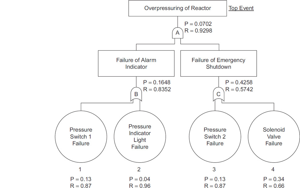
The complete fault tree is shown in Figure 12-14.

Determining the Minimal Cut Sets

Once the fault tree has been fully drawn, a number of computations can be performed. The first computation determines the minimal cut sets (min cut sets). The minimal cut sets are the various sets of events that could lead to the top event. In general, the top event could occur through several different combinations of events. The unique sets of events leading to the top event are the minimal cut sets.

The minimal cut sets are useful for determining the various ways in which a top event could occur. Some of these minimal cut sets have a higher probability than others. For instance, a set involving just two events is more likely than a set involving three events. Similarly, a set involving human interaction is more likely to fail than one involving hardware alone. Based on these simple rules, the minimal cut sets are ordered with respect to failure probability. The higher probability sets are examined carefully to determine whether additional safety systems are required.

The minimal cut sets are determined using a procedure developed by Fussell and Vesely.⁴ The procedure is best described using an example.

⁴J. B. Fussell and W. E. Vesely. “A New Methodology for Obtaining Cut Sets for Fault Trees.” Transactions of the American Nuclear Society 15, no.1 (1972): 262-263.

Example 12-6

Determine the minimal cut sets for the fault tree of Example 12-5.

Solution

The first step in the procedure is to label all the gates using letters and to label all the basic events using numbers. This is shown in Figure 12-14. The first logic gate below the top event is written:

$A$ $A$

AND gates increase the number of events in the cut sets, whereas OR gates lead to more sets. Logic gate A in Figure 12-14 has two inputs: one from gate B and the other from gate C. Because gate A is an AND gate, gate A is replaced by gates B and C:

$A B C$ $A B C$

Gate B has inputs from event 1 and event 2. Because gate B is an OR gate, gate B is replaced by adding a new row below the present row. First, replace gate B by one of the inputs, and then create a second row below the first. Copy into this new row all the entries in the remaining column of the first row:

$\begin{matrix} A B 1 C \\ 2 C \end{matrix}$ $\begin{matrix} A B 1 C \\ 2 C \end{matrix}$

Note that the C in the second column of the first row is copied to the new row.

Next, replace gate C in the first row by its inputs. Because gate C is also an OR gate, replace C by basic event 3 and then create a third row with the other event. Be sure to copy the 1 from the other column of the first row:

$\begin{matrix} A B 1 C 3 \\ 2 C \\ 1 4 \end{matrix}$ $\begin{matrix} A B 1 C 3 \\ 2 C \\ 1 4 \end{matrix}$

Finally, replace gate C in the second row by its inputs. This generates a fourth row:

$\begin{matrix} A B 1 C 3 \\ 2 C 3 \\ 1 4 \\ 2 4 \end{matrix}$ $\begin{matrix} A B 1 C 3 \\ 2 C 3 \\ 1 4 \\ 2 4 \end{matrix}$

The cut sets are then

$\begin{array}{l} 1, 3 \\ 2, 3 \\ 1, 4 \\ 2, 4 \end{array}$ $\begin{array}{l} 1, 3 \\ 2, 3 \\ 1, 4 \\ 2, 4 \end{array}$

This means that the top event occurs as a result of any one of these sets of basic events.

The procedure does not always deliver the minimal cut sets. Sometimes a set might be of the following form:

$1, 2, 2$ $1, 2, 2$

This is reduced to simply 1, 2. On other occasions, the sets might include supersets. For instance,

$\begin{matrix} 1, & 2 \\ 1, & 2, & 4 \\ 1, & 2, & 3 \end{matrix}$ $\begin{matrix} 1, & 2 \\ 1, & 2, & 4 \\ 1, & 2, & 3 \end{matrix}$

The second and third sets are supersets of the first basic set because events 1 and 2 are in common. The supersets are eliminated to produce the minimal cut sets. For this example, there are no supersets.

Quantitative Calculations Using the Fault Tree

The fault tree can be used to perform quantitative calculations to determine the probability of the top event. This is accomplished in two ways.

With the first approach, the computations are performed using the fault tree diagram itself. The failure probabilities of all the basic, external, and undeveloped events are written on the fault tree; then the necessary computations are performed across the various logic gates. Remember that probabilities are multiplied across an AND gate and that reliabilities are multiplied across an OR gate. The computations are continued in this fashion until the top event is reached. Inhibit gates are considered a special case of an AND gate.

The results of this procedure are shown in Figure 12-14. In this figure, the letter “P” represents the probability and “R” represents the reliability. The failure probabilities for the basic events were obtained from Example 12-2.

With the second approach, you use the minimal cut sets. This procedure approximates the exact result only if the probabilities of all the events are small. In general, this result provides a number that is larger than the actual probability. This approach assumes that the probability cross-product terms shown in Equation 12-10 are negligible.

The minimal cut sets represent the various failure modes. For Example 12-6, events 1, 3 or 2, 3 or 1, 4 or 2, 4 could cause the top event. To estimate the overall failure probability, the probabilities from the cut sets are added together. For this case,

$\begin{array}{l} \begin{matrix} P (1 AND 3) & = & (0.13) (0.13) & = 0.0169 \\ P (2 AND 3) & = & (0.04) (0.13) & = 0.0052 \\ P (1 AND 4) & = & (0.13) (0.34) & = 0.0442 \\ P (2 AND 4) & = & (0.04) (0.34) & = 0.0136 \end{matrix} \\ \begin{array}{l} Total & \bar{\begin{array}{l} 0.0799 \end{array}} \end{array} \end{array}$ $\begin{array}{l} \begin{matrix} P (1 AND 3) & = & (0.13) (0.13) & = 0.0169 \\ P (2 AND 3) & = & (0.04) (0.13) & = 0.0052 \\ P (1 AND 4) & = & (0.13) (0.34) & = 0.0442 \\ P (2 AND 4) & = & (0.04) (0.34) & = 0.0136 \end{matrix} \\ \begin{array}{l} Total & \bar{\begin{array}{l} 0.0799 \end{array}} \end{array} \end{array}$

This compares to the exact result of 0.0702 obtained using the actual fault tree. The cut sets are related to each other by the OR function. For Example 12-6, all the cut set probabilities were added. This is an approximate result, as shown by Equation 12-10, because the cross-product terms were neglected. For small probabilities, the cross-product terms are negligible and the addition will approach the true result.

Advantages and Disadvantages of Fault Trees

The main disadvantage of using fault trees is that for any reasonably complicated process the fault tree will be enormous. Fault trees involving thousands of gates and intermediate events are typical. Fault trees of this size require a considerable amount of time, measured in years, to complete.

Furthermore, the developer of a fault tree can never be certain that all the failure modes have been considered. More complete fault trees are usually developed by more experienced engineers.

Fault trees also assume that failures are “hard,” meaning that a particular item of hardware does not fail partially. A leaking valve is a good example of a partial failure. Also, the approach assumes that a failure of one component does not stress the other components, resulting in a change in the component failure probabilities.

Fault trees developed by different individuals are usually different in structure. The different trees generally predict different failure probabilities. This inexact nature of fault trees is a considerable problem. Fault trees developed by experienced risk analysts are much more consistent.

If the fault tree is used to compute a failure probability for the top event, then failure probabilities are needed for all the events in the fault tree. These probabilities are not usually known or are not known accurately.

A major advantage of the fault tree approach is that it begins with a top event. This top event is selected by the user to be specific to the failure of interest. In contrast, in the event tree approach, the events resulting from a single failure might not be the events of specific interest to the user.

Fault trees are also used to determine the minimal cut sets. The minimal cut sets provide enormous insight into the various ways that top events might occur. Some companies adopt a control strategy to have all their minimal cut sets be a product of four or more independent failures. This, of course, increases the reliability of the system significantly.

Software is available for graphically constructing fault trees, determining the minimal cut sets, and calculating failure probabilities. Reference libraries containing failure probabilities for various types of process equipment can also be included.

12-4 Bow-Tie Diagrams

Event trees begin with an initiating event and work toward the top event (induction). By comparison, fault trees begin with a top event and work backward toward the initiating event (deduction). The initiating events are the causes of the incident and the top events are the final outcomes. The two methods are related in that the top event for a fault tree is the initiating event for an event tree. Both are used together to produce a complete picture of an incident, from its initiating causes all the way to its final outcome, including the effects of safeguards. Probabilities and frequencies are attached to these diagrams.

A bow-tie diagram is created by connecting the top event of a fault tree to the initiating event of an event tree, as shown in Figure 12-15. Visually, Figure 12-15 looks like a bow-tie used in clothing.

The Bow-Tie analysis diagram. — **Figure 12-15** Diagram for bow-tie analysis. See Table 1-1 for definitions. (Sources: Adapted from AICHE/CCPS SACHE Faculty Workshop. “Functional Strategy for Protective Functions” (Freeport, TX: Dow Chemical, Freeport, 2016); AICHE Center for Chemical Process Safety. *Guidelines for Enabling Conditions and Conditional Modifiers in Layer of Protection Analysis* (Hoboken, NJ: Wiley Interscience, 2014), p. 79.)

In the Bow-Tie analysis diagram, at the center is the Incident or Loss event. To the left of this event, falling toward the center are: Hazards, Initiating Events, Enabling Conditions, Conditional Modifiers, and Preventive Safeguards. To the right of Incident or Loss event, moving away from the event are: Mitigating Safeguards, Outcomes, and Impact.

The bow-tie diagram is also called barrier analysis since this method identifies safeguards that can prevent and mitigate hazards. It is suitable for the pilot plant, detailed engineering, routine operation, process modification or plant expansion, and incident investigation stages of a process lifetime, as shown in Table 11-3.

The bow-tie diagram provides a good visualization of the relationships between the initiating events, safeguards, and the final consequences. See Section 1-11 for additional details.

The bow-tie diagram can be used to facilitate a range of studies, from simple to complex. On the complex side, it can be used to guide a more detailed quantitative risk analysis (QRA) study, and to clearly display the results. On the simple side, just a portion of the diagram can be used. For example, one can study how the initiating frequencies are affected by different preventive and mitigative safeguards.

The advantages to a bow-tie diagram are that the results are (1) clearly displayed, (2) easily understood, and (3) used to effectively determine the appropriate safeguards to achieve the desired results.

12-5 Quantitative Risk Analysis

Until the late 1990s, quantitative risk analysis (QRA) was the dominant method used to perform risk analysis. QRA is a very rigorous method using source models, dispersion models, and effect models to calculate risk estimates for every possible scenario. The problem with this approach is that the scenarios are typically very numerous, requiring a huge amount of computation to estimate the likelihood and consequences of each scenario.

The major steps of a QRA study are as follows:

Define the initiating events and the incident sequence. For example, a cooling water failure causes a runaway reaction that overpressures the reactor vessel, causing the relief to open, discharging the reactor contents.
Use source models to estimate the discharge rate. For the reactor example, this would require a source model to estimate the discharge rate through the relief. (See Chapter 4.)
Use a dispersion model to estimate the chemical concentrations downwind of the release. (See Chapter 5.)
Estimate the incident consequences for people, environment, and property using effect models. (See Chapter 3.)
Estimate the potential incident frequencies using event trees and fault trees.
Estimate the risk by combining the consequences and frequencies.
Combine the risk estimates for all the scenarios to estimate the overall risk.
Decide if the risk is tolerable. (See Sections 1-9 and 12-7.)

QRA is a complex procedure that requires expertise and a substantial commitment of resources and time. Commercial computer codes are available to assist with these calculations.

12-6 Layer of Protection Analysis⁵

⁵Center for Chemical Process Safety. Layer of Protection Analysis: Simplified Process Risk Assessment, ed. D. A. Crowl. (New York, NY: American Institute of Chemical Engineers, 2001).

In the late 1990s, risk analysts decided that performing a detailed QRA on each of the numerous scenarios was very arduous. The layer of protection analysis (LOPA) method was developed as a simplified QRA. Originally, LOPA was used only by corporate risk analysts, but today it is routinely used by plant process engineers.

LOPA is a semi-quantitative and simplified form of quantitative risk analysis using order of magnitude categories for determining event frequency, consequence severity, and likelihood of failure of safeguards or protection layers. Protection layers are then added to lower the frequency of the undesired consequences. The combined effects of the protection layers and the consequences are then compared against risk tolerance criteria. LOPA is suitable for the conceptual design, pilot plant, detailed engineering, routine operation, and process modification or plant expansion stages of a process lifetime, as shown in Table 11-3.

In LOPA, the consequences and effects are approximated by categories, and both the frequencies and the effectiveness of the protection layers are estimated. The approximate values and categories are selected to provide conservative results. Thus, the results of a LOPA should always be more conservative than those from a much more detailed QRA. If the LOPA results are unsatisfactory or if there is any uncertainty in the results, then a full QRA may be justified.

The most important part of LOPA is to determine the protection layers. For LOPA, the protection layers must be independent protection layers (IPLs). IPLs are a special type of safeguard and must meet all of the following criteria:

Independence—performance of the IPL must not be affected by the initiating cause or the failure of other protection layers.
Functionality—must perform the required response to a specific abnormal condition.
Integrity—must be able to deliver the expected risk reduction.
Reliability—must operate as intended under stated conditions for a specified time period.
Auditability—must be capable of review to determine the adequacy of the IPL.
Access security—must have management systems to reduce the potential for unintentional or unauthorized changes.
Management of change—must have management systems to review, document, and approve any modifications to the IPL.

LOPA does have some limitations:

LOPA is not a scenario identification tool. A method must be available to identify accident scenarios, initiating causes, and safeguards.
LOPA is not a replacement for a detailed QRA. Complex scenarios warrant a QRA.
LOPA requires more time to reach a risk decision than HAZOP or what-if analysis. The value of LOPA for simple decisions is minimal.
Risk comparisons are valid only if (a) the same methods are used to select failure data and (b) comparisons are based on the same risk tolerance criteria.
LOPA cannot generally be compared between organizations due to differences in risk tolerance and LOPA implementation.

The primary purpose of LOPA is to determine whether the process includes sufficient layers of protection against a specific incident scenario. As illustrated in Figure 12-16, many types of protective layers are possible. Figure 12-16 does not include all possible layers of protection, and many of these layers might not be independent. A scenario may require one or many layers of protection, depending on the plant’s complexity and the potential severity of an incident. Note that for a given scenario, only one layer must work successfully for the consequence to be prevented. However, because no layer is perfectly effective, sufficient layers must be added to the process to reduce the risk to a tolerable level.

A diagrammatic illustration of the layers of protection is shown. — **Figure 12-16** Layers of protection, with examples, to lower the frequency of a specific incident scenario. Not all of these are likely to be independent. (Source: Center for Chemical Process Safety. *Layer of Protection Analysis: Simplified Process Risk Assessment*, ed. D. A. Crowl. (New York, NY:
American Institute of Chemical Engineers, 2001).)

In the layers of protection diagram, the inner most layer is the process design, which is constituted of a chemical reactor. The chemical reactor has a monomer input feed and lets out Polymer product. It also has a steam inflow and a cooling water supply at the bottom. The rest of the layers surrounding the Process Design layer, from the innermost to the outermost are as follows: Basic Process Control Systems, Critical Alarms and Human Intervention, Safety Instrumented Functions (SIFs), Physical Protection (Relief Devices), Post-Release Physical Protection (Dikes), Plant Emergency Response, and Community Emergency Response.

The major steps in LOPA are as follows:

Identify a single consequence to screen the scenarios (a method to determine consequence categories is described later in this section).
Identify an incident scenario and cause associated with the consequence (the scenario consists of a single cause–consequence pair).
Identify the initiating event for the scenario and estimate the initiating event frequency (a method to determine the frequency is described later in this section). The initiating cause assumes failure of all the preventive safeguards.
Identify the IPLs available for this particular consequence and estimate the probability of failure on demand (PFD) for each IPL.
Calculate the scenario frequency by combining the initiating event frequency with the probabilities of failure on demand for the IPLs.
Evaluate the risk for tolerability (if not tolerable, additional layers of protection are required).

This procedure is repeated for other consequences and scenarios.

Estimating the LOPA Consequence

In LOPA, the consequences or severity of an incident is estimated using the risk matrix shown in Table 1-14. Here, the consequences are categorized by either human health impact, direct dollar loses due to a fire or explosion or chemical impact. The chemical impact is based on the threshold quantity (TQ) provided in Table 1-15.

Some companies require semi-quantitative or even quantitative measures if the risk is above the company’s threshold criteria. See Section 12-7 for details.

Notice that the LOPA technique does not differentiate between sparsely or densely populated areas for releases. All releases are considered the same risk.

Estimating the LOPA Frequency

When conducting a LOPA study, several methods can be used to determine the frequency. One of the less rigorous methods includes the following steps:

Determine the failure frequency of the initiating event. Typical failure frequencies are provided in Table 12-2.

Table 12-2 Typical Failure Frequency Values Assigned to Initiating Event^a

Initiating event	Frequency range from literature (per year)	Example of a value chosen by a company for use in LOPA (per year)
Pressure vessel residual failure	10^–5 to 10^–7	10^–6
Piping residual failure, 100 m, full breach	10^–5 to 10^–6	10^–5
Piping leak (10% section), 100 m	10^–3 to 10^–4	10^–3
Atmospheric tank failure	10^–3 to 10^–5	10^–3
Gasket/packing blowout	10^–2 to 10^–6	10^–2
Turbine/diesel engine overspeed with casing breach	10^–3 to 10^–4	10^–4
Third-party intervention (e.g., external impact by backhoe or vehicle)	10^–2 to 10^–4	10^–2
Crane load drop	10^–3 to 10^–4/lift	10^–4/lift
Lightning strike	10^–3 to 10^–4	10^–3
Safety valve opens spuriously	10^–2 to 10^–4	10^–2
Cooling water failure	1 to 10^–2	10^–1
Pump seal failure	10^–1 to 10^–2	10^–1
Unloading/loading hose failure	1 to 10^–2	10^–1
Basic process control system (BPCS) instrument loop failure	1 to 10^–2	10^–1
Regulator failure	1 to 10^–2	10^–1
Small external fire (aggregate causes)	10^–1 to 10^–2	10^–1
Large external fire (aggregate causes)	10^–2 to 10^–3	10^–2
LOTO (lock-out/tag-out) procedure failure (overall failure of a multiple element process)	10^–3 to 10^–4/opportunity	10^–3/opportunity
Operator failure (to execute routine procedure; well trained, unstressed,not fatigued)	10^–1 to 10^–3/opportunity	10^–2/opportunity

^aIndividual companies choose their own values, consistent with the degree of conservatism or the company’s risk tolerance criteria. Failure rates can also be greatly reduced by preventive maintenance routines.

Source: Center for Chemical Process Safety. Layer of Protection Analysis, Simplified Process Risk Assessment, ed.D. A. Crowl. (New York, NY: American Institute of Chemical Engineers, 2001).

Adjust this frequency to include the demand. For example, a reactor failure frequency is divided by 12 if the reactor is used only 1 month during the entire year. The frequencies are also adjusted (reduced) to include the benefits of preventive maintenance. If, for example, a control system is given preventive maintenance 4 times each year, then its failure frequency is divided by 4.

Adjust the failure frequency to include the PFD for each independent layer of protection. Table 12-3 contains typical PFD values for passive IPLs. Table 12-4 contains PFDs for active IPLs and human interactions.

Table 12-3 PFDs (per year) for Passive IPLs

Passive IPLs	Comments (assuming an adequate design basis, inspections, and maintenance procedures)	PFDs from industry^a	PFDs from CCPS^a
Dike	Reduces the frequency of large consequences (widespread spill) of a tank overfill, rupture, spill, etc.	10^–2 to 10^–3	10^–2
Underground drainage system	Reduces the frequency of large consequences (widespread spill) of a tank overfill, rupture, spill, etc.	10^–2 to 10^–3	10^–2
Open vent(no valve)	Prevents overpressure	10^–2 to 10^–3	10^–2
Fireproofing	Reduces rate of heat input and provides additional time for depressurizing, firefighting, etc.	10^–2 to 10^–3	10^–2
Blast wall or bunker	Reduces the frequency of large consequences of an explosion by confining blast and by protecting equipment, buildings, etc.	10^–2 to 10^–3	10^–3
Inherently safer design	If properly implemented, can eliminate scenarios or significantly reduce the consequences associated with a scenario	10^–1 to 10^–6	10^–2
Flame or detonation arrestors	If properly designed, installed, and maintained, can eliminate the potential for flashback through a piping system or into a vessel or tank	10^–1 to 10^–3	10^–2

^aCenter for Chemical Process Safety. Layer of Protection Analysis, Simplified Process Risk Assessment, ed. D. A. Crowl. (New York, NY: American Institute of Chemical Engineers, 2001).

Table 12-4 PFDs (per year) for Active IPLs and Human Actions

Active IPL or human action	Human action [assuming an adequate design basis, inspections, maintenance procedures (active IPLs), adequate documentation, training, and testing procedures]	PFDs from industry^a	PFDs from CCPS^a
Relief valve	Prevents system from exceeding specified overpressure. Effectiveness of this device is sensitive to service and experience.	10^–1 to 10^–5	10^–2
Rupture disc	Prevents system from exceeding specified overpressure. Effectiveness of this device can be sensitive to service and experience.	10^–1 to 10^–5	10^–2
Basic process control system (BPCS)	Can be credited as an IPL if not associated with the initiating event being considered. See IEC (1998, 2001).^b,c	10^–1 to 10^–2	10^–1
Safety instrumented functions (SIF)	See IEC 61508 (IEC, 1998) and IEC 61511 (IEC, 2001) for life-cycle requirements and additional discussion.^b,c
Human action with 10-min response time	Simple well-documented action with clear and reliable indications that the action is required.	1 to 10^–1	10^–1
Human action with 40-min response time	Simple well-documented action with clear and reliable indications that the action is required.	10^–1 to 10^–2	10^–1

^aCenter for Chemical Process Safety. Layer of Protection Analysis, Simplified Process Risk Assessment, ed. D. A. Crowl. (New York, NY: American Institute of Chemical Engineers, 2001).

^bInternational Electrotechnical Commission. IEC 61508, Functional Safety of Electrical/Electronic/Programmable Electronic Safety-Related Systems, Parts 1–7 (Geneva, Switzerland: International Electrotechnical Commission, 1998).

^cInternational Electrotechnical Commission. IEC 61511, Functional Safety Instrumented Systems for the Process Industry Sector, Parts 1–3 (Geneva, Switzerland: International Electrotechnical Commission, 2004).

Estimating frequencies from historical data can be challenging because there may be protection layers in place influencing the failure rates. The LOPA team needs to clarify what is included in the frequencies. For instance, if a company requires a high-level interlock on every storage tank, should that company consider a high-level interlock to be a protection layer or merely the company’s requirement for the initiating event frequency? The procedure must ensure that common protection layers are not “double counted.” This problem emphasizes the reason for including experienced team members for LOPA.

The frequency of a consequence of a specific scenario endpoint is computed using

$\begin{matrix} f_{i}^{c} = f_{i}^{I} \times Π_{j = 1}^{i} {P F D}_{i j} & (12 - 31) \end{matrix}$ $\begin{matrix} f_{i}^{c} = f_{i}^{I} \times Π_{j = 1}^{i} {P F D}_{i j} & (12 - 31) \end{matrix}$

where

$f_{i}^{c}$ $f_{i}^{c}$ is the mitigated consequence frequency for a specific consequence C for an initiating event i,

$f_{i}^{I}$ $f_{i}^{I}$ is the initiating event frequency for the initiating event i, and

PFD_ij is the probability of failure of the jth IPL that protects against the specific consequence and the specific initiating event i.

When there are multiple scenarios with the same consequence, each scenario is evaluated individually using Equation 12-31. The frequency of the consequence is subsequently determined using

$\begin{matrix} f^{c} = \sum_{i = 1}^{I} f_{i}^{c} & (12 - 32) \end{matrix}$ $\begin{matrix} f^{c} = \sum_{i = 1}^{I} f_{i}^{c} & (12 - 32) \end{matrix}$

where

$f_{i}^{c}$ $f_{i}^{c}$ is the frequency of the Cth consequence for the ith initiating event and

I is the total number of initiating events for the same consequence.

Example 12-7 shows that the failure frequency is easily determined using LOPA.

Example 12-7

Determine the consequence frequency for a cooling water failure if the system is designed with two IPLs. The IPLs are human interaction with a 10-min response time and a basic process control system (BPCS).

Solution

The frequency of a cooling water failure is taken from Table 12-2; that is, $f_{i}^{I} = 10^{- 1} / yr$ $f_{i}^{I} = 10^{- 1} / yr$ . The PFDs are estimated from Tables 12-3 and 12-4. The PFD for the BPCS is 10^–1 and the human response PFD is 10^–1. The consequence frequency is found using Equation 12-31:

$\begin{matrix} f_{i}^{C} & = f_{i}^{I} \times \prod_{j = 1}^{i} PF D_{i j} \\ = (10^{- 1} failures/yr) \times (10^{- 1}) \times (10^{- 1}) = 13^{- 3} failures/yr \end{matrix}$ $\begin{matrix} f_{i}^{C} & = f_{i}^{I} \times \prod_{j = 1}^{i} PF D_{i j} \\ = (10^{- 1} failures/yr) \times (10^{- 1}) \times (10^{- 1}) = 13^{- 3} failures/yr \end{matrix}$

The PFD concept is also used when designing emergency shutdown systems called safety instrumented functions (SIFs). A SIF achieves low PFD values in the following ways:

Using redundant sensors and final redundant control elements
Using multiple sensors with voting systems and redundant final control elements
Testing the system components at specific intervals to reduce the PFD by detecting unrevealed failures
Using a deenergized trip system (i.e., a relayed shutdown system)

Three safety integrity levels (SILs) are generally accepted in the chemical process industry for emergency shutdown systems:

SIL 1 (PFD = 10^–1 to 10^–2): These SIFs are usually implemented with a single sensor, a single logic solver, and a single final control element, and they require periodic proof testing.
SIL 2 (PFD = 10^–2 to 10^–3): These SIFs are typically fully redundant, including the sensor, logic solver, and final control element, and they require periodic proof testing.
SIL 3 (PFD = 10^–3 to 10^–4): These SIFs are typically fully redundant, including the sensor, logic solver, and final control element; the system requires careful design and frequent validation tests to achieve the low PFD figures. Many companies find that they have a limited number of SIL 3 systems because of the high cost typically associated with this architecture.

IPLs typically have a well-defined hierarchy. Figure 12-17 shows a typical hierarchy, along with the response limits for each layer. This hierarchy includes the following layers:

Basic Process Control System (BPCS): The BPCS normally keeps the process under control. If a process deviation exceeds the control limits, then an alarm alerts the operator.
Operator Response to an Alarm: The operator should respond but may not.

Figure 12-17 Typical hierarchy of independent protection layers (IPLs). (Source: Adapted from AICHE/CCPS SACHE Faculty Workshop. “Protective Functions” (Freeport, TX: Dow Chemical, June 2016).)

A figure depicts the hierarchy and their response limits with respect to Independent Protection Layers. The Typical layers of protection from bottom to top are: Process Control BPCS, Operator Responses to Alarms, BPCS (Shut the system down), SIS, and PRD (which also constitutes the LOPC). The response limits of the layers are depicted using a curve. When the issue is addressed in the Operator Responses to Alarm layer or the BPCS Shutdown layer, the process moves back to Process Control BPCS. When the issue is addressed in the SIS layer, the process is led to Operator Responses to Alarm layer. When the issue is address in the PRD layer, the process still remains in the same layer. When the issue is left unaddressed, it leads to Bad Outcome.
BPCS: If the operator doesn’t respond, then the BPCS has a high-high level interlock to shut the system down.
Safety Instrumented System (SIS): The SIS is separate from the BPCS and consists of multiple Safety Instrumented Functions (SIF) designed to achieve a specific SIL. The SIS consists of the SIFs and all associated field sensors, logic solver, final control elements, etc. The purpose of the SIF is to isolate the threat and put the unit in a safe state— this may or may not include shutting down the process.
Pressure Relief Device (PRD): If the SIS doesn’t work, then the PRD mitigates the pressure within the process equipment.
Loss of Primary Containment (LOPC): If the PRD does not have a secondary containment system, the process material is discharged to the atmosphere, resulting in an LOPC.
Bad Outcome: If this last IPL fails, then a major incident occurs, such as a ruptured vessel or ruptured pipeline.

An enabling condition is a probability that adjusts the initiating event frequency to account for the time-at-risk due to the presence of specific circumstances. The enabling condition probability adjusts the initiating frequency to give a frequency without IPLs. Examples included the following probabilities:

The probability that a reactor is used for a hazardous reaction (e.g., one week in a month or a probability of 0.25)
The probability that a reactor is in a hazardous condition (e.g., when it is in a recycle mode that occurs only 10 hours per year or a probability of 10/(52 × 7 × 24) or 10/8736 or 0.0011)
The hazardous condition occurs only 3 weeks each year, giving a probability of 0.058.

A conditional modifier is a probability that adjusts the initiating event frequency to account for the probability of a specific hazardous event. The conditional modifier probability adjusts the LOPA initiating frequency (together with enabling conditions) to give a frequency without IPLs. Examples of conditional modifiers include (1) probability of a hazardous atmosphere, (2) probability of ignition, (3) probability of an explosion, (4) probability of the presence of personnel, (5) probability of injury or fatality, and (6) probability of a financial loss.

Enabling conditions and conditional modifiers are primarily based on a specific company’s experience and represent the fraction of the time the equipment is in a hazardous condition. Some examples include the following factors:

A company has found that the temperature in the hazardous region exceeds the flash point for 4 months per year, giving a probability of 0.333.
A company’s historical experience indicates that ignition of a flammable material release will occur once in every 10 spills, giving a probability of 0.1.
The fraction of the time (probability) that a vessel has a pressure when a deflagration pressure exceeds the ultimate strength of the vessel.
The fraction of the time that people are in the affected area.

The LOPA method offers many advantages:

Requires less time than a QRA
Helps resolve conflicts in decision making by providing a consistent, simplified framework to make better risk decisions
Improves hazard evaluations by providing a tool to arrive at risk decisions quickly
Improves scenario identification by providing more precise cause–consequence pairs
Provides a means to compare risk between process units
Provides a more defensible comparative risk judgment than do qualitative methods
Helps decide if the risk is “as low as reasonably possible” (ALARP)
Helps identify operations and practices that were thought to have sufficient safeguards
Provides a clear, functional specification of IPLs
Helps focus on IPLs
Can be applied by process engineers at the plant level

Example 12-8

Perform a LOPA analysis for two of the following major scenarios involving a storage and reactor vessel. The flammable liquid is maintained above its normal boiling point temperature by its own vapor pressure. The threshold quantity (TQ) for the release of this liquid is 1000 lb. The two scenarios are:

A fire external to a storage vessel containing 50,000 pounds of the liquid. The probability of personnel being in the affected area is 0.50. Multiple employee fatalities are likely from this incident. A dike exists around the storage vessel to contain the liquid and fire.
A control loop failure for a reactor vessel containing 20,000 pounds of the liquid. This results in a runaway reaction, with a major release of the reactor contents through a relief device. The reactor is operated 100 days per year. The material released is expected to be 15 times the TQ.

Solution

The LOPA results are shown in Table 12-5. The initiating event frequencies are from Table 12-2.

Table 12-2 is used to estimate the initiating event frequency. For scenario 1 this is once every 100 years and for scenario 2 it is once every 10 years.
The risk matrix from Table 1-14 is used to estimate the severity level. For scenario 1, since multiple employee fatalities are expected, this is classified as “Catastrophic” and the safety severity level is 4. For scenario 2, since the release is 15 times the TQ, the incident is classified as “Very Serious” with a safety severity level of 3.
Next, the likelihood is determined from the risk matrix of Table 1-14. For scenario 1, since this occurs once every 100 years, it is classified as “Improbable.” Scenario 2 is expected to occur once every 10 years, so it is classified as “Unlikely.”
The severity level and likelihood are combined using Table 1-14 to determine the risk level. For both scenarios 1 and 2, this is risk level B. From the legend at the bottom of Table 1-14, risk level B is an undesirable risk and requires that additional safeguards must be implemented within 3 months.
The severity level from Step 3 is used with Table 1-14 to determine the target mitigated event frequency (TMEF). For scenario 1 this is 10^–6 per year and for scenario 2 this is 10^–5 per year.
For scenario 1 there are no enabling conditions since the storage vessel contains the flammable liquid all the time. For scenario 2 the reactor is operated only 100 days per year which is 100/365 = 0.27.
The conditional modifier for scenario 1 is given as 0.5 for people being present in the area only 50% of the time. There are no conditional modifiers for scenario 2.
The initiating event frequency from row 1 is then multiplied by the enabling conditions (row 6) and the conditional modifiers (row 7) to estimate the adjusted initiating event (IE) frequency in row 8.
This row shows the existing layers of protection for both scenarios and the probability of failure on demand (PFD) from Table 12-4.
Row 8 is multiplied by row 9 to arrive at the frequency with the existing layers of protection.

Row 10 is divided by the TMEF from row 5 to arrive at row 11. Row 11 represents the additional layers of protection required to meet the TMEF. Scenario 1 would require a single SIL 2 to achieve this. Scenario 2 would require a SIL 3. Other combinations of SIL levels or additional equipment from Table 12-4 could be used.

Table 12-5 LOPA for Example 12-8

LOPA worksheet	Scenario 1	Scenario 2
Description of event	Large external fire to storage vessel	Reactor runaway—major release
Initiating event (cause) Initiating event (IE) frequency (Table 12-2)	External fire 10^–2/yr = once/100 years	BPCS failure 10^–1/yr = once/10 years
Severity level (Table 1-14)	CATASTROPHIC due to multiple employee fatalities.	VERY SERIOUS due to the TQ release.
Likelihood (from 1 and Table 1-14)	100 years = IMPROBABLE	10 years = UNLIKELY
Risk level (from 2 and 3 and Table 1-14)	B	B
Target mitigated event frequency (TMEF) (Table 1-14)	10^–6/yr	10^–5/yr
Enabling conditions	N/A	Probability of 100/365 = 0.27
Conditional modifiers	Probability of 0.5	None
Adjusted IE frequency (Multiply 1 × 6 × 7)	5 × 10^–3/yr	2.7 × 10^–2/yr
Existing layers of protection (type and PFD from Table 12-3 )	Dike 10^–2/yr	None
Frequency with existing layers of protection: (Multiply 8 × 9)	5 × 10^–5/yr	2.7 × 10^–2/yr
Additional layers of protection required (Divide 5 by 10)	2.0 × 10^–2	3.7 × 10^–4

12-7 Risk Assessment

Risk assessment involves applying the estimated risk from risk analysis to make decisions. Usually this requires a method to decide if the risk is tolerable. Risk tolerance is discussed in general in Section 1-9. Most companies have established guidelines for risk tolerance.

Consequence versus Frequency Plot

The simplest method for determining risk tolerance is shown in Figure 12-18. The consequences are plotted versus the frequency, and a boundary is drawn between acceptable and not acceptable risk. Note that tolerable risk occurs with either low-frequency or low-consequence events.

A graph portrays the simplest method to determine risk tolerance. — **Figure 12-18** General description of tolerable risk.

A plot of Consequence versus Time shows aids in the determination of tolerable risk. The plot is a concave up, gradually decreasing curve. The region below the curve is labeled "Acceptable." The region above the curve is labeled "Not Acceptable."

Individual Risk: Risk Contours

Individual risk is the risk to an individual person in the vicinity of a hazard. A plot showing individual risk contours is shown in Figure 12-19.

A figure depicts the risk contours. — **Figure 12-19** Individual risk contours. The contours have units of 1/year, where the number is the risk of fatality per year to an individual located on the spot 24 hours per day per year.

In the risk contours plot, four contours are drawn, for the values from the innermost to the outermost as 10 to the power of negative 4, 10 to the power of negative 5, 10 to the power of negative 6, and 10 to the power of negative 7. The innermost location is Plant and the outermost location is Community.

The procedure for determining the individual risk contours is as follows:

Identify all the incidents and incident outcome cases.
Estimate the frequency for all incident outcome cases.
Determine the effect zone and probability of fatality at every location for all incident outcome cases.
Estimate the individual risk at every location by summing the risk for all incident outcome cases.
Plot individual risk estimates on the map.
Draw individual risk contours connecting points of equal risk.

Societal Risk: F-N Plots

Societal risk is a measure of risk to a group of people. An F-N plot is one way to show societal risk. The F is the cumulative frequency of experiencing N or more fatalities. A typical F-N curve is shown in Figure 12-20.

Societal risks are plotted using F-N curves. — **Figure 12-20** F-N curve showing societal risk tolerance curves for several countries.

A graph plots the societal risks across various countries using the f-N curve. The horizontal axis represents N, Fatalities, ranging from 1 to 1000 in increments of multiples of 10. The vertical axis represents F, Cumulative Frequency of N or More (Fatalities/Year), ranging from 10 to the power of negative 9 to 10 to the power of negative 1, in increments of multiplies of 10. The graph infers the following data. All plots are decreasing linear curves, that is, as N increases, F decreases. For country 'A,' when N equals 1, F is 10 to the power of negative 2; similarly, the rest of the values are (10, 10 to the power of negative 3), (100, 10 to the power of negative 4), and (1000, 10 to the power of negative 5). For country B, when N equals 1, F equals 10 to the power of negative 3; similarly, the rest of the values are (10, 10 to the power of negative 5), (100, 10 to the power of negative 7), and (1000, 10 to the power of negative 9). For country C, when N equals 1, F equals 10 to the power of negative 4; similarly, the rest of the values are (10, 10 to the power of negative 5), (100, 10 to the power of negative 6), and (1000, 10 to the power of negative 7). For country D, when N equals 1, F equals 10 to the power of negative 4.5; similarly, the rest of the values are (10, 10 to the power of negative 6), (100, 10 to the power of negative 7.5), and (1000, 10 to the power of negative 9). For country E, when N equals 1, F equals 10 to the power of negative 5; similarly, the rest of the values are (10, 10 to the power of negative 6), (100, 10 to the power of negative 7), and (1000, 10 to the power of negative 8). The region below the last line plotted is labeled Broadly Tolerable. The region above the first line plotted at the top is labeled Broadly Unacceptable.

An F-N curve is drawn using the following procedure:

Identify all incidents and incident outcome cases.
Estimate the frequency for each incident outcome case. This is done using any number of methods presented in this chapter.
Estimate the impact zones and the probability of fatality at every location in the effect zone. This is done using source models (Chapter 4), dispersion models (Chapter 5), and effect models (Chapter 3).
Superimpose the impact zone for each incident outcome case over the population distribution.
Determine the total number of fatalities (N) for each incident outcome case.
Create the F-N plot using the results of step 5 and the procedure shown in Example 12-9.

Figure 12-20 contains several F-N plots for tolerable risk from several countries. The plots are identified as follows:

A: United Kingdom’s Health Safety Executive (HSE) Criteria—Maximum tolerable societal risk
B: Dutch—Maximum tolerable societal risk
C: U.K. HSE—Negligible risk to workers and public
D: New South Wales—Negligible societal risk
E: Hong Kong—Acceptable societal risk

Example 12-9

Use the data provided in Table 12-6 to draw an F-N curve.

Table 12-6 Data for an F-N Curve

Incident outcome case	Frequency, F_i (per year)	Estimated number of fatalities, N
1	1 × 10^–6	13
2	1 × 10^–3	0
3	1 × 10^–5	6
4	1 × 10^–5	3
5	1 × 10^–4	1

Solution

The incident outcome case with the smallest number of fatalities is selected first. This is case 5, which has one fatality. Case 2 is not selected because it has zero fatalities. Next, all incident outcome cases with one or more fatalities are selected. These are cases 1, 3, 4, and 5. The frequencies for these cases are added together to create the top entry in Table 12-7.

Table 12-7 F-N Analysis for Example 12-9

Estimated Number of Fatalities, N	Incident Outcome Cases Included	Total Frequency F_N (per year)
1+	1, 3, 4, 5	F₁ + F₃ + F₄ + F₅ = 1.2 × 10^–4
3+	1, 3, 4	F₁ + F₃ + F₄ = 2.1 × 10^–5
6+	1, 3	F₁ + F₃ = 1.1 × 10^–5
13+	1	F₁ = 1.0 × 10^–6
>13	None	0

Next, the case with the next highest number of fatalities is selected. This is case 4, with three fatalities. The frequencies for all cases with three or more fatalities are added together, as shown in Table 12-7.

This procedure is repeated for 6+, 13+, and greater than 13 fatalities. The results are shown in Table 12-17.

The data are plotted in Figure 12-21. The results of Figure 12-21 are extrapolated to N = 1. The vertical lines are drawn at the actual number of fatalities. Note that the results exceed many of the societal risk criteria in Figure 12-20.

An F-N curve is plotted based on the given data set. — **Figure 12-21** *F-N* curve for Example 12-9.

An F-N analysis of the given data-set is presented as a graph. The horizontal axis represents Number of Fatalities, N ranging from 1 to 100 in increments of multiples of 10. The vertical axis represents Frequency of N or More Fatalities, per year, ranging from 10 to the power of negative 6 to 10 to the power of negative 3 in increments of multiples of 10. The plot infers the following data. When N equals 1 to 3, F equals 1.2 times 10 to the power of negative 4. When N equals 3 to 5, F equals 2 times 10 to the power of negative 5. When N equals 6 to 12, F equals 10 to the power of negative 5. When N is greater than 13, F equals 0. Note: the values are approximate.

Problems

12-1. For the reactor shown in Figure 12-5, sketch a fault tree and determine the overall failure rate, the failure probability, the reliability, and the MTBF.

12-2. For the reactor shown in Figure 12-5, sketch a fault tree with redundant alarm and shutdown loops, and determine the overall failure rate, the failure probability, the reliability, and the MTBF.

12-3. For the figure and failure rates shown below, determine for the top event the probability of failure, the reliability, and the MTBF.

A fault tree diagram with the top event as Tank Overflows is given.

Faults per year, μ, for the given basic events:

Basic event	Faults per year
1	0.6
2	1.1
3	3.7
4	1.7
5	2.0
6	1.4
7	0.42

12-4. Determine the minimum cut sets for the fault tree provided in Problem 12-3.

12-5. Modify the event tree of Figure 12-9 to determine the runaways per year if the loss of cooling initiating event is reduced to 0.02 occurrence per year.

12-6. Modify the event tree of Figure 12-11 to determine the runaways per year if the loss of cooling initiating event is reduced to 0.80 occurrence per year.

12-7. A toxic liquid is pumped into a storage vessel. The vessel is equipped with a high-level sensor to stop the flow and sound an alarm if the level is too high. If the level sensor and alarm fail, the vessel will overflow and the toxic material will be released into the operating environment. Use the LOPA method to determine if this system requires additional safeguards. Assume a threshold quantity for the liquid of 5 lb. The pumping rate is 1 lb/min and it will take 20 min for the operator to notice the spill and stop the flow manually. Make suggestions for improvement if additional safeguards are required.

12-8. A reactor experiences trouble once every 16 months. The protection device fails once every 25 years. Inspection takes place once every month. Calculate the unavailability, the frequency of dangerous coincidences, and the MTBC.

12-9. A starter is connected to a motor that is connected to a pump. The starter fails once in 50 years and requires 2 hours to repair. The motor fails once in 20 years and requires 36 hours to repair. The pump fails once per 10 years and requires 4 hours to repair. Determine the overall failure frequency, the probability that the system will fail in the coming 2 years, the reliability, and the unavailability for this system.

12-10. If a regulator has a consequence frequency of 10^–1 failure/yr, what will be the frequency if this regulator is given preventive maintenance once per month?

12-11. Draw an F-N curve using the following data:

Incident outcome case	Frequency, F_i (per year)	Estimated number of fatalities, N
1	1 × 10^–6	20
2	1 × 10^–4	5
3	1 × 10^–5	7
4	1 × 10^–5	3
5	1 × 10^–4	2

12-12. The peak overpressure expected as a result of the explosion of a tank in a plant is approximated by the following equation:

$log P = 6.0 - 1.8 log r$ $log P = 6.0 - 1.8 log r$

where P is the overpressure in psi and r is the distance from the blast in feet. The plant employs 50 people who work in an area from 10 to 500 ft from the blast. Assume that the population density is constant in the work area.

Estimate the fraction of fatalities at 10, 100, 250, and 500 ft using a probit equation.
Calculate the individual risk at each location in part (a) in yr^–1. Assume a frequency of the initiating event of 10^–4 per year.
Plot the risk contours.

Additional homework problems are available in the Pearson Instructor Resource Center.

..................Content has been hidden....................

You can't read the all page of ebook, please click here login for view all page.

Table of Contents for
Chapter 12. Risk Analysis and Assessment

Chapter 12. Risk Analysis and Assessment

12-1 Review of Probability Theory

Interactions between Process Units

Revealed and Unrevealed Failures

Probability of Coincidence

Redundancy²

Common-Cause Failures

12-2 Event Trees

12-3 Fault Trees

Determining the Minimal Cut Sets

Quantitative Calculations Using the Fault Tree

Advantages and Disadvantages of Fault Trees

12-4 Bow-Tie Diagrams

12-5 Quantitative Risk Analysis

12-6 Layer of Protection Analysis⁵

Estimating the LOPA Consequence

Estimating the LOPA Frequency

12-7 Risk Assessment

Consequence versus Frequency Plot

Individual Risk: Risk Contours

Societal Risk: F-N Plots

Suggested Reading

Problems

Table of Contents for Chapter 12. Risk Analysis and Assessment

Create new playlist

Sign In

Sign Up

Chapter 12. Risk Analysis and Assessment

12-1 Review of Probability Theory

Interactions between Process Units

Revealed and Unrevealed Failures

Probability of Coincidence

Redundancy2

Common-Cause Failures

12-2 Event Trees

12-3 Fault Trees

Determining the Minimal Cut Sets

Quantitative Calculations Using the Fault Tree

Advantages and Disadvantages of Fault Trees

12-4 Bow-Tie Diagrams

12-5 Quantitative Risk Analysis

12-6 Layer of Protection Analysis5

Estimating the LOPA Consequence

Estimating the LOPA Frequency

12-7 Risk Assessment

Consequence versus Frequency Plot

Individual Risk: Risk Contours

Societal Risk: F-N Plots

Suggested Reading

Problems

Table of Contents for
Chapter 12. Risk Analysis and Assessment

Redundancy²

12-6 Layer of Protection Analysis⁵