Chapter 4. Source Models

Search in book...
Toggle Font Controls
Create new playlist

Name your new playlist

Playlist description (optional)
Sign In

Email address

Password

Forgot Password?

or

Continue with Facebook

Continue with Google
Sign Up

Full Name

Email address

Confirm Email Address

Password

or

Continue with Facebook

Continue with Google

Chapter 4. Source Models

The learning objectives for this chapter are to:

Explain why and how source models are used in risk assessment.
Describe simple source models used for liquids and gases: holes, pipe flow, and liquid pools.
Describe more complex source models: holes in tanks.
Describe more complex source models: evaporation and flashing or boiling liquids.
Distinguish between realistic and worst-case releases.
Perform conservative analysis.

Most incidents in chemical plants result in spills of toxic, flammable, or explosive materials. Source models are an important part of the consequence modeling procedure shown in Figure 4-1. Figure 4-1 also identifies the particular chapters in this book that are related to the topics shown. Additional information is provided elsewhere.¹

¹Center for Chemical Process Safety. Guidelines for Consequence Analysis of Chemical Releases (New York, NY: American Institute of Chemical Engineers, 1999).

A flowchart depicts the consequence model. — **Figure 4-1** Consequence analysis procedure. (Source: Center for Chemical Process Safety. *Guidelines for Consequence Analysis for Chemical Releases* (New York, NY: American Institute of Chemical Engineers, 1999).)

A flowchart of consequence analysis procedure is shown. The flow starts with the selection of a release incident. From there, the process leads to the selection of source model (chapter 4) and dispersion model (chapter 5). A condition, Flammable or Toxic is shown. If flammable, selection of fire and explosion model (chapter 6). If toxic, selection of effect model (chapter 2) with the migration factors. The process ends with the consequence model.

Many incidents result in the loss of containment of material from the process. These materials may have hazardous properties, which could include toxic properties and energy content. Typical incidents might include the rupture or break of a pipeline, a hole in a tank or pipe, runaway reaction, or fire external to the vessel.

Once the incident is identified, source models are selected to describe how materials are discharged from the process. The source model provides a description of the rate of discharge,the total quantity discharged (or total time of discharge), and the state of the discharge (that is solid, liquid, vapor, or a combination). A dispersion model is subsequently used to describe how th material is transported downwind and dispersed to some concentration levels (discussed further in Chapter 5). For releases of flammable materials, fire and explosion models convert the source model information on the release into energy hazard potentials, such as thermal radiation and explosion overpressures (discussed further in Chapter 6). Effect models convert these incident-specific results into effects on people (injury or death) and structures, as described in Chapter 2. Environmental impacts could also be considered, but we do not do so here.

4-1 Introduction to Source Models

Source models are constructed from fundamental or empirical equations representing the physical and chemical processes occurring during the release of materials. For a reasonably complex plant, many source models are needed to describe the release. Some development and modification of the original models is usually required to fit the specific situation.

In many cases, the results are only estimates because the physical properties of the materials are not adequately characterized or because the physical processes themselves are not completely understood. If uncertainty exists, the parameters should be selected to maximize the release rate and quantity. This approach ensures that a design is conservative (discussed further in Sections 4-9 and 4-10).

Release mechanisms are classified into wide- or limited-aperture releases, where apertures are holes and cracks in tanks and pipes, leaks in flanges, valves, and pumps, and severed or ruptured pipes and tanks. In the limited-aperture case, material is released at a slow enough rate that upstream conditions are not immediately affected—the assumption of constant upstream pressure is frequently valid. In the wide-aperture case, a large hole develops in the process unit, releasing a substantial amount of material in a short time. An example is the overpressuring and rupture of a storage tank.

Limited-aperture releases are conceptualized in Figure 4-2. Relief valves, designed to prevent the overpressuring of tanks and process vessels, are also potential sources of released material.

A diagram related to the source model depicts the types of aperture releases. — **Figure 4-2** Various types of limited-aperture releases.

A figure shows the parts of the limited-aperture releases. The following parts are marked in the figure: Crack, Relief valve, ruptured (or severed) pipe, pump (body and seals), flange, hole, and pipe connection.

Figure 4-3 shows how the physical state of the material affects the release mechanism. For gases or vapors stored in a tank, a leak results in a jet of gas or vapor. For liquids, a leak below the liquid level in the tank results in a stream of escaping liquid. If the liquid is stored under pressure above its atmospheric boiling point, a leak below the liquid level will result in a stream of liquid flashing partially into vapor. Small liquid droplets or aerosols might also form from the flashing stream, with the possibility of transport away from the leak by wind currents. A leak in the vapor space above the liquid can result in either a vapor stream or a two-phase stream composed of vapor and liquid.

The ejection of vapor and liquid in different states is illustrated via two diagrams. — **Figure 4-3** Vapor and liquid are ejected from process units in either single- or two-phase states.

A pair of diagrams shows the ejection of Vapor and Liquid in either single or two phase states. The first diagram shows a process unit which stores gas or vapor in its tank. The gas or vapor leaks from the tank. The second diagram shows a vapor or liquid stored in a tank. The vapor or two-phase vapor/liquid leaks from a hole at the top. The liquid or liquid flashing into vapor, leaks from a hole at the bottom.

Several basic source models are used repeatedly and will be developed in detail here:

Flow of liquid through a hole
Flow of liquid through a hole in a tank
Flow of liquids through pipes
Flow of gases or vapor through holes
Flow of gases or vapor through pipes
Flashing liquids
Liquid pool evaporation or boiling

Many other incidents—such as tank overflow, catastrophic failure, excessive heating, and so forth—can be described using source models. Other source models, specific to certain materials, are introduced in subsequent chapters.

4-2 Flow of Liquid through a Hole

A mechanical energy balance describes the various energy forms associated with flowing fluids:

$\begin{matrix} \int \frac{d P}{ρ} + Δ (\frac{{\bar{u}}^{2}}{2 α g_{c}}) + \frac{g}{g_{c}} Δ z + F = - \frac{W_{s}}{\dot{m}} & (4-1) \end{matrix}$

where

P is the pressure (force/area),

ρ is the fluid density (mass/volume),

ū is the average instantaneous velocity of the fluid (length/time²),

g_c is the gravitational constant (length mass/force time²),

α is the unitless velocity profile correction factor with the following values:
α = 0.5 for laminar flow, α = 1.0 for plug flow, andα approaches 1.0 for turbulent flow,

g is the acceleration due to gravity (length/time²),

z is the height above datum (length),

F is the net frictional loss term (length force/mass),

W_s is the shaft work (force length/time), defined as the positive work done by the system on the surroundings, and

$\dot{m}$ is the mass flow rate (mass/time).

The Δ function represents the final minus the initial state.

For incompressible liquids, the density is constant, and

$\begin{matrix} \int \frac{d P}{ρ} = \frac{Δ P}{ρ} & (4-2) \end{matrix}$

Consider a process unit that develops a small hole, as shown in Figure 4-4. The pressure energy of the liquid contained within the process unit is converted to kinetic energy as the fluid escapes through the hole. Frictional forces between the moving liquid and the wall of the leak convert some of the kinetic energy of the liquid into thermal energy, resulting in a reduced velocity.

The leakage of liquid through a hole in a process unit is illustrated via a diagram. — **Figure 4-4** Liquid escaping through a hole in a process unit. The energy of the liquid resulting from its pressure in the vessel is converted to kinetic energy, with some frictional flow losses in the hole.

A figure illustrates the leakage of liquid through a hole in a process unit. The pressurized liquid within the process unit leaks through a hole, into the external surroundings. Various parameters of the pressurized liquid are, P equals P subscript g, u overbar subscript 1, equals 0, delta z equals 0, and W subscript s, equals 0. Various parameters of the external surroundings are, P equals 1 atmosphere and u overbar subscript 2, equals u overbar. A formula below reads as follows. Q subscript m, equals A times C subscript o, times square root of, 2 times pi times g subscript c, times P subscript g. Here, pi equals liquid density and A equals leak area.

For this limited-aperture release, assume a constant gauge pressure P_g within the process unit. The external pressure is atmospheric, so ΔP = P_g. The shaft work is zero, and the velocity of the fluid within the process unit is assumed negligible. The change in elevation of the fluid during the discharge through the hole is also negligible, so Δz = 0. The frictional losses in the leak are approximated by a constant discharge coefficient C_l, defined as

$\begin{matrix} - \frac{Δ P}{ρ} - F = C_{1}^{2} (- \frac{Δ P}{ρ}) & (4-3) \end{matrix}$

The modifications are substituted into the mechanical energy balance (Equation 4-1) to determine ū, the average discharge velocity from the leak:

$\begin{matrix} \bar{u} = C_{1} \sqrt{α} \sqrt{\frac{2 g_{c} P_{g}}{ρ}} & (4-4) \end{matrix}$

A new discharge coefficient C₀ is defined as

$\begin{matrix} C_{o} = C_{1} \sqrt{α} & (4-5) \end{matrix}$

The resulting equation for the velocity of fluid exiting the leak is

$\begin{matrix} \begin{matrix} \bar{u} = C_{o} \sqrt{\frac{2 g_{c} P_{g}}{ρ}} \end{matrix} & (4-6) \end{matrix}$

The mass flow rate Q_m resulting from a hole of area A is given by

$\begin{matrix} \begin{matrix} Q_{m} = ρ \bar{μ} A = A C_{o} \sqrt{2 ρ g_{c} P_{g}} \end{matrix} & (4-7) \end{matrix}$

The total mass of liquid spilled depends on the total time that the leak is active.

The discharge coefficient C_o is a complicated function of the Reynolds number of the fluid escaping through the leak and the diameter of the hole. The following guidelines are suggested:

For sharp-edged orifices and for Reynolds numbers greater than 30,000, C_o approaches the value 0.61. Under these conditions, the exit velocity of the fluid is independent of the size of the hole.
For a well-rounded nozzle, the discharge coefficient approaches 1.
For short sections of pipe attached to a vessel (with a length/diameter ratio not less than 3), the discharge coefficient is approximately 0.81.
When the discharge coefficient is unknown or uncertain, use a value of 1.0 to maximize the computed flows.

More details on discharge coefficients for these types of liquid discharges are provided elsewhere.²

²Robert H. Perry and Don W. Green. Perry’s Chemical Engineers Handbook, 8th ed. (New York, NY: McGraw-Hill, 2008), pp. 8–59.

Example 4-1

At 1:00 pm, the plant operator notices a drop in pressure in a pipeline transporting benzene. The pressure is immediately restored to 7 barg. At 2:30 pm, a 2 cm-diameter leak is found in the pipeline and immediately repaired. Estimate the total amount of benzene spilled. The specific gravity of benzene is 0.8794.

Solution

The drop in pressure observed at 1:00 pm is indicative of a leak in the pipeline. The leak is assumed to be active between 1:00 pm and 2:30 pm, for a total of 90 minutes. The area of the hole is

$\begin{matrix} A = \frac{π d^{2}}{4} & = \frac{(3.14) {[(2 c m) (1 m / 100 c m)]}^{2}}{4} \\ = 3.14 \times 10^{- 4} m^{2} \end{matrix}$

The density of the benzene is

$ρ = (0.8794) (1000 {kg/m}^{3}) = 879.4 {kg/m}^{3}$

The leak mass flow rate is given by Equation 4-7. A discharge coefficient of 0.61 is assumed for this orifice-type leak:

$\begin{matrix} Q_{m} & = A C_{0} \sqrt{2 ρ g_{c} P_{g}} \\ = (3.14 \times 10^{- 4} m^{2}) (0.61) \sqrt{(2) (\frac{879.4 kg}{m^{3}}) (\frac{1 kg m / s^{2}}{N}) (7 bar) (\frac{10^{5} N / m^{2}}{1 bar})} \\ = 6.72 kg / s \end{matrix}$

The total quantity of benzene spilled is

$(6.72 kg/s) (90 min) (60 s/min) = 3.63 \times 10^{4} kg$

4-3 Flow of Liquid through a Hole in a Tank

A storage tank is shown in Figure 4-5. A hole develops at a height h_L below the fluid level. The flow of liquid through this hole is represented by the mechanical energy balance (Equation 4-1) and the incompressible assumption (Equation 4-2).

Leakage of liquid through a hole in a process vessel is represented in a figure. — **Figure 4-5** An orifice-type leak in a process vessel. The energy due to the pressure of the fluid height above the leak is converted to kinetic energy as the fluid exits through the hole. Some energy is lost because of frictional fluid flow.

A figure illustrates the flow of liquid through a hole in a process vessel. The hole on the process vessel is at a depth of h subscript L, below the liquid level. The liquid density is, rho. The pressure of the gas inside the vessel is, P subscript g. The velocity of the liquid inside the vessel, u overbar subscript 1, equals 0. The shaft work W subscript s, equals 0. The velocity of the flowing liquid, u overbar subscript 2, equals u. The pressure of the flowing liquid, P equals 1 atmosphere. The cross-sectional area of the leakage is, "A." A formula below the figure reads as follows: Q subscript m, equals rho times A times C subscript 0, times square root of, 2 times, [ g subscript c, times P subscript g, over rho, plus g times h subscript L].

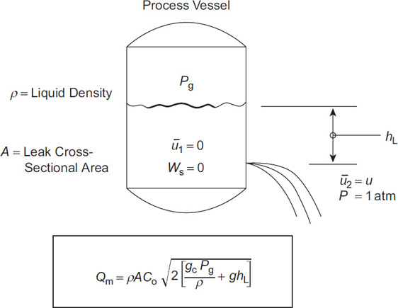
The gauge pressure on the tank is P_g, and the external gauge pressure is atmospheric, or 0. The shaft work W_s is zero, and the velocity of the fluid in the tank is zero.

A dimensionless discharge coefficient C₁ is defined as

$\begin{matrix} - \frac{Δ P}{ρ} - \frac{g}{g_{c}} Δ z - F = C_{1}^{2} (- \frac{Δ P}{ρ} - \frac{g}{g_{c}} Δ z) & (4-8) \end{matrix}$

The mechanical energy balance (Equation 4-1) is solved for ū, the average instantaneous discharge velocity from the leak:

$\begin{matrix} \bar{u} = C_{1} \sqrt{α} \sqrt{2 (\frac{g {}_{c}P_{g}^{}}{ρ} + g h_{L})} & (4-9) \end{matrix}$

where h_L is the liquid height above the leak. A new discharge coefficient C_o is defined as

$\begin{matrix} C_{o} = C_{1} \sqrt{α} & (4-10) \end{matrix}$

The resulting equation for the instantaneous velocity of fluid exiting the leak is

$\begin{matrix} \bar{u} = C_{o} \sqrt{2 (\frac{g {}_{c}P_{g}^{}}{ρ} + g h_{L})} & (4-11) \end{matrix}$

The instantaneous mass flow rate Q_m resulting from a hole of area A is given by

$\begin{matrix} \begin{matrix} Q_{m} = ρ \bar{u} A = ρ A C_{o} \sqrt{2 (\frac{g_{c} P_{g}}{ρ} + g h_{L})} \end{matrix} & (4-12) \end{matrix}$

As the tank empties, the liquid height decreases and the velocity and mass flow rate decrease.

Assume that the gauge pressure P_g on the surface of the liquid is constant. This would occur if the vessel was padded with an inert gas to prevent explosion or was vented to the atmosphere. For a tank of constant cross-sectional area A_t, the total mass of liquid in the tank above the leak is

$\begin{matrix} m = ρ A_{t} h_{L} & (4-13) \end{matrix}$

The rate of change of mass within the tank is

$\begin{matrix} \frac{d m}{d t} = - Q_{m} & (4-14) \end{matrix}$

where Q_m is given by Equation 4-12. By substituting Equations 4-12 and 4-13 into Equation 4-14, and by assuming a constant tank cross-section and liquid density, we can obtain a differential equation representing the change in the fluid height:

$\begin{matrix} \frac{d h_{L}}{d t} = - \frac{C_{o} A}{A_{t}} \sqrt{2 (\frac{g {}_{c}P_{g}^{}}{ρ} + g h_{L})} & (4-15) \end{matrix}$

Equation 4-15 can be rearranged and integrated from an initial height $h_{L}^{0}$ to any height h_L:

$\begin{matrix} \int_{h_{L}^{0}}^{h_{L}} \frac{d h_{L}}{\sqrt{\frac{2 g_{c} P_{g}}{ρ} + 2 g h_{L}}} = - \frac{C_{o} A}{A_{t}} \int_{0}^{t} d t & (4-16) \end{matrix}$

This equation is integrated to

$\begin{matrix} \frac{1}{g} \sqrt{\frac{2 g_{c} P_{g}}{ρ} + 2 g h_{L}} - \frac{1}{g} \sqrt{\frac{2 g_{c} P_{g}}{ρ} + 2 g h_{L}^{o}} = - \frac{C_{o} A}{A_{t}} t & (4-17) \end{matrix}$

Solving for h_L, the liquid level height in the tank, yields

$\begin{matrix} \begin{matrix} h_{L} = h_{L}^{o} - \frac{C_{o} A}{A_{t}} \sqrt{\frac{2 g {}_{c}P_{g}^{}}{ρ} + 2 g h_{L}^{o}} t + \frac{g}{2} {(\frac{C_{o} A}{A_{t}} t)}^{2} \end{matrix} & (4-18) \end{matrix}$

Equation 4-18 is substituted into Equation 4-12 to obtain the mass discharge rate at any time t:

$\begin{matrix} \begin{matrix} Q_{m} = ρ C_{o} A \sqrt{2 (\frac{g {}_{c}P_{g}^{}}{ρ} + g h_{L}^{o})} - \frac{ρ g C_{o}^{2} A^{2}}{A_{t}} t \end{matrix} & (4-19) \end{matrix}$

The first term on the right-hand side of Equation 4-19 is the initial mass discharge rate at $h_{L} = h_{L}^{o}$ .

The time t_e for the vessel to empty to the level of the leak is found by solving Equation 4-18 for t after setting h_L = 0:

$\begin{matrix} \begin{matrix} t_{e} = \frac{1}{C_{o} g} (\frac{A_{t}}{A}) [\sqrt{2 (\frac{g {}_{c}P_{g}^{}}{ρ} + g h_{L}^{o})} - \sqrt{\frac{2 g {}_{c}P_{g}^{}}{ρ}}] \end{matrix} & (4-20) \end{matrix}$

If the vessel is at atmospheric pressure, P_g = 0 and Equation 4-20 reduces to

$\begin{matrix} \begin{matrix} t_{e} = \frac{1}{C_{o} g} (\frac{A_{t}}{A}) \sqrt{2 g h_{L}^{o}} \end{matrix} & (4-21) \end{matrix}$

Example 4-2

A cylindrical tank 20 ft high and 8 ft in diameter is used to store benzene. The tank is padded with nitrogen to a constant regulated pressure of 1 atm gauge to prevent the formation of a flammable mixture. The liquid level within the tank is presently at 17 ft. A 1-in.-diameter puncture hole occurs in the tank 5 ft off the ground because of the careless driving of a forklift truck. Estimate (a) the gallons of benzene spilled, (b) the time required for the benzene to leak out, and (c) the maximum mass flow rate of benzene through the leak. The specific gravity of benzene at these conditions is 0.8794.

Solution

The density of the benzene is

$ρ = (0.8794) (62.4 {lb}_{m} / {ft}^{3}) = 54.9 {lb}_{m} / {ft}^{3}$

The area of the tank is

$A_{t} = \frac{π d^{2}}{4} = \frac{(3.14) {(8 ft)}^{2}}{4} = 50.2 {ft}^{2}$

The area of the leak is

$A = \frac{(3.14) {(1 in)}^{2} (1 {ft}^{2} / 144 {in}^{2})}{4} = 5.45 \times 10^{- 3} {ft}^{2}$

The gauge pressure is

$P_{g} = (1 atm) (14.7 {lb}_{f} / {in}^{2}) (144 {in}^{2} / {ft}^{2}) = 2.12 \times 10^{3} {lb}_{f} / {ft}^{2}$

The volume of benzene above the leak is

$V = A_{t} h_{L}^{0} = (50.2 {ft}^{2}) (17 ft - 5 ft) (7.48 {gal/ft}^{3}) = 4506 gal$

This is the total amount of benzene that will leak out.
The length of time for the benzene to leak out is given by Equation 4-20:

$\begin{matrix} \end{matrix} \begin{matrix} t_{e} & = \frac{1}{C_{o} g} (\frac{A_{t}}{A}) [\sqrt{2 (\frac{g_{c} P_{g}}{ρ} + g h_{L}^{o})} - \sqrt{\frac{2 g_{c} P_{g}}{ρ}}] \\ = \frac{1}{(0.61) (32.17 {ft/s}^{2})} (\frac{50.2 {ft}^{2}}{5.45 \times 10^{- 3} {ft}^{2}}) \\ \times {[\frac{(2) (32.17 {ft-lb}_{m} {/lb}_{f} {-s}^{2})}{54.9 {lb}_{m} {/ft}^{3}} \\ {+ (2) (32.17 {ft/s}^{2}) (12 ft)]}^{1 / 2} - \sqrt{2484 {ft}^{2} {/s}^{2}}} \\ = (469 s^{2} /ft) (7.22 ft/s) = 3386 s = 56.4 min \end{matrix}$

This appears to be more than adequate time to stop the leak or to invoke an emergency procedure to reduce the impact of the leak. However, the maximum discharge occurs when the hole first occurs.
The maximum discharge occurs at t = 0 at a liquid level of 17.0 ft. Equation 4-19 is used with t = 0 to compute the mass flow rate:

$\begin{matrix} Q_{m} & = ρ A C_{o} \sqrt{2 (\frac{g_{c} P_{g}}{ρ} + g h_{L}^{o})} \\ = (54.9 1 b_{m} / {ft}^{3}) (5.45 \times 10^{- 3} {ft}^{2}) (0.61) \sqrt{3.26 \times 10^{3} {ft}^{2} / s^{2}} \\ = 10.4 1 b_{m} / s \end{matrix}$

A general equation to represent the draining time for any vessel of any geometry is developed as follows. Assume that the head space above the liquid is at atmospheric pressure. Then, by combining Equations 4-12 and 4-14, we get

$\begin{matrix} \frac{d m}{d t} = ρ \frac{d V}{d t} = - ρ A C_{o} \sqrt{2 g h_{L}} & (4-22) \end{matrix}$

By rearranging and integrating, we obtain

$\begin{matrix} \begin{matrix} - \frac{1}{A C_{o} \sqrt{2 g}} \int_{v_{1}}^{v_{2}} \frac{d V}{\sqrt{h_{L}}} = \int_{0}^{t} d t \end{matrix} & (\begin{matrix} 4-23 \end{matrix}) \end{matrix}$

which results in the general equation for the draining time for any vessel:

$\begin{matrix} \begin{matrix} t = \frac{1}{A C_{o} \sqrt{2 g}} \int_{V_{1}}^{V_{2}} \frac{d V}{\sqrt{h_{L}}} \end{matrix} & (4-24) \end{matrix}$

Equation 4-24 does not assume that the hole is at the bottom of the vessel.

For a vessel with the shape of a vertical cylinder, we have

$\begin{matrix} d V = \frac{π d^{2}}{4} d h_{L} & (4-25) \end{matrix}$

By substituting into Equation 4-24, we obtain

$\begin{matrix} t = \frac{π D^{2}}{4 A C_{o} \sqrt{2 g}} \int \frac{d h_{L}}{\sqrt{h_{L}}} & (4-26) \end{matrix}$

If the hole is at the bottom of the vessel, then Equation 4-26 is integrated from h = 0 to $h = h_{L}^{0}$ .

Equation 4-26 then provides the emptying time for the vessel:

$\begin{matrix} t_{e} = \frac{π D^{2} / 4}{A C_{o}} \sqrt{\frac{2 h_{L}^{o}}{g}} = \frac{1}{C_{o} g} (\frac{π D^{2} / 4}{A}) \sqrt{2 g h_{L}^{0}} & (4-27) \end{matrix}$

which is the same result as Equation 4-21.

4-4 Flow of Liquids through Pipes

A pipe transporting liquid is shown in Figure 4-6. A pressure gradient across the pipe is the driving force for the movement of liquid. If the pipe diameter is constant, then the velocity is constant along the entire length of the pipe. Frictional forces between the liquid and the wall of the pipe convert kinetic energy into thermal energy, which in turn results in a decrease in the liquid pressure.

A figure shows the liquid flow through a constant-diameter pipe. — **Figure 4-6** Liquid flowing through a constant-diameter pipe. The frictional flow losses between the fluid and the pipe wall result in a pressure drop across the pipe length. Kinetic energy changes are usually negligible because the velocity is constant.

A figure illustrates the flow of a liquid through a constant-diameter pipe. P subscript 1, u overbar subscript 1, and Z subscript 1, are the parameters of the fluid entering the pipe. P 2, u overbar subscript 2, and Z 2, represents the parameters of the fluid leaving the pipe. P2 is less than P1, and u overbar subscript 2, equals u overbar subscript 1. The length of the pipe is L, and the liquid density, rho is constant.

Flow of incompressible liquids through pipes is described by the mechanical energy balance (Equation 4-1) combined with the incompressible fluid assumption (Equation 4-2). The net result is

$\begin{matrix} \frac{Δ P}{ρ} + \frac{Δ {\bar{u}}^{2}}{2 α g_{c}} + \frac{g}{g_{c}} Δ z + F = - \frac{W_{s}}{m} & (4-28) \end{matrix}$

The frictional loss term F in Equation 4-28 represents the loss of mechanical energy resulting from friction. It includes losses resulting from flow through lengths of pipe; fittings such as valves, elbows, orifices; and pipe entrances and exits. For each frictional device, a loss term of the following form is used:

$\begin{matrix} F = K_{f} (\frac{u^{2}}{2 g_{c}}) & (4-29) \end{matrix}$

where

K_f is the excess head loss due to the pipe or pipe fitting (dimensionless) and u is the fluid velocity (length/time).

For fluids flowing through pipes, the excess head loss term K_f is given by

$\begin{matrix} K_{f} = \frac{4 f L}{d} & (4-30) \end{matrix}$

where

f is the Fanning friction factor (unitless),

L is the flow path length (length), and

d is the flow path diameter (length).

The Fanning friction factor f is a function of the Reynolds number Re and the roughness of the pipe ε. Table 4-1 provides values of ε for various types of clean pipe. Figure 4-7 is a plot of the Fanning friction factor versus Reynolds number with the pipe roughness, ε/d, as a parameter.

A plot of Fanning friction factor, f, against Reynolds number is illustrated. — **Figure 4-7** Plot of Fanning friction factor f versus Reynolds number. (Source: Octave Levenspiel. *Engineering Flow and Heat Exchange* (New York, NY: Plenum Press, 1984), p. 20.)

A graph of fanning friction factor, f, versus Reynolds number is shown. The horizontal axis represents Reynolds number, and ranges from 10 to the power 2, to 10 to the power 8. The left vertical axis represents the Fanning friction factor, f, and ranges from 0.002 to 0.025. The right vertical axis represents the relative roughness, epsilon over d, and ranges from 0.0001 to 0.05. The linear curve representing the laminar flow is steeply decreasing. It ranges between 0.025 and 0.075 of fanning friction factor, and around 10 cubed of Reynolds number. The curves representing the relative roughness, start between the range of 0.012 to 0.055, and end between the range of 0.001 to 0.05. The smooth pipe curve has an epsilon value of 0. The relative roughness curves range between 10,500 and 10 to the power 8, of the Reynolds number.

Table 4-1 Roughness Factor ε for Pipes^a

Pipe material	Condition	Typical ε
Pipe material	Condition	mm	inch
Drawn brass, copper, stainless	New	0.002	0.00008
Commercial steel	New	0.046	0.0018
	Light rust	0.3	0.015
	General rust	2.0	0.08
Iron	Wrought, new	0.045	0.0018
	Cast, new	0.30	0.025
	Galvanized	0.15	0.006
Concrete	Very smooth	0.04	0.0016
	Wood floated, brushed	0.3	0.012
	Rough, visible form marks	2.0	0.08
Glass or plastic	Drawn tubing	0.002^c	0.0008^c
Rubber	Smooth tubing	0.01	0.004
	Wire reinforced	1.0	0.04
Fiberglass^b		0.005	0.0002

^aRon Darby. “Fluid Flow.” Albright’s Chemical Engineering Handbook, Lyle F. Albright, ed. (Boca Raton, FL: CRC Press, 2009), p. 421.

^bWilliam D. Stringfellow, ed. Fiberglass Pipe Handbook (Washington, DC: Society of the Plastics Industry, 1989).

^cGenerally considered smooth pipe with ε = 0.

For laminar flow, the Fanning friction factor is given by

$\begin{matrix} f = \frac{16}{R e} & (4-31) \end{matrix}$

For turbulent flow, the data shown in Figure 4-7 are represented by the Colebrook equation:

$\begin{matrix} \frac{1}{\sqrt{f}} = - 4 \log (\frac{1}{3.7} \frac{ε}{d} + \frac{1.255}{R e \sqrt{f}}) & (4-32) \end{matrix}$

An alternative form of Equation 4-32, useful for determining the Reynolds number from the friction factor f, is

$\begin{matrix} \frac{1}{R e} = \frac{\sqrt{f}}{1.255} (10^{- 0.25/ \sqrt{f}} - \frac{1}{3.7} \frac{ε}{d}) & (4-33) \end{matrix}$

For fully developed turbulent flow in rough pipes, f is independent of the Reynolds number, as shown by the nearly constant friction factors at high Reynolds numbers in Figure 4-7. For this case, Equation 4-33 is simplified to

$\begin{matrix} \frac{1}{\sqrt{f}} = 4 \log (3.7 \frac{d}{ε}) & (4-34) \end{matrix}$

For smooth pipes, ε = 0 and Equation 4-32 reduces to

$\begin{matrix} \frac{1}{\sqrt{f}} = 4 \log (\frac{Re \sqrt{f}}{1.255}) & (4-35) \end{matrix}$

For smooth pipes with a Reynolds number less than 100,000, the following Blasius approximation to Equation 4-35 is useful:

$\begin{matrix} f = 0.079 R e^{- 1 / 4} & (4-36) \end{matrix}$

A single equation has been proposed by Chen³ to provide the friction factor f over the entire range of Reynolds numbers shown in Figure 4-7. This equation is

³N. H. Chen. An Explicit Equation for Friction Factor in Pipe, Industrial Engineering and Chemistry Fundamentals 18 (1979): 296.

$\begin{matrix} \frac{1}{\sqrt{f}} = - 4 \log (\frac{ε / d}{3.7065} - \frac{5.0452 \log A}{R e}) & (4-37) \end{matrix}$

where

$A = [\frac{{(ε / d)}^{1.1098}}{2.8257} + \frac{5.8506}{R e^{0.8981}}]$

2-K Method

For pipe fittings, valves, and other flow obstructions, the traditional method has been to use an equivalent pipe length L_equiv in Equation 4-30. The problem with this method is that the specified length is coupled to the friction factor. An improved approach is to use the 2-K method,⁴, ⁵ which uses the actual flow path length in Equation 4-30—equivalent lengths are not used—and provides a more detailed approach for pipe fittings, inlets, and outlets. Darby⁶ suggests a 3-K method that fits the data over an even wider range of flow conditions.

⁴W. B. Hooper. The Two-K Method Predicts Head Losses in Pipe Fittings, Chemical Engineering (August 24, 1981): 96–100.

⁵W. B. Hooper. Calculate Head Loss Caused by Change in Pipe Size, Chemical Engineering (November 7, 1988): 89–92.

⁶R. Darby and R. P. Chhabra. Chemical Engineering Fluid Mechanics, 3rd ed. (Boca Raton, FL: CRC Press, 2017).

The 2-K method defines the excess head loss in terms of two constants, the Reynolds number and the pipe internal diameter:

$\begin{matrix} K_{f} = \frac{K_{1}}{R e} + K_{\infty} (1+ \frac{1}{I D_{inches}}) & (4-38) \end{matrix}$

where

K_f is the excess head loss (dimensionless),

K_l and K_∞ are constants (dimensionless),

Re is the Reynolds number (dimensionless), and

ID_inches is the internal diameter of the flow path (inches).

Table 4-2 contains a list of K values for use in Equation 4-38 for various types of fittings and valves.

Table 4-2 2-K Constants for Loss Coefficients in Fittings and Valves

Fittings	Description of fitting	K₁	K_∞
Elbows	Standard (r/D = 1), threaded	800	0.40
90°	Standard (r/D = 1), flanged/welded	800	0.25
	Long radius (r/D = 1.5), all types	800	0.20
	Mitered (r/D = 1.5): 1 weld (90°)	1000	1.15
	2 welds (45°)	800	0.35
	3 welds (30°)	800	0.30
	4 welds (22.5°)	800	0.27
	5 welds (18°)	800	0.25
45°	Standard (r/D = 1), all types	500	0.20
	Long radius (r/D = 1.5)	500	0.15
	Mitered, 1 weld (45°)	500	0.25
	Mitered, 2 welds (22.5°)	500	0.15
180°	Standard (r/D = 1), threaded	1000	0.60
	Standard (r/D = 1), flanged/welded	1000	0.35
	Long radius (r/D = 1.5), all types	1000	0.30
Tees
Used as elbows	Standard, threaded	500	0.70
	Long radius, threaded	800	0.40
	Standard, flanged/welded	800	0.80
	Stub-in branch	1000	1.00
Run-through	Threaded	200	0.10
	Flanged/welded	150	0.50
	Stub-in branch	100	0.00
Valves
Gate, ball or plug	Full line size, β = 1.0	300	0.10
	Reduced trim,β = 0.9	500	0.15
	Reduced trim,β = 0.8	1000	0.25
Globe	Standard	1500	4.00
	Angle or Y-type	1000	2.00
Diaphragm	Dam type	1000	2.00
Butterfly		800	0.25
Check	Lift	2000	10.0
	Swing	1500	1.50
	Tilting disk	1000	0.50

Source: William B. Hooper. The Two-K Method Predicts Head Losses in Pipe Fittings, Chemical Engineering (August 24, 1981): 97.

For pipe entrances and exits, Equation 4-38 is modified to account for the change in kinetic energy:

$\begin{matrix} K_{f} = \frac{K_{1}}{R e} + K_{\infty} & (4-39) \end{matrix}$

For pipe entrances, K₁ = 160 and K_∞ = 0.50 for a normal entrance. For a Borda-type pipe connection to a tank where the pipe sticks up into the bottom of the tank for a short distance, K_∞ = 1.0. For pipe exits, K₁ = 0 and K_∞ = 1.0. The K factors for the entrance and exit effects account for the changes in kinetic energy through these piping changes, so no additional kinetic energy terms in the mechanical energy balance must be considered. For high Reynolds numbers (that is, Re > 10,000), the first term in Equation 4-39 is negligible and K_f = K_∞. For low Reynolds numbers (that is, Re < 50), the first term dominates and K_f = K₁/Re.

Equations are also available for orifices⁷ and for changes in pipe sizes.⁸

⁷W. B. Hooper. The Two-K Method Predicts Head Losses in Pipe Fittings, Chemical Engineering (August 24, 1981): 96–100.

⁸W. B. Hooper. Calculate Head Loss Caused by Change in Pipe Size, Chemical Engineering (November 7, 1988): 89–92.

The 2-K method also represents liquid discharge through holes. From the 2-K method, an expression for the discharge coefficient for liquid discharge through a hole can be determined. The result is

$\begin{matrix} C_{o} = \frac{1}{\sqrt{1 + \sum K_{f}}} & (4-40) \end{matrix}$

where $\sum K_{f}$ is the sum of all excess head loss terms, including entrances, exits, pipe lengths, and fittings, provided by Equations 4-30, 4-38, and 4-39. For a simple hole in a tank with no pipe connections or fittings, the friction is caused only by the entrance and exit effects of the hole. For Reynolds numbers greater than 10,000, K_f = 0.5 for the entrance and K_f = 1.0 for the exit. Thus ∑ K_f = 1.5, and from Equation 4-40, C_o = 0.63, which nearly matches the suggested value of 0.61.

The general solution procedure to determine the mass flow rate of discharged material from a piping system is as follows:

Given the length, diameter, and type of pipe; pressures and elevation changes across the piping system; work input or output to the fluid resulting from pumps, turbines, and other sources; the number and type of fittings in the pipe; and properties of the fluid, including density and viscosity.
Specify the initial point (point 1) and the final point (point 2). This must be done carefully, because the individual terms in Equation 4-28 are highly dependent on this specification.
Determine the pressures and elevations at points 1 and 2. Determine the initial fluid velocity at point 1.
Guess a value for the velocity at point 2. If fully developed turbulent flow is expected, then this is not required.
Determine the friction factor for the pipe using Equations 4-31 through 4-37.
Determine the excess head loss terms for the pipe (using Equation 4-30), for the fittings (using Equation 4-38), and for any entrance and exit effects (using Equation 4-39). Sum the head loss terms, and compute the net frictional loss term using Equation 4-29. Use the velocity at point 2.
Compute values for all the terms in Equation 4-28, and substitute into the equation. If the sum of all the terms in Equation 4-28 is zero, then the computation is completed. If not, go back to step 4 and repeat the calculation.
Determine the mass flow rate using the equation $\dot{m} = ρ \bar{u} A .$ .

If fully developed turbulent flow is expected, the solution is direct. Substitute the known terms into Equation 4-28, leaving the velocity at point 2 as a variable. Solve for the velocity directly.

Example 4-3

Water contaminated with small amounts of hazardous waste is gravity-drained out of a large storage tank through a straight, new commercial steel pipe, 100 mm ID (actual internal diameter). The pipe is 100 m long, with a gate valve near the tank. The entire pipe assembly is horizontal. If the liquid level in the tank is 5.8 m above the pipe outlet, and the pipe is severed 33 m from the tank, compute the flow rate of material escaping from the pipe.

Solution

The draining operation is shown in Figure 4-8. Assuming negligible kinetic energy changes, no pressure changes, and no shaft work, the mechanical energy balance (Equation 4-28) applied between points 1 and 2 reduces to

Draining operation is represented in a figure. — **Figure 4-8** Draining geometry for Example 4-3.

A figure illustrates a draining geometry. The liquid from the tank is discharged via a gate valve. The liquid level in the tank is at a height of 5.8 meter above the level of the pipe. The pipe is a 100 millimeter I D commercial steel pipe. The length of the pipe including the gate valve is 33 meters. The liquid inside the tank is labeled, 1, and the liquid discharged is labeled, 2.

$\frac{g}{g_{c}} Δ z + F = 0$

For water,

$\begin{matrix} \begin{matrix} μ \end{matrix} & = 1.0 \times 10^{- 3} kg/m s \\ ρ & = 1000 {kg/m}^{3} \end{matrix}$

The K factors for the entrance and exit effects are determined using Equation 4-39. The K factor for the gate valve is found in Table 4-2, and the K factor for the pipe length is given by Equation 4-30.

For the pipe entrance,

$K_{f} = \frac{160}{R e} + 0.50$

For the gate valve,

$K_{f} = \frac{300}{R e} + 0.10$

For the pipe exit,

$K_{f} = 1.0$

For the pipe length,

$K_{f} = \frac{4 f L}{d} = \frac{4 f (33 m)}{0.10 m} = 1320 f$

Summing the K factors gives

$\sum K_{f} = \frac{460}{Re} + 1320 f + 1.60$

For Re > 10,000, the first term in the equation is small. Thus

$\sum K_{f} = 1320 f + 1.60$

and it follows that

$F = \sum K_{f} (\frac{{\bar{u}}^{2}}{2 g_{c}}) = (660 f + 0.80) (\frac{{\bar{u}}^{2}}{g_{c}})$

The gravitational term in the mechanical energy equation is given by

$\frac{g}{g_{c}} Δ z = \frac{9.8 {m/s}^{2}}{1 kg {m/s}^{2} / N} (0-5.8 m) = - 56.8 Nm/kg = - 56.8 J/kg$

Because there is no pressure change and no pump or shaft work, the mechanical energy balance (Equation 4-28) reduces to

$\frac{{\bar{u}}_{2}^{2}}{2 g_{c}} + \frac{g}{g_{c}} Δ z + F = 0 .$

Solving for the exit velocity and substituting for the height change gives

${\bar{u}}_{2}^{2} = - 2 g_{c} (\frac{g}{g_{c}} Δ z + F) = - 2 g_{c} (- 56.8 + F)$

The Reynolds number is given by

$R e = \frac{d \bar{u} ρ}{μ} = \frac{(0.1 m) (\bar{u}) (1000 {kg/m}^{3})}{1.0 \times 10^{- 3} kg/m s} = 1.0 \times 10^{5} \bar{u}$

For new commercial steel pipe, from Table 4-1, ε = 0.046 mm and

$\frac{ε}{d} = \frac{0.046 mm}{100 mm} = 0.00046$

Because the friction factor f and the frictional loss term F are functions of the Reynolds number and velocity, the solution is found by trial and error. The trial-and-error solution is shown in the following table:

Guessed ū (m/s)	Re	f	F	Calculated ū (m/s)
3.00	300,000	0.00451	34.09	6.75
3.50	350,000	0.00446	46.00	4.66
3.66	366,000	0.00444	50.18	3.66

Thus, the velocity of the liquid discharging from the pipe is 3.66 m/s. The table also shows that the friction factor f changes little with the Reynolds number. Thus, we can approximate it using Equation 4-34 for fully developed turbulent flow in rough pipes. Equation 4-34 produces a friction factor value of 0.0041. Then

$F = (660 f + 0.80) {\bar{u}}_{2}^{2} = 3.51 {\bar{u}}_{2}^{2}$

By substituting and solving, we obtain

$\begin{matrix} {\bar{u}}_{2}^{2} & = - 2 g_{c} (- 56.8 + 3.51 {\bar{u}}_{2}^{2}) \\ = 113.6 - 7.02 {\bar{u}}_{2}^{2} \\ {\bar{u}}_{2} & = 3.76 m/s \end{matrix}$

This result is close to the more exact trial-and-error solution.

The cross-sectional area of the pipe is

$A = \frac{π d^{2}}{4} = \frac{(3.14) (0.1 m^{2})}{4} = 0.00785 m^{2}$

The mass flow rate is given by

$Q_{m} = ρ \bar{u} A = (1000 {kg/m}^{3}) (3.66 m/s) (0.00785 m^{2}) = 28.8 kg/s$

This represents a significant flow rate. If the plant personnel are able to recognize the leak and respond in 15 min to stop the release, a total of 26,000 kg of hazardous waste will be spilled. In addition to the material released by the flow, the liquid contained within the pipe between the valve and the rupture will spill. An alternative system must be designed to limit the release. This could include a reduction in the emergency response period, replacement of the pipe by a pipe with a smaller diameter, or modification of the piping system to include additional remotely activated control valves to stop the flow.

4-5 Flow of Gases or Vapors through Holes

For flowing liquids, the kinetic energy changes are frequently negligible and the physical properties (particularly the density) are constant. For flowing gases and vapors, these assumptions are valid only for small pressure changes (P₁/P₂ < 2) and low velocities (less than 0.3 times the speed of sound in gas). Energy contained within the gas or vapor as a result of its pressure is converted into kinetic energy as the gas or vapor escapes and expands through the hole. The density, pressure, and temperature change as the gas or vapor exits through the leak.

Gas and vapor discharges are classified as either throttling or free expansion releases. In throttling releases, the gas issues through a small crack with large frictional losses; little of the energy inherent to the gas pressure is converted to kinetic energy. In free expansion releases, most of the pressure energy is converted to kinetic energy, so that the assumption of isentropic behavior is usually valid.

Source models for throttling releases require detailed information on the physical structure of the leak; they are not considered here. Free expansion release source models require only the diameter of the leak.

A free expansion leak is shown in Figure 4-9. The mechanical energy balance (Equation 4-1) describes the flow of compressible gases and vapors. Assuming negligible potential energy changes and no shaft work results in a reduced form of the mechanical energy balance describing compressible flow through holes:

Expansion of the gas through a hole in a process unit is illustrated in a figure. — **Figure 4-9** A free expansion gas leak. The gas expands isentropically through the hole. The gas properties (P, T) and velocity change during the expansion.

A figure shows the expansion of gas through a hole in a process unit. Variables representing the gas pressurized within the process unit are, P 0, T 0, u overbar subscript 0, equals 0, delta z equals 0, and W subscript s, equals 0. The gas escapes into the external surroundings via a hole. The variables at the throat are, P and u overbar less than Sonic velocity.

$\begin{matrix} \int \frac{d P}{ρ} + Δ (\frac{{\bar{u}}^{2}}{2 α g_{c}}) + F = 0 & (4-41) \end{matrix}$

A discharge coefficient C_l is defined in a similar fashion to the coefficient defined in Section 4-2:

$\begin{matrix} - \int \frac{d P}{ρ} - F = C_{1}^{2} (- \int \frac{d P}{ρ}) & (4-42) \end{matrix}$

Equation 4-42 is combined with Equation 4-41 and integrated between any two convenient points. An initial point (denoted by subscript “o”) is selected where the velocity is zero and the pressure is P_o. The integration is completed to any arbitrary final point (denoted without a subscript). The result is

$\begin{matrix} C_{1}^{2} \int_{P_{o}}^{P} \frac{d P}{ρ} + \frac{{\bar{u}}^{2}}{2 α g_{c}} = 0 & (4-43) \end{matrix}$

For any ideal gas undergoing an isentropic expansion,

$\begin{matrix} P v^{γ} = \frac{P}{ρ^{γ}} = constant & (4-44) \end{matrix}$

where γ is the ratio of the heat capacities, γ = C_p/C_v. Substituting Equation 4-44 into Equation 4-43, defining a new discharge coefficient C_o identical to that in Equation 4-5, and integrating results in an equation representing the velocity of the fluid at any point during the isentropic expansion:

$\begin{matrix} {\bar{u}}^{2} = 2 g_{c} C_{o}^{2} \frac{γ}{γ - 1} \frac{P_{o}}{ρ_{0}} [1 - {(\frac{P}{P_{o}})}^{(γ - 1) / γ}] = \frac{2 g_{c} C_{o}^{2} R_{g} T_{o}}{M} \frac{γ}{γ - 1} [1 - {(\frac{P}{P_{o}})}^{(γ - 1) / γ}] & (4-45) \end{matrix}$

The second form incorporates the ideal gas law for the initial density ρ_o. R_g is the ideal gas constant, and T_o is the temperature of the source. Using the continuity equation

$\begin{matrix} Q_{m} = ρ \bar{u} A & (4-46) \end{matrix}$

and the ideal gas law for isentropic expansions in the form

$\begin{matrix} ρ = ρ_{o} {(\frac{P}{P_{o}})}^{1 / γ} & (4-47) \end{matrix}$

results in the following expression for the mass flow rate:

$\begin{matrix} \begin{matrix} Q_{m} = C_{o} A P_{o} \sqrt{\frac{2 g_{c} M}{R_{g} T_{o}} \frac{γ}{γ - 1} [{(\frac{P}{P_{o}})}^{2 / γ} - {(\frac{P}{P_{o}})}^{(γ + 1) / γ}]} \end{matrix} & (4-48) \end{matrix}$

Equation 4-48 describes the mass flow rate at any point during the isentropic expansion.

For many safety studies, the maximum flow rate of vapor through the hole is required. This is determined by differentiating Equation 4-48 with respect to P/P_o and setting the derivative equal to zero. The result is solved for the pressure ratio resulting in the maximum flow:

$\begin{matrix} \begin{matrix} \frac{P_{choked}}{P_{o}} = {(\frac{2}{γ + 1})}^{γ / (γ - 1)} \end{matrix} & (4-49) \end{matrix}$

The choked pressure P_choked is the maximum downstream pressure resulting in maximum flow through the hole or pipe. For downstream pressures less than P_choked, the following statements are valid: (1) The velocity of the fluid at the throat of the leak is the velocity of sound at the prevailing conditions, and (2) the velocity and mass flow rate cannot be increased further by reducing the downstream pressure—they are independent of the downstream conditions. This type of flow is called choked, critical, or sonic flow and is illustrated in Figure 4-10.

Choked flow of gas through a hole is represented in a figure. — **Figure 4-10** Choked flow of gas through a hole. The gas velocity is sonic at the throat. The mass flow rate is independent of the downstream pressure.

A figure shows the choked flow of gas through a hole. The pressurized gas within the process unit is represented with the following variables, P 0, T 0, and u overbar 0, equals 0. The pressure of the gas at the throat is P, which equals P subscript choked. The sonic velocity at the throat equals u overbar. The pressure of the gas in the external surroundings is P, which is less than P subscript choked.

An interesting feature of Equation 4-49 is that for ideal gases, the choked pressure is a function only of the heat capacity ratio γ. Thus:

Gas	γ	P_choked
Monatomic	≅ 1.67	0.487P_o
Diatomic and air	≅ 1.40	0.528P_o
Triatomic	≅ 1.32	0.542P_o

For an air leak to atmospheric conditions (P_choked = 14.7 psia), if the upstream pressure is greater than 14.7/0.528 = 27.8 psia, or 13.1 psig, the flow will be choked and maximized through the leak. Conditions leading to choked flow are common in the process industries.

The maximum flow is determined by substituting Equation 4-49 into Equation 4-48:

$\begin{matrix} \begin{matrix} {(Q_{m})}_{choked} = C_{o} A P_{o} \sqrt{\frac{γ g_{c} M}{R_{g} T_{o}} {(\frac{2}{γ + 1})}^{(γ + 1) / (γ - 1)}} \end{matrix} & (4-50) \end{matrix}$

where

M is the molecular weight of the escaping vapor or gas,

T_o is the temperature of the source, and

R_g is the ideal gas constant.

For sharp-edged orifices with Reynolds numbers greater than 30,000 (and not choked), a constant discharge coefficient C_o of 0.61 is indicated. However, for choked flows the discharge coefficient increases as the downstream pressure decreases.⁹ For these flows and for situations where C_o is uncertain, a conservative value of 1.0 is recommended.

⁹Robert H. Perry and Cecil H. Chilton. Chemical Engineers Handbook, 7th ed. (New York, NY: McGraw-Hill, 1997), pp. 10–16.

Values for the heat capacity ratio γ for a variety of gases are provided in Table 4-3.

Table 4-3 Heat Capacity Ratios γ for Selected Gases

Gas	Chemical formula or symbol	Approximate molecular weight (M)	Heat capacity ratio γ = C_p/C_v
Acetylene	C₂H₂	26.0	1.30
Air	–	29.0	1.40
Ammonia	NH₃	17.0	1.32
Argon	Ar	39.9	1.67
Butane	C₄H₁₀	58.1	1.11
Carbon dioxide	CO₂	44.0	1.30
Carbon monoxide	CO	28.0	1.40
Chlorine	Cl₂	70.9	1.33
Ethane	C₂H₆	30.0	1.22
Ethylene	C₂H₄	28.0	1.22
Helium	He	4.0	1.66
Hydrogen	H₂	2.0	1.41
Hydrogen chloride	HCl	36.5	1.41
Hydrogen sulfide	H₂S	34.1	1.30
Methane	CH₄	16.0	1.32
Methyl chloride	CH₃Cl	50.5	1.20
Natural gas	–	19.5	1.27
Nitric oxide	NO	30.0	1.40
Nitrogen	N₂	28.0	1.41
Nitrous oxide	N₂O	44.0	1.31
Oxygen	O₂	32.0	1.40
Propane	C₃H₈	44.1	1.15
Propene (propylene)	C₃H₆	42.1	1.14
Sulfur dioxide	SO₂	64.1	1.26

Source: Crane Co. Flow of Fluids through Valves, Fittings, and Pipes, Technical Paper 410 (New York, NY: Crane Co., 2009). www.flowoffluids.com.

Example 4-4

A 0.2-cm hole forms in a tank containing nitrogen at 14 bar gauge and 25°C. Determine the mass flow rate through this leak. The external pressure is 1 atm.

Solution

From Table 4-3, for nitrogen γ = 1.41. Then, from Equation 4-49,

$\frac{P_{choked}}{P_{o}} = {(\frac{2}{γ + 1})}^{γ / (γ - 1)} = {(\frac{2}{2.41})}^{1.41 / 0.41} = 0.527$

The absolute pressure in the tank is 14 bar + 1.013 barg = 15.01 bara.

Thus,

$P_{choked} = 0.527 (15.01 bara) = 7.91 bara$

Any external pressure less than 7.91 bara will result in choked flow through the leak. Because the external pressure is atmospheric in this case (1.013 bara), choked flow is expected and Equation 4-50 applies. The area of the hole is

$A = \frac{π d^{2}}{4} = \frac{(3.14) {(0.2 cm)}^{2} (1 m^{2} / 10^{4} {cm}^{2})}{4} = 3.14 \times 10^{- 6} m^{2}$

The discharge coefficient C₀ is assumed to be 1.0. Also,

$\begin{matrix} T_{o} = 25 + 273 = 298 K \\ {(\frac{2}{γ + 1})}^{(γ + 1) / (γ - 1)} = {(\frac{2}{2.41})}^{2.41 / 0.41} = {0.830}^{5.87} = 0.335 \end{matrix}$

Then, using Equation 4-50,

$\begin{matrix} {\begin{matrix} (Q_{m}) \end{matrix}}_{choked} & = C_{o} {A P}_{o} \sqrt{{\frac{γ g_{c} M}{R_{g} T_{o}} (\frac{2}{γ + 1})}^{(γ + 1) (γ - 1)}} \\ = (1.0) (3.14 \times 10^{- 6} m^{2}) (15.01 bara) (\frac{10^{5} {N / m}^{2}}{1 bar}) \\ \times \sqrt{\frac{(1.41) (1 \frac{{kg m/s}^{2}}{N}) (28 kg/kg-mole)}{(8.314 \times 10^{3} N m/kg-mole K) (298 K)} (0.335)} \\ = 4.71 N \sqrt{5.34 \times 10^{- 6} {kg}^{2} / N^{2} S^{2}} \\ {\begin{matrix} (Q_{m}) \end{matrix}}_{choked} & = 1.09 \times 10^{- 2} kg/s \end{matrix}$

4-6 Flow of Gases or Vapors through Pipes

Gas flow through pipes is modeled using two special cases: adiabatic and isothermal behavior. The adiabatic case corresponds to rapid gas flow through an insulated pipe. The isothermal case corresponds to flow through an uninsulated pipe maintained at a constant temperature; an underwater pipeline is an example. Real vapor flows behave somewhere between the adiabatic and isothermal cases. Unfortunately, the real case must be modeled numerically and no generalized and useful equations are available.

For both the isothermal and adiabatic cases, it is convenient to define a dimensionless Mach (Ma) number as the ratio of the gas velocity to the velocity of sound in the gas at the prevailing conditions:

$\begin{matrix} Ma = \frac{\bar{u}}{a} & (4-51) \end{matrix}$

where a is the velocity of sound. The velocity of sound is determined using the thermodynamic relationship

$\begin{matrix} a = \sqrt{g_{c} {(\frac{\partial P}{\partial ρ})}_{S}} & (4-52) \end{matrix}$

which for an ideal gas is equivalent to

$\begin{matrix} a = \sqrt{γ g_{c} R_{g} T / M} & (\begin{matrix} 4-53 \end{matrix}) \end{matrix}$

This demonstrates that for ideal gases, the sonic velocity is a function of temperature only. For air at 20°C, the velocity of sound is 344 m/s (1129 ft/s).

Adiabatic Flows

An adiabatic pipe containing a flowing gas is shown in Figure 4-11. For this particular case, the outlet velocity is less than the sonic velocity. The flow is driven by a pressure gradient across the pipe. As the gas flows through the pipe, it expands because of a decrease in pressure. This expansion leads to an increase in velocity and an increase in the kinetic energy of the gas. The kinetic energy is extracted from the thermal energy of the gas; thus, a decrease in temperature occurs. However, frictional forces are present between the gas and the pipe wall. These frictional forces increase the temperature of the gas. Depending on the magnitude of the kinetic and frictional energy terms, either an increase or a decrease in the gas temperature is possible.

Adiabatic nonchoked flow of gas through a pipe is represented in a figure. — **Figure 4-11** Adiabatic nonchoked flow of gas through a pipe. The gas temperature might increase or decrease, depending on the magnitude of the frictional losses.

A figure illustrates the adiabatic nonchoked flow of gas through a pipe. Various parameters representing the gas entering into the pipe are, P1, T1, u overbar 1, and M times a 1. Q equals 0. The length of the pipe is, L. Various parameters representing the gas leaving the pipe are, P2 less than P1, P2 greater than P subscript choked, T2, u overbar 2 less than u overbar 1, u overbar 2, less than sonic velocity, Ma 2 less than Ma 1, and Ma 2 less than 1. For the surroundings, P equals P 2 which is less than P subscript choked.

The mechanical energy balance (Equation 4-1) also applies to adiabatic flows. For this case, it is more conveniently written in the form

$\begin{matrix} \frac{d P}{ρ} + \frac{\bar{u} d \bar{u}}{{α g}_{c}} + \frac{g}{g_{c}} d z + d F = - \frac{δ W_{s}}{m} & (4-54) \end{matrix}$

The following assumptions are valid for this case:

$\frac{g}{g_{c}} d z \approx 0$

Assuming a straight pipe without any valves or fittings, Equations 4-29 and 4-30 can be combined and then differentiated to result in

$d F = \frac{2 f {\bar{u}}^{2} d L}{g_{c} d}$

Because no mechanical linkages are present,

$δ W_{S} = 0$

An important part of the frictional loss term is the assumption of a constant Fanning friction factor f across the length of the pipe. This assumption is valid only at high Reynolds numbers.

A total energy balance is useful for describing the temperature changes within the flowing gas. For this open steady-flow process, the total energy balance is given by

$\begin{matrix} d h + \frac{\bar{u} d \bar{u}}{α g_{c}} + \frac{g}{g_{c}} d z = δ q - \frac{δ W_{s}}{m} & (4-55) \end{matrix}$

where h is the enthalpy of the gas and q is the heat. The following assumptions are invoked:

dh = C_p dT for an ideal gas,

g/g_c dz ≈ 0 is valid for gases,

δq = 0 because the pipe is adiabatic, and

δW_s = 0 because no mechanical linkages are present.

These assumptions are applied to Equations 4-55 and 4-54. The equations are combined, integrated between the initial point denoted by subscript “o” and any arbitrary final point, and manipulated to yield, after considerable effort,¹⁰

¹⁰Octave Levenspiel. Engineering Flow and Heat Exchange, 2nd ed. (New York, NY: Springer, 1998), p. 43.

$\begin{matrix} \begin{matrix} \frac{T_{2}}{T_{1}} = \frac{Y_{1}}{Y_{2}} where Y_{i} = 1 + \frac{γ - 1}{2} {Ma}_{i}^{2} \end{matrix} & (4-56) \end{matrix}$

$\begin{matrix} \begin{matrix} \frac{P_{2}}{P_{1}} = \frac{{Ma}_{1}}{{Ma}_{2}} \sqrt{\frac{Y_{1}}{Y_{2}}} \end{matrix} & (4-57) \end{matrix}$

$\begin{matrix} \begin{matrix} \frac{ρ_{2}}{ρ_{1}} = \frac{{Ma}_{1}}{{Ma}_{2}} \sqrt{\frac{Y_{2}}{Y_{1}}} \end{matrix} & (4-58) \end{matrix}$

$\begin{matrix} \begin{matrix} G = ρ \bar{u} = M a_{1} P_{1} \sqrt{\frac{γ g_{c} M}{R_{g} T_{1}}} = M a_{2} P_{2} \sqrt{\frac{γ g_{c} M}{R_{g} T_{2}}} \end{matrix} & (4-59) \end{matrix}$

where G is the mass flux with units of mass/(area-time) and

$\begin{matrix} \begin{matrix} \begin{matrix} \frac{γ +1}{2} \ln (\frac{{Ma}_{2}^{2} Y_{1}}{{Ma}_{1}^{2} Y_{2}}) - & (\frac{1}{{Ma}_{1}^{2}} - \frac{1}{{Ma}_{2}^{2}}) + & γ (\frac{4 f L}{d}) = 0 \\ Kinetic Energy & Compressibility & Pipe Friction \end{matrix} \end{matrix} & (\begin{matrix} 4-60 \end{matrix}) \end{matrix}$

Equation 4-60 relates the Mach numbers to the frictional losses in the pipe. The various energy contributions are identified. The compressibility term accounts for the change in velocity resulting from the expansion of the gas.

Equations 4-59 and 4-60 are converted to a more convenient and useful form by replacing the Mach numbers with temperatures and pressures, using Equations 4-56 through 4-58:

$\begin{matrix} \begin{matrix} \frac{γ + 1}{γ} \ln \frac{P_{1} T_{2}}{P_{2} T_{1}} - \frac{γ - 1}{2 γ} (\frac{P_{1}^{2} T_{2}^{2} - P_{2}^{2} T_{1}^{2}}{T_{2} - T_{1}}) (\frac{1}{P_{1}^{2} T_{2}} - \frac{1}{P_{2}^{2} T_{1}}) + \frac{4 f L}{d} = 0 \end{matrix} & (4-61) \end{matrix}$

$\begin{matrix} \begin{matrix} G = \sqrt{\frac{2 g_{c} M}{R_{g}} \frac{γ}{γ - 1} \frac{T_{2} - T_{1}}{{(T_{1} / P_{1})}^{2} - {(T_{2} / P_{2})}^{2}}} \end{matrix} & (4-62) \end{matrix}$

For most problems, the pipe length (L), inside diameter (d), upstream temperature (T₁) and pressure (P₁), and downstream pressure (P₂) are known. To compute the mass flux G, the procedure is as follows:

Determine pipe roughness ε from Table 4-1. Compute ε/d.
Determine the Fanning friction factor f from Equation 4-34. This assumes fully developed turbulent flow at high Reynolds numbers. This assumption can be checked later but is normally valid.
Determine T₂ from Equation 4-61.
Compute the total mass flux G from Equation 4-62.

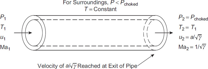
For long pipes or for large pressure differences across the pipe, the velocity of the gas can approach the sonic velocity. This case is shown in Figure 4-12.

Adiabatic choked flow of gas through a pipe is shown in a figure. — **Figure 4-12** Adiabatic choked flow of gas through a pipe. The sonic velocity is reached at the end of the pipe.

A figure shows the adiabatic choked flow of gas through a pipe. Various parameters related to the gas entering the pipe are, P1, T1, u1, and M a1. For surroundings, P is less than P subscript choked and Q equals 0. Sonic velocity is reached at the exit of the pipe. Various parameters related to the gas exiting the pipe are, P2 equals P subscript choked, T2, u2 equals sonic velocity, and M a2 equals 1.

When the sonic velocity is reached, the gas flow is called choked. The gas reaches the sonic velocity at the end of the pipe. If the upstream pressure is increased or if the downstream pressure is decreased, the gas velocity at the end of the pipe remains constant at the sonic velocity. If the downstream pressure is decreased below the choked pressure P_choked, the flow through the pipe remains choked and constant, independent of the downstream pressure. The pressure at the end of the pipe will remain at P_choked even if this pressure is greater than the ambient pressure. The gas exiting the pipe makes an abrupt change from P_choked to the ambient pressure. For choked flow, Equations 4-56 through 4-60 are simplified by setting Ma₂=1.0. The results are

$\begin{matrix} \begin{matrix} \frac{T_{c h o k e d}}{T_{1}} = \frac{2 Y_{1}}{γ + 1} \end{matrix} & (4-63) \end{matrix}$

$\begin{matrix} \begin{matrix} \frac{P_{c h o k e d}}{P_{1}} = {Ma}_{1} \sqrt{\frac{2 Y_{1}}{γ + 1}} \end{matrix} & (4-64) \end{matrix}$

$\begin{matrix} \begin{matrix} \frac{P_{c h o c k e d}}{ρ_{1}} = M a_{1} \sqrt{\frac{γ + 1}{2 Y_{1}}} \end{matrix} & (4-65) \end{matrix}$

$\begin{matrix} \begin{matrix} G_{choked} = ρ \bar{u} = {Ma}_{1} P_{1} \sqrt{\frac{γ g_{c} M}{R_{g} T_{1}}} = P_{choked} \sqrt{\frac{γ g_{c} M}{R_{g} T_{choked}}} \end{matrix} & (4-66) \end{matrix}$

$\begin{matrix} \begin{matrix} \frac{γ + 1}{2} \ln [\frac{2 Y_{1}}{(γ + {1)Ma}_{1}^{2}}] - (\frac{1}{{Ma}_{1}^{2}} - 1) + γ (\frac{4 f L}{d}) = 0 \end{matrix} & (4-67) \end{matrix}$

Choked flow occurs if the downstream pressure is less than P_choked. This is checked using Equation 4-64.

For most problems involving choked adiabatic flows, the pipe length (L), inside diameter (d), and upstream pressure (P₁) and temperature (T₁) are known. To compute the mass flux G, the procedure is as follows:

Determine the Fanning friction factor f using Equation 4-34. This assumes fully developed turbulent flow at high Reynolds numbers. This assumption can be checked later but is usually valid.
Determine Ma₁ from Equation 4-67.
Determine the mass flux G_choked from Equation 4-66.
Determine P_choked from Equation 4-64 to confirm operation at choked conditions.

Equations 4-63 through 4-67 for adiabatic pipe flow can be modified to use the 2-K method discussed previously by substituting $\sum K_{f}$ for 4fL/d.

The procedure can be simplified by defining a gas expansion factor Y_g. For ideal gas flow, the mass flow for both sonic and non-sonic conditions is represented by the Darcy formula:¹¹

¹¹Crane Co. Flow of Fluids through Valves, Fittings, and Pipes, Technical Paper 410 (New York, NY: Crane Co., 2009). www.flowoffluids.com.

$\begin{matrix} G = \frac{\dot{m}}{A} = Y_{g} \sqrt{\frac{2 g_{c} ρ_{1} (P_{1} - P_{2})}{Σ K_{f}}} & (4-68) \end{matrix}$

where

G is the mass flux (mass/area-time),

$\dot{m}$ is the mass flow rate of gas (mass/time),

A is the area of the discharge (length²),

Y_g is a gas expansion factor (unitless),

g_c is the gravitational constant (force/mass-acceleration),

ρ₁ is the upstream gas density (mass/volume),

P₁ is the upstream gas pressure (force/area),

P₂ is the downstream gas pressure (force/area), and

∑K_f are the excess head loss terms, including pipe entrances and exits, pipe lengths, and fittings (unitless).

The excess head loss terms ∑K_f are found using the 2-K method presented in Section 4-4. For most accidental discharges of gases, the flow is fully developed turbulent flow. Thus, for pipes, the friction factor is independent of the Reynolds number, and for fittings, K_f = K_∞ and the solution is direct.

The gas expansion factor Y_g in Equation 4-68 depends only on the heat capacity ratio of the gas γ and the frictional elements in the flow path ∑ K_f. An equation for the gas expansion factor for choked flow is obtained by equating Equation 4-68 to Equation 4-59 and solving for Y_g. The result is

$\begin{matrix} Y_{g} = {Ma}_{1} \sqrt{\frac{γ \sum K_{f}}{2} (\frac{P_{1}}{P_{1} - P_{2}})} & (4-69) \end{matrix}$

where Ma₁ is the upstream Mach number.

The procedure to determine the gas expansion factor is as follows. First, the upstream Mach number Ma₁ is determined using Equation 4-67. ∑K_f must be substituted for 4fL/d to include the effects of pipes and fittings. The solution is obtained by trial and error by guessing values of the upstream Mach number and determining whether the guessed value meets the equation objectives. This can be easily done using a spreadsheet.

The next step in the procedure is to determine the sonic pressure ratio, using Equation 4-64. If the actual ratio is greater than the ratio from Equation 4-64, then the flow is sonic or choked; the pressure drop predicted by Equation 4-64 is then used to continue the calculation. If the actual ratio is less than the ratio from Equation 4-64, then the flow is not sonic and the actual pressure drop ratio is used. Finally, the expansion factor Y_g is calculated from Equation 4-69.

The calculation to determine the expansion factor can be completed once γ and the frictional loss terms ∑K_f are specified. This computation can be done once and for all with the results shown in Figures 4-13 and 4-14. As shown in Figure 4-13, the pressure ratio (P − P₂)/P₁ is a weak function of the heat capacity ratio γ. The expansion factor Y_g has little dependence on γ, with the value of Y_g varying by less than 1% from the value at γ = 1.4 over the range from γ = 1.2 to γ = 1.67. Figure 4-14 shows the expansion factor for γ = 1.4.

A graph plots the pressure drop against velocity head loss. — **Figure 4-13** Pressure drop ratio as a function of the excess velocity head pipe losses for adiabatic flow. All values above the curve are sonic, while those below are not sonic. (Source: Adapted from J. M. Keith and D. A. Crowl. “Estimating Sonic Gas Flow Rates in Pipelines.” *Journal of Loss Prevention in the Process Industries* 18 (2005): 55–62.)

A graph of Pressure drop ratio against velocity head loss is shown. The horizontal axis represents velocity head loss, K subscript f, and ranges from 0.01 to 1000. The vertical axis represents pressure drop ratio, (p1 minus P2) times P1, and ranges from 0 to 1, in increments of 0.2. Three increasing curves representing the gamma values, 1.2, 1.4, and 1.67, respectively are drawn in the graph. Note: All the mentioned values are approximate.

A graph plots the expansion factor against velocity head loss. — **Figure 4-14** Gas expansion factor as a function of the excess velocity head pipe losses for adiabatic flow. The results are a weak function of heat capacity, but the difference is less than can be shown on this figure. (Source: Adapted from J. M. Keith and D. A. Crowl. “Estimating Sonic Gas Flow Rates in Pipelines.” *Journal of Loss Prevention in the Process Industries* 18 (2005): 55–62.)

A graph of Expansion factor, Y subscript g, against velocity head loss, K subscript f, is shown. The horizontal axis represents velocity head loss, K subscript f, and ranges from 0.01 to 1000. The vertical axis represents expansion factor, Y subscript g, and ranges from 0 to 0.8, in increments of 0.1. An increasing curve is drawn which passes through the following points, (0.01, 0.25), (10, 0.7), and (1000, 0.69). Note: All the mentioned values are approximate.

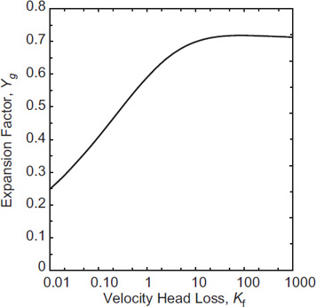
The functional results of Figures 4-13 and 4-14 can be fitted using an equation of the form ln Y_g = A(ln K_f)³ + B(ln K_f)² + C(ln K_f) + D, where A, B, C, and D are constants. The results are shown in Table 4-4 and are valid for the K_f ranges indicated, within 1%.

Table 4-4 Correlations for the Expansion Factor Y_g and the Sonic Pressure Drop Ratio (P₁ − P₂)/P₁ as a Function of the Pipe Loss ΣK_f for Adiabatic Flow Conditions^a

$\begin{matrix} {Expansion Factor: ln Y}_{g} = A (ln K_{f})^{3} + B (ln K_{f})^{2} + C (ln K_{f}) + D \\ Pressure Drop Ratio: [(P_{1} - P_{2} / P_{1})^{- 1} = A + B ln K_{f} + C / K_{f}^{0.5} \end{matrix}$

Function value	Range of validity, ∑K_f	A	B	C	D
Expansion factor, Y_g	0.2−1000	0.00129	−0.0216	0.116	−0.528
Sonic pressure drop ratio, γ = 1.2	0.01−1000	0.943	0.00762	1.12	–
Sonic pressure drop ratio, γ = 1.4	0.2−1000	0.965	0.00461	0.944	–
Sonic pressure drop ratio, γ = 1.67	0.01−1000	0.988	0.00113	0.768	–

^aJ. Keith and D. A. Crowl. “Estimating Sonic Gas Flow Rates in Pipelines,” Journal of Loss Prevention in the Process Industries 18 (2005): 55–62.

The procedure to determine the adiabatic mass flow rate through a pipe or hole is as follows:

Given M, γ based on the type of gas; pipe length, diameter, and type; pipe entrances and exits; total number and type of fittings; total pressure drop; and upstream gas density.
Assume fully developed turbulent flow to determine the friction factor for the pipe and the excess head loss terms for the fittings and pipe entrances and exits. The Reynolds number can be calculated at the completion of the calculation to check this assumption. Sum the individual excess head loss terms to get ∑K_f.
Calculate (P₁ − P₂)/P₁ from the specified pressure drop. Check this value against Figure 4-13 to determine whether the flow is sonic. All areas above the curves in Figure 4-13 represent sonic flow. Determine the sonic choking pressure P₂ by using Figure 4-13 directly, interpolating a value from the table, or using the equations provided in Table 4-4.
Determine the expansion factor from Figure 4-14. Either read the value off of the figure, interpolate it from the table, or use the equation provided in Table 4-4
Calculate the mass flow rate using Equation 4-68. Use the sonic choking pressure determined in step 3 in this expression

This method is applicable to gas discharges through piping systems and holes.

Isothermal Flows

Isothermal flow of gas in a pipe with friction is shown in Figure 4-15. For this case, the gas velocity is assumed to be well below the sonic velocity of the gas. A pressure gradient across the pipe provides the driving force for the gas transport. As the gas expands through the pressure gradient, the velocity must increase to maintain the same mass flow rate. The pressure at the end of the pipe is equal to the pressure of the surroundings. The temperature is constant across the entire pipe length.

Isothermal nonchoked flow of gas through a pipe is shown in a diagram. — **Figure 4-15** Isothermal nonchoked flow of gas through a pipe.

A diagram illustrates the isothermal nonchoked flow of gas through a pipe. Variable parameters representing the gas entering the pipe are, P1, u overbar 1, and M a1. The temperature T equals constant, for the entire pipe. The length of the pipe is, L. Variable parameters related to the air leaving the pipe are, P2 less than P1, P2 less than P subscript choked, u overbar 2 less than sonic velocity, u overbar 2, less than u overbar 1, M a2 less than Ma1, and M a2 less than 1. For surroundings, P equals P2 less than P subscript choked.

Isothermal flow is represented by the mechanical energy balance in the form shown in Equation 4-54. The following assumptions are valid for this case:

$\frac{g}{g_{c}} d z = 0$

is valid for gases, and, by combining Equations 4-29 and 4-30 and differentiating,

$d F = \frac{2 f {\bar{u}}^{2}}{g_{c} d} d L$

assuming constant f, and

$δ W_{S} = 0$

because no mechanical linkages are present. A total energy balance is not required because the temperature is constant.

By applying the assumptions to Equation 4-54 and manipulating them considerably, we obtain¹²

¹²Octave Levenspiel. Engineering Flow and Heat Exchange, 2nd ed. (New York, NY: Springer, 1998), p. 46.

$\begin{matrix} \begin{matrix} T_{2} = T_{1} \end{matrix} & (4-70) \end{matrix}$

$\begin{matrix} \begin{matrix} \frac{P_{2}}{P_{1}} = \frac{{Ma}_{1}}{{Ma}_{2}} \end{matrix} & (4-71) \end{matrix}$

$\begin{matrix} \begin{matrix} \frac{ρ_{2}}{ρ_{1}} = \frac{{Ma}_{1}}{{Ma}_{2}} \end{matrix} & (4-72) \end{matrix}$

$\begin{matrix} \begin{matrix} \begin{matrix} G = ρ \bar{u} = M a_{1} P_{1} \sqrt{\frac{γ g_{c} M}{R_{g} T}} \end{matrix} \end{matrix} & (4-73) \end{matrix}$

where G is the mass flux with units of mass/(area-time), and

$\begin{matrix} \begin{matrix} \begin{array}{l} 2 \ln \frac{{Ma}_{2}}{{Ma}_{1}} - \frac{1}{γ} (\frac{1}{{Ma}_{1}^{2}} - \frac{1}{{Ma}_{2}^{2}}) + \frac{4 f L}{d} = 0 \\ Kinetic Compressibility Friction \end{array} \end{matrix} & (4-74) \end{matrix}$

The various energy terms in Equation 4-74 have been identified.

A more convenient form of Equation 4-74 is expressed in terms of pressure instead of Mach numbers. This form is derived using Equations 4-70 through 4-72. The result is

$\begin{matrix} \begin{matrix} 2 \ln \frac{P_{1}}{P_{2}} - \frac{g_{c} M}{G^{2} R_{g} T} (P_{1}^{2} - P_{2}^{2}) + \frac{4 f L}{d} = 0 \end{matrix} & (4-75) \end{matrix}$

A typical problem is to determine the mass flux G given the pipe length (L), inside diameter (d), and upstream and downstream pressures (P₁ and P₂). The procedure is as follows:

Determine the Fanning friction factor f using Equation 4-34. This assumes fully developed turbulent flow at high Reynolds numbers. This assumption can be checked later but is usually valid.
Compute the mass flux G from Equation 4-75.

Levenspiel¹³ showed that the maximum velocity possible during the isothermal flow of gas in a pipe is not the sonic velocity, as in the adiabatic case. In terms of the Mach number, the maximum velocity is

¹³Octave Levenspiel. Engineering Flow and Heat Exchange, 2nd ed. (New York, NY: Springer, 1998), p. 46.

$\begin{matrix} {Ma}_{choked} = \frac{1}{\sqrt{γ}} & (4-76) \end{matrix}$

This result is shown by starting with the mechanical energy balance and rearranging it into the following form:

$\begin{matrix} - \frac{d P}{d L} = \frac{2 f G^{2}}{g_{c} ρ d} [\frac{1}{1 - ({\bar{u}}^{2} ρ / g_{c} P)}] = \frac{2 f G^{2}}{g_{c} ρ d} (\frac{1}{1 - γ {Ma}^{2}}) & (4-77) \end{matrix}$

The quantity – (dP/dL)→ ∞ when $Ma \to 1/ \sqrt{γ}$ . Thus, for choked flow in an isothermal pipe, as shown in Figure 4-16, the following equations apply:

Isothermal choked flow of gas through a pipe is represented in a figure. — **Figure 4-16** Isothermal choked flow of gas through a pipe. The maximum velocity is reached at the end of the pipe.

A figure shows the isothermal choked flow of gas through a pipe. Various parameters related to the gas entering the pipe are, P1, T1, u1, and Ma1. Various parameters related to the gas leaving the pipe are, P2 equals P subscript choked, T2 equals T1, u2 equals 'a' slash Square root of gamma, and Ma2 equals 1 slash square root of gamma. Velocity of 'a' slash square root of gamma, is reached at the exit of the pipe. For surroundings, P is less than P subscript choked, and T is constant.

$\begin{matrix} \begin{matrix} T_{choked} = T_{1} \end{matrix} & (4-78) \end{matrix}$

$\begin{matrix} \begin{matrix} \frac{P_{choked}}{P_{1}} = {Ma}_{1} \sqrt{γ} \end{matrix} & (4-79) \end{matrix}$

$\begin{matrix} \frac{ρ_{choked}}{ρ_{1}} = {Ma}_{1} \sqrt{γ} & (4-80) \end{matrix}$

$\begin{matrix} \begin{matrix} \frac{{\bar{u}}_{choked}}{{\bar{u}}_{1}} = \frac{1}{{Ma}_{1} \sqrt{γ}} \end{matrix} & (4-81) \end{matrix}$

$\begin{matrix} \begin{matrix} G_{choked} = ρ \bar{u} = ρ_{1} {\bar{u}}_{1} = {Ma}_{1} P_{1} \sqrt{\frac{γ g_{c} M}{R_{g} T}} = P_{choked} \sqrt{\frac{g_{c} M}{R_{g} T}} \end{matrix} & (4-82) \end{matrix}$

where G_choked is the mass flux with units of mass/(area-time), and

$\begin{matrix} \begin{matrix} ln (\frac{1}{γ M a_{1}^{2}}) - (\frac{1}{γ M a_{1}^{2}} - 1) + \frac{4 f L}{d} = 0 \end{matrix} & (4-83) \end{matrix}$

For most typical problems, the pipe length (L), inside diameter (d), upstream pressure (P₁), and temperature (T) are known. The mass flux G is determined using the following procedure:

Determine the Fanning friction factor using Equation 4-34. This assumes fully developed turbulent flow at high Reynolds numbers. This assumption can be checked later but is usually valid.
Determine Ma₁ from Equation 4-83.
Determine the mass flux G from Equation 4-82.

The direct method using Equations 4-68 and 4-69 can also be applied to isothermal flows. Table 4-5 provides the equations for the expansion factor and the pressure drop ratio. Figures 4-17 and 4-18 are plots of these functions. The procedure is identical to the procedure for adiabatic flows.

An increasing curve is plotted in a graph of pressure drop ratio versus velocity head loss. — **Figure 4-17** Pressure drop ratio as a function of the excess velocity head pipe losses for isothermal flow. The results are independent of the heat capacity ratio. All values above the curve are sonic, while those below are not sonic. (Source: Adapted from J. M. Keith and D. A. Crowl. “Estimating Sonic Gas Flow Rates in Pipelines.” *Journal of Loss Prevention in the Process Industries* 18 (2005): 55–62.)

A graph of Pressure drop ratio against velocity head loss is shown. The horizontal axis represents velocity head loss, K subscript f, and ranges from 0.01 to 1000. The vertical axis represents pressure drop ratio, (P1 P2) times P1, and ranges from 0 to 1, in increments of 0.2. An increasing curve is plotted which passes through the following points, (0.01, 0.08), (10, 0.75), and (1000, 0.97). Note: All the mentioned values are approximate.

A graph plots the expansion factor versus velocity head loss. — **Figure 4-18** Gas expansion factor as a function of the excess velocity head pipe losses for isothermal flow. The results are independent of the heat capacity ratio. (Source: Adapted from J. M. Keith and D. A. Crowl. “Estimating Sonic Gas Flow Rates in Pipelines.” *Journal of Loss Prevention in the Process Industries* 18 (2005): 55–62.)

A graph of Expansion factor against velocity head loss is shown. The horizontal axis represents the velocity head loss, K subscript f, and ranges from 0.01 to 1000. The vertical axis represents the expansion factor, Y subscript g, and ranges from 0 to 0.8, in increments of 0.1. An increasing curve is plotted, which passes through the following points, (0.01, 0.26), (10, 0.73), and (1000, 7.2). Note: All the mentioned values are approximate.

Table 4-5 Correlations for the Expansion Factor Y_g and the Sonic Pressure Drop Ratio (P₁ − P₂)/P₁ as a Function of the Pipe Loss ΣK_f for Isothermal Flow Conditions^a

$\begin{matrix} Expansion Factor : & \ln Y_{g} = A {(\ln K_{f})}^{3} + B {(\ln k_{f})}^{2} + C (\ln K_{f}) + D \\ Pressure Drop Ratio : & {\begin{matrix} [(P_{1} - P_{2}) / P_{1}] \end{matrix}}^{- 1} = A + B \ln k_{f} + C / K_{f}^{0.5} \end{matrix}$

Function value	Range of validity, ∑K_f	A	B	C	D
Expansion factor Y_g	0.2−1000	0.00130	−0.0216	0.111	−0.502
Sonic pressure drop ratio, all γ	0.01−1000	0.911	0.0118	1.38	−

^aJ. Keith and D. A. Crowl. “Estimating Sonic Gas Flow Rates in Pipelines,” Journal of Loss Prevention in the Process Industries 18 (2005): 55–62.

Keith and Crowl¹⁴ found that for both the adiabatic and isothermal cases, the expansion factor Y_g exhibits a maximum value. For isothermal flows, this maximum is the same for all values of the heat capacity ratio γ and occurs at a velocity head loss of 56.3 with a maximum expansion factor of 0.7248. For adiabatic flows, the maximum value of the expansion factor is a function of the heat capacity ratio γ. For γ = 1.4, the expansion factor has a maximum value of 0.7182 at a velocity head loss of 90.0.

¹⁴J. Keith and D. A. Crowl. “Estimating Sonic Gas Flow Rates in Pipelines,” Journal of Loss Prevention in the Process Industries 18 (2005): 55–62.

For both the adiabatic and isothermal flow cases, the expansion factor approaches an asymptote as the velocity head loss becomes large. This asymptote, $1/ \sqrt{2} = 0.7071$ , is the same for both the adiabatic and isothermal flow cases. Comparison of detailed calculations with the asymptotic solution show that for velocity head loss values of 100 and 500, the differences between the detailed and asymptotic solutions are 2.2% and 0.2%, respectively.

The asymptotic solution can be inserted into Equation 4-68 to result in the following simplified equation for the mass flow:

$\begin{matrix} G = \frac{\dot{m}}{A} = \sqrt{\frac{g_{c} ρ_{1} P_{1}}{\sum K_{f}}} & (4-84) \end{matrix}$

For gas releases through pipes, the issue of whether the release occurs adiabatically or isothermally is important. For both cases, the velocity of the gas increases because of the expansion of the gas as the pressure decreases. For adiabatic flows, the temperature of the gas may increase or decrease, depending on the relative magnitude of the frictional and kinetic energy terms. For choked flows, the adiabatic choking pressure is less than the isothermal choking pressure. For real pipe flows from a source at a fixed pressure and temperature, the actual flow rate is less than the adiabatic prediction and greater than the isothermal prediction.

Example 4-5 shows that for pipe flow problems, the difference between the adiabatic and isothermal results is generally small. Levenspiel¹⁵ showed that the adiabatic model always predicts a flow larger than the actual flow, provided that the source pressure and temperature are the same. Crane¹⁶ reported that adiabatic conditions are valid for short pipes of constant cross-sectional are discharging into a pipe or area of larger cross-section. Crane supported this conclusion with experimental data on pipes having lengths of 130 and 220 pipe diameters discharging air to the atmosphere. Finally, under choked sonic flow conditions, isothermal conditions are difficult to achieve practically because of the rapid speed of the gas flow. As a result, the adiabatic flow model is the model of choice for compressible gas discharges through pipes.

¹⁵Octave Levenspiel. Engineering Flow and Heat Exchange, 2nd ed. (New York, NY: Springer, 1998), p. 45.

¹⁶Crane Co. Flow of Fluids through Valves, Fittings, and Pipes, Technical Paper 410 (New York, NY: Crane Co., 2009). www.flowoffluids.com.

Example 4-5

The vapor space above liquid ethylene oxide (EO) in storage tanks must be purged of oxygen and then padded with 81 psig nitrogen to prevent explosion. The nitrogen in a particular facility is supplied from a 200 psig source. It is regulated to 81 psig and supplied to the storage vessel through 33 ft of new commercial steel pipe with an internal diameter of 1.049 in. The temperature is 80°F.

In the event that the nitrogen regulator fails, the vessel will be exposed to the full 200 psig pressure from the nitrogen source. This will exceed the pressure rating of the storage vessel. To prevent rupture of the storage vessel, it must be equipped with a relief device to vent this nitrogen. Determine the required minimum mass flow rate of nitrogen through the relief device to prevent the pressure from rising within the tank in the event of a regulator failure.

Determine the mass flow rate assuming (a) an orifice with a throat diameter equal to the pipe diameter, (b) an adiabatic pipe, and (c) an isothermal pipe. Decide which result most closely corresponds to the real situation. Which mass flow rate should be used?

Solution

The maximum flow rate through the orifice occurs under choked conditions. The area of the pipe is

$\begin{array}{l} A = \frac{π d^{2}}{4} = \frac{(3.14) {(1.049 in)}^{2} (1 {ft}^{2} / {144 in}^{2})}{4} \\ = 6.00 \times 10^{- 3} {ft}^{2} \end{array}$

The absolute pressure of the nitrogen source is

$P_{1} = 200 + 14.7 = 214.7 psia = 3.09 \times 10^{4} {lb}_{f} {/ft}^{2}$

The choked pressure from Equation 4-49 is, for a diatomic gas,

$P_{choked} = (0.528) (214.7 psia) = 113.4 psia=1.63 \times 10^{4} 1 b_{f} / {ft}^{2}$

Choked flow can be expected because the system is venting to atmospheric conditions. Equation 4-50 provides the maximum mass flow rate. For nitrogen, γ = 1.41 (Table 4-3) and

${(\frac{2}{γ +1})}^{(γ +1)/(γ - 1)} = {(\frac{2}{2.41})}^{2.41/0.41} = 0.335$

The molecular weight of nitrogen is 28 lb_m/lb-mol. Without any additional information, assume a unit discharge coefficient C₀=1.0. Thus

$\begin{matrix} \begin{array}{l} \end{array} Q_{m} & = (1.0)(6.00 \times 10^{- 3} {ft}^{2}) \\ \times (3.09 \times 10^{4} {1b}_{f} {/ft}^{2}) \times \sqrt{\frac{{(1.41)(32.17 ft 1b}_{m} {/1b}_{f} s^{2} {)(28 1b}_{m} /1b-mole)}{{(1545 ft 1b}_{f} {/1b-mole}^{o} {R)(540}^{o} R)} (0.335)} \\ = ({185 1b}_{f}) \sqrt{5.08 \times 10^{- 4} {lb}_{m}^{2} {/1b}_{f}^{2} s^{2}} \\ Q_{m} & = {4.17 1b}_{m} /s \end{matrix}$
Assume adiabatic choked flow conditions. For commercial steel pipe, from Table 4-1, ε = 0.046 mm. The diameter of the pipe in millimeters is (1.049 in) (25.4 mm/in) = 26.6 mm. Thus

$\frac{ε}{d} = \frac{0.046 m m}{26.6 m m} = 0.00173$

From Equation 4-34,

$\begin{matrix} \frac{1}{\sqrt{f}} & = 4 \log (3.7 \frac{d}{ε}) \\ = 4 \log (3.7/0.00173) = 13.32 \\ \sqrt{f} & = 0.0751 \\ f & = 0.00564 \end{matrix}$

As stated previously for nitrogen, γ = 1.41.

The upstream Mach number is determined from Equation 4-67:

$\frac{γ + 1}{2} \ln [\frac{2 Y_{1}}{(γ + {1)Ma}_{1}^{2}}] - (\frac{1}{{Ma}_{1}^{2}} - 1) + γ (\frac{4 f L}{d}) = 0$

with Y₁ given by Equation 4-56. Substituting the numbers provided gives

$\begin{array}{l} \frac{1.4 1 + 1}{2} \ln [\frac{2 + (1.41 - {1) Ma}^{2}}{(1.41 + {1) Ma}^{2}}] - (\frac{1}{{Ma}^{2}} - 1) +1.41 [\frac{(4)(0.00564)(33 ft)}{(1.049 in)(1 ft/12 in)}] = 0 \\ 1.2 \ln (\frac{2 + {0.41 Ma}^{2}}{{2.41 Ma}^{2}}) - (\frac{1}{{Ma}^{2}} - 1) + 12.01 = 0 \end{array}$

This equation is solved by trial and error or a solver program or spreadsheet for the value of Ma. The results are tabulated as follows:

Guessed Ma

Value of left-hand side of equation

0.20

−8.34

0.25

0.128

0.249

0.0093

This last guessed Mach number gives a result close to zero. Then, from Equation 4-56,

$Y_{1} = 1 + \frac{γ + 1}{2} {Ma}^{2} = 1 + \frac{1.41-1}{2} {(0.249)}^{2} = 1.013$

and from Equations 4-63 and 4-64,

$\begin{array}{l} \frac{T_{choked}}{T_{1}} = \frac{2 Y_{1}}{γ + 1} = \frac{2 (1.013)}{1.41 + 1} = 0.841 \\ T_{choked} = (0.841) {(80 + 460)}^{o} R = 454^{o} R \\ \frac{P_{choked}}{P_{1}} = Ma \sqrt{\frac{2 Y_{1}}{γ + 1}} = (0.249) \sqrt{0.841} = 0.228 \\ P_{choked} = (0.228) (214.7 psia) = 48.9 psia = 7.05 \times 10^{3} {lb}_{f} / {ft}^{2} \end{array}$

The pipe outlet pressure must be less than 48.9 psia to ensure choked flow. The mass flux is computed using Equation 4-66:

$\begin{matrix} G_{choked} & = P_{choked} \sqrt{\frac{γ g_{c} M}{R_{g} T_{choked}}} \\ = (7.05 \times 10^{3} {1b}_{f} {/ft}^{2}) \sqrt{\frac{{(1.41)(32.17 ft 1b}_{m} {/1b}_{f} s^{2} {)(28 1b}_{m} /1b-mole)}{{(1545 ft 1b}_{f} {/1b-mole}^{o} {R)(454}^{o} R)}} \\ = 7.05 \times 10^{3} {1b}_{f} {/ft}^{2} \sqrt{1.81 \times 10^{- 3} {lb}_{m}^{2} / {lb}_{f}^{2} s^{2}} = {300 1b}_{m} {/ft}^{2} s \\ Q_{m} & = G A = {(300 lb}_{m} {/ft}^{2} s)(6.00 \times 10^{- 3} {ft}^{2}) \\ = {1.80 1b}_{m} /s \end{matrix}$

The simplified procedure with a direct solution can also be used. The excess head loss resulting from the pipe length is given by Equation 4-30. The friction factor f has already been determined:

$k_{f} = \frac{4 f L}{d} = \frac{(4) (0.00564) (33 ft) (12 in / ft)}{1.049 in} = 8.52$

For this solution, only the pipe friction will be considered and the exit effects will be ignored. The first consideration is whether the flow is sonic. The sonic pressure ratio is given in Figure 4-13 (or the equations in Table 4-4). For γ = 1.41, K_f = 8.52 and P₂ = 214.7 psia:

$\frac{P_{1} - P_{2}}{P_{1}} = 0.770 \to P_{2} = 49.4 psia$

It follows that the flow is sonic because the downstream pressure is less than 49.4 psia. From Figure 4-14 (or Table 4-4), the gas expansion factor Y_g = 0.69. The gas density under the upstream conditions is

$ρ_{1} = \frac{P_{1} M}{R_{g} T} = \frac{(214.7 psia) (28 {lb}_{m} /lb-mole)}{(10.731 {psia ft}^{3} / {lb-mole}^{o} R) (540^{o} R)} = 1.037 {lb}_{m} {/ft}^{3}$

By substituting this value into Equation 4-68 and using the choking pressure determined for P₂, we obtain

$\begin{matrix} \dot{m} & = Y_{g} A \sqrt{\frac{2 g_{c} ρ_{1} (P_{1} - P_{2})}{\sum K_{f}}} \\ = (0.69)(6.00 \times 10^{- 3} {ft}^{2}) \sqrt{\frac{2 (32.17 \frac{{ft 1b}_{m}}{{1b}_{f} s^{2}}) (1.037 \frac{{1b}_{m}}{{ft}^{3}}) (214.7 - 49.4) (\frac{{1b}_{f}}{{in}^{2}}) (144 \frac{{in}^{2}}{{ft}^{2}})}{8.56}} \\ = {1.78 1b}_{m} /s \end{matrix}$

This result is very close to the previous result, but requires a lot less effort to obtain.
For the isothermal case, the upstream Mach number is given by Equation 4-83. Substituting the numbers provided, we obtain

Guessed Ma	Value of left-hand side of equation
0.20	−8.34
0.25	0.128
0.249	0.0093

$\ln (\frac{1}{1.41 {Ma}^{2}}) - (\frac{1}{1.41 {Ma}^{2}} - 1) + 8.52 = 0$

The solution is found by trial and error:

Guessed Ma	Value of left-hand side of equation
0.25	0.601
0.24	−0.282
0.245	0.174
0.244	0.085
0.243	−0.005← Final result

The choked pressure is, from Equation 4-79,

$P_{choked} = P_{1} {Ma}_{1} \sqrt{γ} = {(214.7 1b}_{f} {/in}^{2})(0.243) \sqrt{1.41} = 62.0 psia = 8.93 \times 10^{3} {1b}_{f} {/ft}^{2} .$

The mass flow rate is computed using Equation 4-82:

$\begin{matrix} G_{choked} & = P_{choked} \sqrt{\frac{g_{c} M}{R_{g} T}} = 8.93 \times 10^{3} 1 b_{f} / {ft}^{2} \times \sqrt{\frac{(32.17 ft 1 b_{m} / 1 b_{f} s^{2}) (28 1 b_{m} / 1 b-mole)}{(1545 ft 1 b_{f} / 1 b- {mole}^{o} R) (540^{o} R)}} \\ = 8.93 \times 10^{3} 1 b_{f} / f t^{2} \sqrt{1.08 \times 10^{- 3} 1 b_{m}^{2} / 1 b_{f}^{2}} = 293 1 b_{m} / f t^{2} s \\ Q_{m} & = G_{choked} A = (293 1 b_{m} / f t^{2} s) (6.00 \times 10^{- 3} f t^{2}) \\ = 1.76 1 b_{m} / s \end{matrix}$

Using the simplified, direct solution, from Table 4-5 or Figure 4-15,

$\frac{P_{1} - P_{2}}{P_{1}} = 0.70 \Rightarrow P_{2} = 64.4 psia$

It follows that the flow is sonic. From Table 4-5 or Figure 4-16, Y_g = 0.70. Substituting into Equation 4-68, and remembering to use the choking pressure given earlier, gives $\dot{m} = 1.74 {1b}_{m} /s$ . This is also very close to the more detailed method.

The results are summarized in the following table:

Case	P_choked (psia)	Q_m (lb_m/s)
a. Orifice	113.4	4.17
b. Adiabatic pipe Simplified	48.9 113.4	1.80 1.78
c. Isothermal pipe Simplified	62.0 64.4	1.76 1.74

Case

P_choked

(psia)

Q_m

(lb_m/s)

a. Orifice

113.4

4.17

b. Adiabatic pipe
Simplified

48.9
113.4

1.80
1.78

c. Isothermal pipe
Simplified

62.0
64.4

1.76
1.74

A standard procedure for these types of problems is to represent the discharge through the pipe as an orifice. The results obtained earlier show that this approach results in a large mass flow rate for this case. The orifice method always produces a larger value than the adiabatic pipe method, ensuring a conservative safety design. The orifice calculation, however, is easier to apply, requiring only the pipe diameter and the upstream supply pressure and temperature. The configurational details of the piping are not required, as in the adiabatic and isothermal pipe methods.

Also note that the computed choked pressures differ for each case, with a substantial difference between the orifice and the adiabatic and isothermal cases. A choking design based on an orifice calculation might not be choked in reality because of high downstream pressures.

Both the adiabatic and isothermal pipe methods produce results that are reasonably close. For most real-world situations, the heat transfer characteristics cannot be easily determined. Thus, the adiabatic pipe method is the method of choice; it will always produce the larger number for a conservative safety design.

Finally, the simplified adiabatic and isothermal methods produce almost the same results as the more detailed approach.

4-7 Flashing Liquids

Liquids stored under pressure above their normal boiling point temperature present substantial problems because of flashing. If the tank, pipe, or other containment device develops a leak, the liquid will partially flash into vapor, sometimes explosively.

Flashing occurs so rapidly that the process is assumed to be adiabatic. The excess energy contained in the superheated liquid vaporizes the liquid and lowers the temperature to the new boiling point. If m is the mass of original liquid, C_p is the heat capacity of the liquid (energy/mass degrees), T_o is the initial temperature of the liquid before depressurization, and T_b is the depressurized boiling point of the liquid, then the excess energy contained in the superheated liquid is given by

$\begin{matrix} Q = m C_{p} (T_{o} - T_{b}) & (4-85) \end{matrix}$

This energy vaporizes the liquid. If ΔH_v is the heat of vaporization of the liquid, the mass of liquid vaporized m_v is given by

$\begin{matrix} m_{v} = \frac{Q}{Δ H_{v}} = \frac{m C_{p} (T_{o} - T_{b})}{Δ H_{v}} & (4-86) \end{matrix}$

The fraction of the liquid vaporized is

$\begin{matrix} f_{v} = \frac{m_{v}}{m} = \frac{C_{p} (T_{o} - T_{b})}{Δ H_{v}} & (4-87) \end{matrix}$

Equation 4-87 assumes constant physical properties over the temperature range T_o to T_b. A more general expression without this assumption is derived as follows. The change in liquid mass m resulting from a change in temperature T is given by

$\begin{matrix} d m = \frac{m C_{p}}{Δ H_{v}} d T & (4-88) \end{matrix}$

Equation 4-88 is integrated between the initial temperature T_o (with liquid mass m) and the final boiling point temperature T_b (with liquid mass m − m_v):

$\begin{matrix} \int_{m}^{m - m_{v}} \frac{d m}{m} = \int_{T_{o}}^{T_{b}} \frac{C_{P}}{Δ H_{v}} d T & (4-89) \end{matrix}$

$\begin{matrix} ln (\frac{m - m_{v}}{m}) = \frac{{\bar{C}}_{p} (T_{o} - T_{b})}{{\bar{Δ H}}_{v}} & (4-90) \end{matrix}$

where $\bar{C_{p}}$ and $\bar{Δ H_{v}}$ are the mean heat capacity and the mean latent heat of vaporization, respectively, over the temperature range T_o to T_b. Solving for the fraction of the liquid vaporized, f_v = m_v/m, we obtain

$\begin{matrix} f_{v} = 1 - exp [- \bar{C_{p}} (T_{o} - T_{b}) / \bar{Δ H_{v}}] & (4-91) \end{matrix}$

Example 4-6

One lb_m of saturated liquid water is contained in a vessel at 350°F. The vessel ruptures and the pressure is reduced to 1 atm. Compute the fraction of material vaporized using (a) the steam tables,
(b) Equation 4-87, and (c) Equation 4-91.

Solution

The initial state is saturated liquid water at T_o = 350°F. From the steam tables:

$\begin{matrix} P & = 134.6 psia \\ H & = 321.6 Btu/1 b_{m} \end{matrix}$

The final temperature is the boiling point at 1 atm, or 212°F. At this temperature and under saturated conditions, from the steam tables,

$\begin{matrix} H_{vapor} & = 1150.4 Btu/1 b_{m} \\ H_{liquid} & = 180.07 Btu/1 b_{m} \end{matrix}$

Because the process occurs adiabatically, H_final = H_initial and the fraction of vapor (or quality) is computed from

$\begin{matrix} H_{final} & = H_{liquid} + f_{v} (H_{vapor} - H_{liquid}) \\ 321.6 & = 180.07 + f_{v} (1150.4-180.07) \end{matrix} \begin{matrix} f_{v} & = 0.146 \end{matrix}$

That is, 14.6% of the mass of the original liquid is vaporized.
For liquid water at 212°F,

$\begin{matrix} C_{P} & = 1.01 Btu/1bm ° F \\ Δ H_{v} & = 970.3 {Btu/1b}_{m} \end{matrix}$

From Equation 4-87,

$f_{v} = \frac{C_{P} (T_{o} - T_{b})}{Δ H_{v}} = \frac{(1.01 BTU/1 b_{m} {}^{o}F) {(350-212)}^{o} F}{970.3 BTU/1 b_{m}}$

$\begin{matrix} f_{v} = 0.144 \end{matrix}$
The mean properties for liquid water between T_o and T_b are

$\begin{array}{l} \bar{C_{p}} = {1.04 BTU/1b}_{m}^{o} F \\ \bar{Δ H_{v}} = {920.7 BTU/1b}_{m} \end{array}$

Substituting into Equation 4-91 gives

$\begin{matrix} f_{v} & = 1 - \exp [- \bar{C_{P}} (T_{o} - T_{b}) / \bar{Δ H_{v}}] \\ = 1 - exp[- (1.04 {BTU/1b}_{m} ° F) (350-212) ° F/920.7 {BTU/1b}_{m}] \\ = 1-0.8557 \end{matrix}$

$\begin{matrix} f_{v} = 0.144 \end{matrix}$

The two methods using the equations produce results that are comparable to the actual value from the steam table. This agreement is not expected as one nears the critical temperature since the properties of the steam are changing rapidly.

For flashing liquids composed of many miscible substances, the flash calculation is complicated considerably, because the more volatile components flash preferentially. Procedures are available to solve this problem.¹⁷

¹⁷J. M. Smith and H. C. Van Ness. Introduction to Chemical Engineering Thermodynamics, 6th ed. (New York, NY: McGraw-Hill, 2000).

Flashing liquids escaping through holes and pipes require special consideration because two-phase flow conditions may be present. Several special cases may arise.¹⁸ If the fluid path length of the release is short (through a hole in a thin-walled container), nonequilibrium conditions exist, and the liquid does not have time to flash within the hole; instead, the fluid flashes external to the hole. The equations describing incompressible fluid flow through holes apply in this scenario (see Section 4-2).

¹⁸Hans K. Fauske. “Flashing Flows or: Some Practical Guidelines for Emergency Releases.” Plant/ Operations Progress (July 1985): 133.

If the fluid path length through the release is greater than 10 cm (through a pipe or thick-walled container), equilibrium flashing conditions are achieved and the flow is choked. A good approximation is to assume a choked pressure equal to the saturation vapor pressure of the flashing liquid. The result will be valid only for liquids stored at a pressure higher than the saturation vapor pressure. With this assumption the mass flow rate is given by

$\begin{matrix} Q_{m} = A C_{o} \sqrt{2 ρ_{f} g_{c} (P - P^{sat})} & (4-92) \end{matrix}$

where

A is the area of the release,

C_o is the discharge coefficient (unitless),

ρ_f is the density of the liquid (mass/volume),

P is the pressure within the tank, and

P^sat is the saturation vapor pressure of the flashing liquid at ambient temperature.

Example 4-7

Liquid ammonia is stored in a tank at 24°C and a pressure of 1.4 × 10⁶ Pa. A pipe of diameter 0.0945 m breaks off a short distance from the tank, allowing the flashing ammonia to escape. The saturation vapor pressure of liquid ammonia at this temperature is 0.968 × 10⁶ Pa, and its density is 603 kg/m³. Determine the mass flow rate through the leak. Equilibrium flashing conditions can be assumed.

Solution

Equation 4-92 applies for the case of equilibrium flashing conditions. Assume a discharge coefficient of 0.61. Substituting into Equation 4-92,

$\begin{matrix} Q_{m} & = A C_{o} \sqrt{2 ρ_{f} g_{c} (P - P^{sat})} \\ = \frac{(3.14) {(0.0945 m)}^{2}}{4} (0.61) \\ \times \sqrt{2 ({603 kg/m}^{3}) [1 ({kg m/s}^{2}) /N] (1.4 \times 10^{6} - 0.968 \times 10^{6}) ({N/m}^{2})} \\ Q_{m} & = 97.6 kg/s \end{matrix}$

For liquids stored at their saturation vapor pressure, P = P^sat, and escaping through a longer pipe, the liquid flashes in the pipe as the pressure in the pipe decreases. Equation 4-92 is no longer valid. An example of this would be liquid propane stored under its own vapor pressure escaping to atmospheric pressure through a pipe section. A much more detailed approach is required for this case.

Consider a fluid that is initially quiescent and is accelerated through the leak. Assume that kinetic energy is dominant and that potential energy effects are negligible. Then, from a mechanical energy balance (Equation 4-1), and realizing that the specific volume (with units of volume/mass) v = 1/ρ, we can write

$\begin{matrix} - \int_{1}^{2} v d P = \frac{{\bar{u}}_{2}^{2}}{2 g_{c}} & (4-93) \end{matrix}$

A mass velocity G with units of mass/(area-time) is defined by

$\begin{matrix} G = ρ \bar{u} = \frac{\bar{u}}{v} & (4-94) \end{matrix}$

Combining Equation 4-94 with Equation 4-93 and assuming that the mass velocity is constant results in

$\begin{matrix} - \int_{1}^{2} v d P = \frac{{\bar{u}}_{2}^{2}}{2 g_{c}} = \frac{G^{2} v_{2}^{2}}{2 g_{c}} & (4-95) \end{matrix}$

Solving for the mass velocity G and assuming that point 2 can be defined at any point along the flow path, we obtain

$\begin{matrix} G = \frac{\sqrt{- 2 g_{c} \int v d P}}{v} & (4-96) \end{matrix}$

Equation 4-96 contains a maximum, at which choked flow occurs. Under choked flow conditions, dG/dP = 0. Differentiating Equation 4-96 and setting the result equal to zero gives

$\begin{matrix} \frac{d G}{d P} = 0 = - \frac{(d v / d P)}{v^{2}} \sqrt{- 2 g_{c} \int v d P} - \frac{g_{c}}{\sqrt{- 2 g_{c} \int v d P}} & (4-97) \end{matrix}$

$\begin{matrix} 0 = - \frac{G (d v / d P)}{v} - \frac{g_{c}}{v G} & (4-98) \end{matrix}$

Solving Equation 4-98 for G, we obtain

$\begin{matrix} G = \frac{Q_{m}}{A} = \sqrt{- \frac{g_{c}}{(d v / d P)}} & (4-99) \end{matrix}$

The two-phase specific volume is given by

$\begin{matrix} v = v_{fg} f_{v} + v_{f} & (4-100) \end{matrix}$

where

v_fg is the difference in specific volume between vapor and liquid,

v_f is the liquid specific volume, and

f_v is the mass fraction of vapor.

Differentiating Equation 4-100 with respect to pressure gives

$\begin{matrix} \frac{d v}{d P} = v_{fg} \frac{d f_{v}}{d P} & (4-101) \end{matrix}$

But, from Equation 4-87,

$\begin{matrix} d f_{v} = - \frac{C_{P}}{Δ H_{v}} d T & (4-102) \end{matrix}$

and from the Clausius–Clapeyron equation, at saturation

$\begin{matrix} \frac{d P}{d T} = \frac{Δ H_{v}}{T v_{fg}} & (4-103) \end{matrix}$

Substituting Equations 4-103 and 4-102 into Equation 4-101 yields

$\begin{matrix} \frac{d v}{d P} = - \frac{v_{fg}^{2}}{Δ H_{v}^{2}} T C_{P} & (4-104) \end{matrix}$

The mass flow rate is determined by combining Equation 4-104 with Equation 4-99:

$\begin{matrix} Q_{m} = \frac{Δ H_{v} A}{v_{fg}} \sqrt{\frac{g_{c}}{T C_{P}}} & (4-105) \end{matrix}$

Note that the temperature T in Equation 4-105 is the absolute temperature from the Clausius–Clapeyron equation and is not associated with the heat capacity.

Small droplets of liquid also form in a jet of flashing vapor. These aerosol droplets are readily entrained by the wind and transported away from the release site. A frequently made assumption in such circumstances is that the quantity of droplets formed is equal to the amount of material flashed.¹⁹

¹⁹Trevor A. Kletz. “Unconfined Vapor Cloud Explosions.” In Eleventh Loss Prevention Symposium (New York, NY: American Institute of Chemical Engineers, 1977).

Example 4-8

Propylene is stored at 25°C in a tank at its saturation pressure. A 1-cm-diameter hole develops in the tank below the liquid level. Estimate the mass flow rate through the hole under these conditions for propylene:

$\begin{matrix} Δ H_{v} & = 3.34 \times 10^{5} J/kg, \\ v_{fg} & = {0.042 m}^{3} /kg, \\ P^{sat} & = 1.15 \times 10^{6} Pa, \\ C_{p} & = 2.18 \times 10^{3} J/kg K. \end{matrix}$

Solution

Equation 4-105 applies to this case. The area of the leak is

$A = \frac{π d^{2}}{4} = \frac{3.14 {(1.0 \times 10^{- 2} m)}^{2}}{4} = 7.85 \times 10^{- 5} m^{2}$

Using Equation 4-105, we obtain

$\begin{matrix} Q_{m} & = \frac{Δ H_{v} A}{v_{fg}} \sqrt{\frac{g_{c}}{T C_{p}}} \\ = (3.34 \times 10^{5} J/kg) (1 N m/J) \frac{(7.85 \times 10^{- 5} m^{2})}{(0.042 m^{3} / kg)} \\ \times \sqrt{\frac{1.0 (kg {m/s}^{2}) / N}{(2.18 \times 10^{3} J/kg K) (298 K) (1 N m/J)}} \\ Q_{m} & = 0.774 kg/s \end{matrix}$

4-8 Liquid Pool Evaporation or Boiling

The case for evaporation of a volatile from a pool of liquid has already been considered in Chapter 3. The total mass flow rate from the evaporating pool is given by Equation 3-12, reproduced here as Equation 4-106:

$\begin{matrix} Q_{m} = \frac{M K A P^{sat}}{R_{g} T_{L}} & (4-106) \end{matrix}$

where

Q_m is the mass vaporization rate (mass/time),

M is the molecular weight of the pure material,

K is the mass transfer coefficient (length/time),

A is the area of exposure (area),

P^sat is the saturation vapor pressure of the liquid (force/area),

R_g is the ideal gas constant, and

T_L is the temperature of the liquid (degree).

For liquids boiling from a pool, the boiling rate is limited by the heat transfer from the surroundings to the liquid in the pool. Heat is transferred (1) from the ground by conduction, (2) from the air by conduction and convection, and (3) by radiation from the sun and/or adjacent sources such as a fire.

The initial stage of boiling is usually controlled by the heat transfer from the ground. This is especially true for a spill of liquid with a normal boiling point below ambient temperature or ground temperature. The heat transfer from the ground is modeled with a simple one–dimensional heat conduction equation, given by

$\begin{matrix} q_{g} = \frac{k_{s} (T_{g} - T)}{\sqrt{π α_{s} t}} & (4-107) \end{matrix}$

where

q_g is the heat flux from the ground (energy/area-time),

k_s is the thermal conductivity of the soil (energy/length-time-degree),

T_g is the temperature of the soil (degree),

T is the temperature of the liquid pool (degree),

α_s is the thermal diffusivity of the soil (area/time), and

t is the time after spill (time).

Equation 4-107 is not considered conservatiave.

The rate of boiling is determined by assuming that all the heat transferred is used to boil the liquid. Thus

$\begin{matrix} Q_{m} = \frac{q_{g} A}{Δ H_{v}} & (4-108) \end{matrix}$

where

Q_m is the mass boiling rate (mass/time),

q_g is the heat transfer for the pool from the ground, determined by Equation 4-107 (energy/area-time),

A is the area of the pool (area), and

ΔH_v is the heat of vaporization of the liquid in the pool (energy/mass).

At later times, solar heat fluxes and convective heat transfer from the atmosphere become important. For a spill onto an insulated dike floor, these fluxes may be the only energy contributions. This approach seems to work adequately for liquefied natural gas (LNG) and perhaps for ethane and ethylene. The higher hydrocarbons (C₃ and above) require a more detailed heat transfer mechanism. This model also neglects possible water freezing effects in the ground, which can significantly alter the heat transfer behavior. More details on boiling pools are provided elsewhere.²⁰

²⁰Center for Chemical Process Safety. Guidelines for Consequence Analysis of Chemical Releases (New York, NY: American Institute of Chemical Engineers, 1999).

4-9 Realistic and Worst-Case Releases

Table 4-6 lists a number of realistic and worst-case releases. The realistic releases represent the incident outcomes with a high probability of occurring. Thus, rather than assuming that an entire storage vessel fails catastrophically, it is more realistic to assume that a high probability exists that the release will occur from the disconnection of the largest pipe connected to the tank. The worst-case releases are those that assume almost catastrophic failure of the process, resulting in near-instantaneous release of the entire process inventory or release over a short period of time.

Table 4-6 Guidelines for Selection of Process Incidents

Incident characteristic	Guideline
Realistic release incidents^a
Process pipes	Rupture of the largest diameter process pipe as follows:
	For diameters smaller than 2 in (5.08 cm), assume a full-bore rupture.
	For diameters 2–4 in (5.08–10.16 cm), assume rupture equal to that of a 2-in (5.08 cm) diameter pipe.
	For diameters greater than 4 in (10.16 cm), assume rupture area equal to 20% of the pipe cross-sectional area.
Hoses	Assume full-bore rupture.
Pressure relief devices relieving directly to the atmosphere	Use calculated total release rate at set pressure. Refer to pressure relief calculation. All material released is assumed to be airborne.
Vessels	Assume a rupture based on the largest-diameter process pipe attached to the vessel. Use the pipe criteria.
Other	Incidents can be established based on the plant’s experience, or the incidents can be developed from the outcome of a review or derived from hazard analysis studies.
Worst-case incidents^b
Quantity	Assume release of the largest quantity of substance handled on-site in a single process vessel at any time. To estimate the release rate, assume the entire quantity is released within 10 min.
Wind speed/stability	Assume F stability, 1.5 m/s wind speed, unless meteorological data indicate otherwise. See Chapter 5.
Ambient temperature/humidity	Assume the highest daily maximum temperature and average humidity.
Height of release	Assume that the release occurs at ground level.
Topography	Assume urban or rural topography, as appropriate.
Temperature of release substance	Consider liquids to be released at the highest daily maximum temperature, based on data for the previous three years, or at process temperature, whichever is higher. Assume that gases liquefied by refrigeration at atmospheric pressure are released at their boiling points.

^aDow’s Chemical Exposure Index Guide (New York, NY: American Institute of Chemical Engineers, 1994).

^bU.S. Environmental Protection Agency. RMP Offsite Consequence Analysis Guidance (Washington, DC: U.S. Environmental Protection Agency, 1996).

The selection of the release case depends on the requirements of the consequence study. If an internal company study is being completed to determine the actual consequences of plant releases, then the realistic cases would be selected. However, if a study is being completed to meet the requirements of the U.S. EPA Risk Management Plan, then the worst-case releases must be used.

4-10 Conservative Analysis

All models, including consequence models, have uncertainties. These uncertainties arise because of (1) an incomplete understanding of the geometry of the release (that is, the hole size), (2) unknown or poorly characterized physical properties, (3) a poor understanding of the chemical or release process, and (4) unknown or poorly understood mixture behavior, to name a few factors.

Uncertainties that arise during the consequence modeling procedure are treated by assigning conservative values to some of these unknowns. By doing so, a conservative estimate of the consequence is obtained, defining the limits of the design envelope. This ensures that the resulting engineering design to mitigate or prevent the hazard is overdesigned. Every effort, however, should be made to achieve a result consistent with the demands of the problem.

For any particular modeling study, several receptors might be present that require different decisions for conservative design. For example, dispersion modeling based on a ground-levelrelease will maximize the consequence for the surrounding community but will not maximize the consequence for plant workers at the top of a process structure.

To illustrate conservative modeling, consider a problem requiring an estimate of the gas discharge rate from a hole in a storage tank. This discharge rate is used to estimate the downwind concentrations of the gas, with the intent of estimating the toxicological impact. The discharge rate depends on a number of parameters, including (1) the hole area, (2) the pressures within and outside the tank, (3) the physical properties of the gas, and (4) the temperature of the gas.

The reality of the situation is that the maximum discharge rate of gas occurs when the leak first occurs, with the discharge rate decreasing as a function of time as the pressure within the tank decreases. The complete dynamic solution to this problem is difficult, requiring a mass discharge model cross-coupled to a material balance on the contents of the tank. An equation of state (perhaps nonideal) is required to determine the tank pressure given the total mass. Complicated temperature effects are also possible. A modeling effort of this detail is not necessarily required to estimate the consequence.

A much simpler procedure is to calculate the mass discharge rate at the instant the leak occurs, assuming a fixed temperature and pressure within the tank equal to the initial temperature and pressure. The actual discharge rate at later times will always be less, and the downwind concentrations will always be less. In this fashion, a conservative result is ensured.

For the hole area, a possible decision is to consider the area of the largest pipe connected to the tank, because pipe disconnections are a frequent source of tank leaks. Again, this maximizes the consequence and ensures a conservative result. This procedure continues until all model parameters are specified.

Unfortunately, this approach can result in a consequence that is many times larger than the actual outcome, leading to a potential overdesign of the safety systems. This occurs, in particular, if several decisions are made during the analysis, with each decision producing a maximum result. For this reason, consequence analysis should be approached with intelligence, tempered with a good dose of reality and common sense.

Problems

4-1. An automobile tire is inflated to 3 atm gauge. What will be the initial gas discharge rate in kg/s due to a 1.0-mm-diameter hole? Assume a temperature of 30°C and an ambient pressure of 1 atm.

4-2. A pipeline of 300 m length supplies liquid chlorine from a regulated 20 barg source to a process through a horizontal, new commercial steel pipe of actual inside diameter of 2 cm. The ambient pressure is 1 atm and everything is at a temperature of 30°C.

If the pipe breaks off at the end of the 300 m length, estimate the flow in kg/s. Neglect entrance and exit effects and assume that the frictional loss is entirely due to the pipe length.
If the pipe breaks off at the regulated source, estimate the flow in kg/s.

For chlorine, the following properties are available:

Density: 1380 kg/m³

Viscosity: 0.328×10^-3Pa-s

4-3. A round vented storage vessel with a 10-m inside diameter sits on top of a concrete pad within a 20-m² diked area to contain any leaks. The tank contains runoff water from a process area. A leak of 10-cm diameter occurs on the side of the vessel located 1 m above the bottom. By the time the leaking flow was stopped, the liquid level in the diked area had reached a height of 0.79 m. Assume pure water for this calculation.

Calculate the total amount of water spilled into the dike in m³ and kg.
What was the original liquid level in the tank, in m?
If the liquid level in the tank at the end of the spill was 8.5 m above the bottom of the tank, estimate the length of time for the leak, in minutes.

4-4. Air flows from a regulated pressure source at 100 bara through a 100-m-long pipe into the atmosphere at 1atm pressure and 25°C. The pipe is new commercial steel pipe with an actual inside diameter of 0.5 cm. The pipe is horizontal. Neglect entrance and exit effects.

Determine if the flow is choked for both the adiabatic and isothermal cases.
Estimate the mass flow in kg/s for the adiabatic case.

For air, the molecular weight is 29.

Problems 4-5 through 4-7 involve liquid cyclohexane, C₆H₁₂. For liquid cyclohexane at 25°C, the density is 778.1 kg/m³ and the viscosity is 0.00102 Pa-s. The molecular weight is 84.16.

4-5. Cyclohexane liquid at 10 barg flows through a 1-cm-diameter hole to atmospheric pressure. Estimate the discharge rate if the ambient pressure is 1 atm.

4-6. A vertical cylindrical storage vessel is 10 m high and 2 m in diameter. The vessel contains liquid cyclohexane currently at a liquid level of 8 m. The vessel is vented to the atmosphere. A 1-cm-diameter hole develops in the bottom of the vessel. Calculate and plot the discharge rate of cyclohexane as a function of time until the vessel is completely empty. Show that the time to empty is the same as the time calculated using Equation 4-21.

4-7. Cyclohexane flows through 100 m of horizontal pipe. The pipe is 3-cm ID commercial steel pipe with light rust. The upstream supply pressure is 7 barg and the downstream pressure is 1 atm. Estimate the flow rate, in kg/s, through the pipe.

4-8. Oxygen flows through a 1-cm diameter hole in a storage vessel to atmospheric pressure. The ambient temperature is 298 K.

What minimum pressure in the tank is required to guarantee choked flow through the hole?
If the gas is stored in the vessel at 2 atm, what is the mass flow rate?

4-9. Natural gas flows from a source at 100 bara through 100 m of 0.5-cm ID new commercial steel pipe to atmospheric pressure. The pipe is horizontal. Determine if this flow is choked for the adiabatic and isothermal cases.

4-10. For sonic flow through a hole, the mass flow rate is a function of the upstream pressure only. This can be used to design a flow meter with the unique feature that the flow is not affected by downstream pressure fluctuations.

A laboratory experiment requires a constant mass flow rate of methane of 0.1 g/s. What is the largest hole diameter (in mm) required to just produce sonic conditions at this flow rate? Of course, sonic flow conditions will occur at any hole diameter smaller than this.

Assume the methane is available at a regulated pressure of 10 barg, an ambient pressure of 1 atm and a temperature of 25°C.

4-11. The TLV-TWA for hydrogen sulfide gas is 10 ppm. Hydrogen sulfide gas is stored in a tank at 100 psig and 80°F. Estimate the diameter of a hole in the tank leading to a local hydrogen sulfide concentration equal to the TLV. The local ventilation rate is 2000 ft³/min and is deemed average. The ambient pressure is 1 atm.

4-12. The morning inspection of the tank farm finds a leak in the turpentine tank. The leak is repaired. An investigation finds that the leak was 0.1 in. in diameter and 7 ft above the tank bottom. Records show that the turpentine level in the tank was 17.3 ft before the leak occurred and 13.0 ft after the leak was repaired. The tank diameter is 15 ft. Determine (a) the total amount of turpentine spilled, (b) the maximum spill rate, and (c) the total time the leak was active. The density of turpentine at these conditions is 55 lb_m/ft³.

4-13. A home hot water heater contains 40 gal of water. Because of a failure of the heat control, heat is continuously applied to the water in the tank, increasing the temperature and pressure. Unfortunately, the relief valve is clogged and the pressure rises past the maximum pressure of the vessel. At 250 psig, the tank ruptures. Estimate the quantity of water flashed after the tank failure.

4-14. The distillation column in the Michigan Tech Unit Operations Lab distills a mixture of ethanol and water. The ethanol product is delivered to tank T-107 for temporary storage. The tank is a vertical cylinder in geometry with a cone-shaped bottom, as shown in Figure 4-19. A 2-in. schedule 40 pipe is connected to the bottom of the tank to pump the tank back to the raw material tank. We want to determine the consequences due to the rupture of the pipe at the very bottom of the vessel and spillage and evaporation of the ethanol.

Typically, during normal operation, tank T-107 is approximately 20% full. However, for our purposes, we will assume a more conservative 50% full. Also, the ethanol is about 90% in purity, but we will consider the more conservative case of 100% ethanol.

A figure of a storage vessel is shown. — **Figure 4-18** Storage vessel for Problem 4-14.

A storage vessel and its dimensions are shown in a figure. The storage vessel is a vertical cylinder with a cone shaped bottom. The height of the cylinder is 36 inches and the diameter is 28 inches. The vertical distance between the bottom of the cylindrical portion and the throat is 5 and a half inches. A 2-inch schedule 40 pipe is connected to the throat of the cone-shaped bottom.

Supplemental information:

Ethanol: C₂H₆O

Specific gravity of ethanol: 0.7893

2-in. schedule 40 pipe: ID = 2.067 in., OD = 2.375 in.

Use Table 4-6 to determine an appropriate pipe diameter for the realistic release case of the pipe rupture at the base of the tank. Should you use the ID or OD of the pipe?
What is the initial discharge rate when the pipe initially ruptures? The tank is padded with nitrogen at a regulated pressure of 4 in. of water gauge.
If the initial discharge rate is maintained, how long will it take to drain all of the material from the tank? If the total draining time is less than 10 min, then the release can be considered instantaneous. Is this the case?
If an ethanol pool forms on the floor with an estimated liquid depth of 1 cm, what is the pool area, in ft²?
Estimate the evaporation rate of the ethanol from the pool, in lb_m/s. Assume a temperature of 80°F and an ambient pressure of 1 atm.
Estimate the concentration of ethanol vapors in the UO lab (in ppm) from this evaporation. Assume a UO lab volume of 74,300 ft³ and a ventilation rate of 6 air changes per hour.

4-15. A 31.5% hydrochloric acid solution is pumped from one storage tank to another. The power input to the pump is 2 kW and is 50% efficient. The pipe is plastic PVC pipe with an internal diameter of 50 mm. At a certain time the liquid level in the first tank is 4.1 m above the pipe outlet. Because of an accident, the pipe is severed between the pump and the second tank, at a point 2.1 m below the pipe outlet of the first tank. This point is 27 m in equivalent pipe length from the first tank. Compute the flow rate (in kg/s) from the leak. The viscosity of the solution is 1.8 × 10^–3 kg/m s, and the density is 1600 kg/m³.

4-16. One accident mitigation procedure is called emergency material transfer, in which the material is transported away from the accident site before it becomes involved. We plan on mitigating a crude oil tank fire scenario by pumping the tank empty in 1 hr total time.

The crude oil storage tank is 30 m in diameter, and the crude oil is typically at a level of 9 m. The transfer will be accomplished by pumping the crude oil through a 200-mm (internal diameter) new commercial steel pipe to another tank 40 m in diameter and 10 m high. The pipeline represents 50 m of equivalent pipe.

Estimate the minimum pump size (in HP) required to pump the entire tank empty in 1 hr. Assume a pump efficiency of 80%.
If a 100-HP pump (80% efficient) is available, how long will it take to empty the tank?
What conclusions can be drawn about the viability of this approach?

The density of the crude oil is 928 kg/m³ with a viscosity of 0.004 kg/m s.

4-17.

Show that for any pump the maximum liquid discharge velocity is given by

$u = \sqrt[3]{- \frac{2 g_{c} W_{S}}{ρ A}}$

where u is the maximum liquid discharge velocity, W_s is the pump shaft work, ρ is the density of the liquid, and A is the pump outlet discharge area. Make sure you list your assumptions in your solution.
A 1-kW pump discharges water through a 50-mm (internal diameter) pump outlet. What is the maximum velocity of the liquid from this pump? What is the maximum discharge rate (in kg/s)?

Additional homework problems are available in the Pearson Instructor Resource Center.

..................Content has been hidden....................

You can't read the all page of ebook, please click here login for view all page.

Table of Contents for
Chapter 4. Source Models

Chapter 4. Source Models

4-1 Introduction to Source Models

4-2 Flow of Liquid through a Hole

4-3 Flow of Liquid through a Hole in a Tank

4-4 Flow of Liquids through Pipes

2-K Method

4-5 Flow of Gases or Vapors through Holes

4-6 Flow of Gases or Vapors through Pipes

Adiabatic Flows

Isothermal Flows

4-7 Flashing Liquids

4-8 Liquid Pool Evaporation or Boiling

4-9 Realistic and Worst-Case Releases

4-10 Conservative Analysis

Suggested Reading

Consequence Modeling

Flow of Liquid through Holes

Flow of Liquid through Pipes

Flow of Vapor through Holes

Flow of Vapor through Pipes

Flashing Liquids

Liquid Pool Evaporation and Boiling

Problems

Table of Contents for Chapter 4. Source Models

Create new playlist

Sign In

Sign Up

Chapter 4. Source Models

4-1 Introduction to Source Models

4-2 Flow of Liquid through a Hole

4-3 Flow of Liquid through a Hole in a Tank

4-4 Flow of Liquids through Pipes

2-K Method

4-5 Flow of Gases or Vapors through Holes

4-6 Flow of Gases or Vapors through Pipes

Adiabatic Flows

Isothermal Flows

4-7 Flashing Liquids

4-8 Liquid Pool Evaporation or Boiling

4-9 Realistic and Worst-Case Releases

4-10 Conservative Analysis

Suggested Reading

Consequence Modeling

Flow of Liquid through Holes

Flow of Liquid through Pipes

Flow of Vapor through Holes

Flow of Vapor through Pipes

Flashing Liquids

Liquid Pool Evaporation and Boiling

Problems

Table of Contents for
Chapter 4. Source Models