
Chapter 9
BICM Receivers for Trellis Codes
In this chapter we study a trellis encoder and a bit-interleaved coded modulation (BICM) receiver, i.e., the coded modulation (CM) encoder is a serial concatenation of a convolutional encoder (CENC) and a memoryless mapper, and the bitwise interleaver is not present. This in fact corresponds to the model in Fig. 2.4, where the maximum likelihood (ML) decoder is replaced by a BICM decoder. The study of this somehow unusual combination is motivated by numerical results that show that for the additive white Gaussian noise (AWGN) channel and convolutional encoders (CENCs), removing the interleaver in a BICM transceiver results in improved performance.
This chapter is organized as follows. In Section 9.1 we introduce the idea of BICM with “trivial interleavers” (i.e., no interleaving) and in Section 9.2 we study the optimal selection of CENCs for this configuration. Motivated by the results in Section 9.2, we study binary labelings for trellis encoders in Section 9.3.
9.1 BICM with Trivial Interleavers
The design philosophies behind trellis-coded modulation (TCM) and BICM for the AWGN channel are quite different. On one hand, TCM is constructed coupling together a CENC and a constellation using a set-partitioning (SP) labeling. On the other hand, BICM is typically a concatenation of a binary encoder, a bit-level interleaver, and a mapper with constellation labeled by the binary reflected Gray code (BRGC). The BRGC is often used in BICM because it maximizes the bit-interleaved coded modulation generalized mutual information (BICM-GMI) for medium and high signal-to-noise ratios, as we showed in Section 4.3. In TCM, the selection of the CENC is done so that the minimum Euclidean distance (MED) of the resulting trellis code is maximized, while in BICM the CENCs are designed for binary transmission, i.e., to have maximum free Hamming distance (MFHD) or—more generally—to have optimal distance spectrum (ODS).
In this chapter we consider the BICM transceiver where the interleaver ![]() in Fig. 2.7 (see also Fig. 8.2) is not present. Equivalently, we might say that the interleaving vector defined in Section 2.7 is “trivial,” i.e.,
in Fig. 2.7 (see also Fig. 8.2) is not present. Equivalently, we might say that the interleaving vector defined in Section 2.7 is “trivial,” i.e., ![]() . Owing to this interpretation, we will refer to this transceiver as BICM with trivial interleavers (BICM-T). For clarity of presentation, we consider the simplest 1D case, i.e., a rate
. Owing to this interpretation, we will refer to this transceiver as BICM with trivial interleavers (BICM-T). For clarity of presentation, we consider the simplest 1D case, i.e., a rate ![]() (
(![]() and
and ![]() ) CENC and a (4PAM) (
) CENC and a (4PAM) (![]() ) constellation labeled by the BRGC over the AWGN channel. The resulting transceiver is shown in Fig. 9.1. Furthermore, we do not consider a multiplexer block (as we did in Chapter 8), as in this case the two most relevant cases can be obtained by swapping the order of the generator polynomials of the encoder.
) constellation labeled by the BRGC over the AWGN channel. The resulting transceiver is shown in Fig. 9.1. Furthermore, we do not consider a multiplexer block (as we did in Chapter 8), as in this case the two most relevant cases can be obtained by swapping the order of the generator polynomials of the encoder.
A quick examination of Fig. 9.1 reveals that the structure of the transmitter of BICM-T corresponds to the trellis encoder shown in Fig. 2.4. This type of encoders are typically used with a decoder that implements the ML detection rule in Definition 3.2. In BICM-T, however, the receiver in Fig. 9.1 is composed of a demapper and a binary decoder, i.e., it is a suboptimal decoder that implements the BICM decoding rule in Definition 3.4.
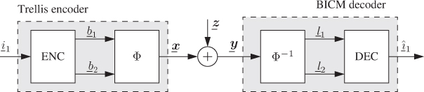
Figure 9.1 BICM-T system under consideration: a trellis encoder and a BICM decoder
When the (nontrivial) interleaver is present (e.g., in BICM-S or BICM-M), the use of a BICM decoder is mandatory as there is no efficient way of implementing the ML rule. Nevertheless, the receiver in Fig. 9.1 uses the BICM decoding rule, even though the interleaver is not present anymore. As we will see later, this in fact gives an advantage over BICM-S. Therefore, the receiver of BICM-T in Fig. 9.1 corresponds to a conventional BICM receiver, where L-values for each bit are computed and then fed to a binary decoder. Here we consider a CENC and a binary decoder based on the Viterbi algorithm.
9.1.1 PDF of the L-values in BICM-T
At each time instant ![]() , two bits
, two bits ![]() and
and ![]() are transmitted using the same symbol
are transmitted using the same symbol ![]() . The two corresponding L-values
. The two corresponding L-values ![]() and
and ![]() are then obtained from the same observation
are then obtained from the same observation ![]() , and thus,
, and thus, ![]() and
and ![]() are dependent. In principle, we might design a decoder, which is aware of the fact that the L-values are not independent in BICM-T. However, this would go against the BICM principle of using a binary decoder operating “blindly” on the L-values and we thus continue to use the BICM decoder, which applies the decision rules defined in Section 6.2.4.
are dependent. In principle, we might design a decoder, which is aware of the fact that the L-values are not independent in BICM-T. However, this would go against the BICM principle of using a binary decoder operating “blindly” on the L-values and we thus continue to use the BICM decoder, which applies the decision rules defined in Section 6.2.4.
In particular, the decoding metric (6.183) for BICM-T is expressed as
where because of the absence of the interleaver ![]() and
and ![]() .
.
The pairwise-error probability (PEP) in (6.188) for the metric in (9.1) is then given by
where
and
indicates that the L-value ![]() contributes to the PEP only for the values of
contributes to the PEP only for the values of ![]() where
where ![]() . Because the channel is memoryless, the metrics in (9.3) for different time instants
. Because the channel is memoryless, the metrics in (9.3) for different time instants ![]() are independent, and thus, without loss of generality, from now on we drop the time index
are independent, and thus, without loss of generality, from now on we drop the time index ![]() .
.
Depending on values of ![]() and
and ![]() , the metric
, the metric ![]() in (9.3) is calculated as specified in Table 9.1. We will now compute the probability density function (PDF) of
in (9.3) is calculated as specified in Table 9.1. We will now compute the probability density function (PDF) of ![]() in (9.3) for the 12 cases in which
in (9.3) for the 12 cases in which ![]() or
or ![]() .
.
We start with the simplest case, i.e., ![]() and
and ![]() . We use the zero-crossing model (ZcM) from Section 5.5.2 to approximate the PDF of the L-values, and thus, we can use the results in Example 5.19 for the cases
. We use the zero-crossing model (ZcM) from Section 5.5.2 to approximate the PDF of the L-values, and thus, we can use the results in Example 5.19 for the cases ![]() and
and ![]() . In particular, from (5.198), we obtain
. In particular, from (5.198), we obtain
and from (5.197) we obtain
where ![]() (see (5.7)).
(see (5.7)).
The expressions (9.5)–(9.7) give the parameters of 8 out of the 12 PDFs. These parameters are shown in Table 9.2 (not highlighted). In what follows, we consider the problem of computing the remaining four PDFs in Table 9.1, i.e., the PDFs ![]() ,
, ![]() ,
, ![]() , and
, and ![]() .
.
Table 9.2 Mean values and variances of the Gaussian approximation for ![]() in Table 9.1. Eight out of the 12 relevant cases follow directly from Example 5.19. The remaining four (highlighted) are given by (9.9)–(9.10). To indicate that the Gaussian distributions correspond to the same
in Table 9.1. Eight out of the 12 relevant cases follow directly from Example 5.19. The remaining four (highlighted) are given by (9.9)–(9.10). To indicate that the Gaussian distributions correspond to the same ![]() , we use circles (for
, we use circles (for ![]() ), stars (for
), stars (for ![]() ), and diamonds (for
), and diamonds (for ![]() )
)
| — | ||||
| — | ||||
| — | ||||
| — |
As shown in Section 5.1.2, the max-log L-values are piece-wise linear functions of ![]() , and thus, the metrics
, and thus, the metrics ![]() in (9.3), being a linear combinations of
in (9.3), being a linear combinations of ![]() and
and ![]() , are also piece-wise linear functions of
, are also piece-wise linear functions of ![]() . In Fig. 9.2, we show
. In Fig. 9.2, we show ![]() in (9.3) for the four possible cases when
in (9.3) for the four possible cases when ![]() . These functions are obtained by linearly combining the piece-wise functions in Fig. 5.10 (see also (5.53) and (5.54)).
. These functions are obtained by linearly combining the piece-wise functions in Fig. 5.10 (see also (5.53) and (5.54)).
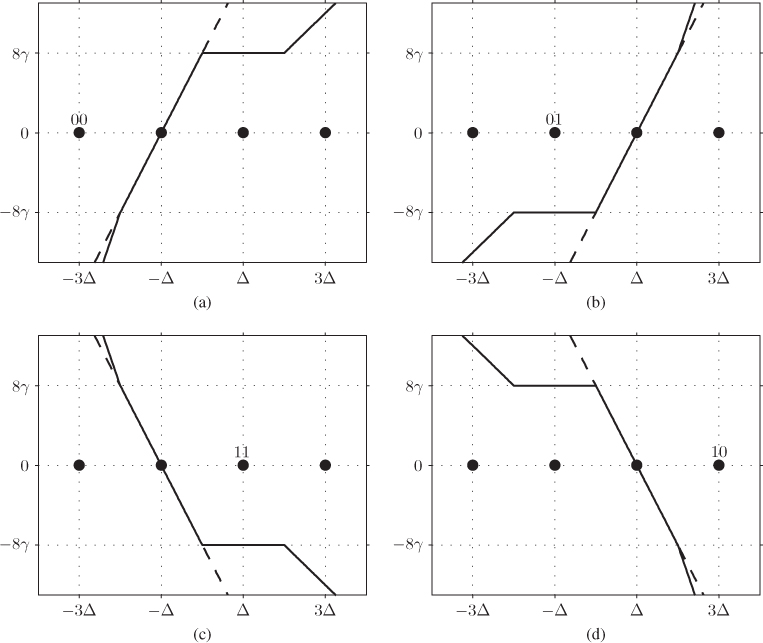
Figure 9.2 Piece-wise relation between the metric  in (9.3) and the received signal
  for all the possible values of
  and
and  , with
  . The four functions (solid lines) are obtained by linearly combining the piece-wise functions in (5.53) and (5.54). The constellation symbols are shown with black circles and the binary labelings of the corresponding symbols relevant for the PDF computation are also shown. The dashed lines represent the linear approximation made by the ZcM approximation. (a)
  ,
,  ; (b)
; (b)  ,
,  ; (c)
; (c)  ,
,  ; and (d)
  ,
, 
For a given transmitted symbol ![]() , the received signal
, the received signal ![]() is a Gaussian random variable with mean
is a Gaussian random variable with mean ![]() and variance
and variance ![]() . Therefore, the PDF of
. Therefore, the PDF of ![]() in (9.3) is a sum of piece-wise truncated Gaussian functions. In order to obtain expressions that are easy to work with, we use again the ZcM, which replaces all the Gaussian pieces by a single Gaussian function. To clarify this, we show in Fig. 9.2 the linear approximation the ZcM does. For example, for
in (9.3) is a sum of piece-wise truncated Gaussian functions. In order to obtain expressions that are easy to work with, we use again the ZcM, which replaces all the Gaussian pieces by a single Gaussian function. To clarify this, we show in Fig. 9.2 the linear approximation the ZcM does. For example, for ![]() (i.e.,
(i.e., ![]() , and
, and ![]() ), we have
), we have
and because ![]() , we obtain
, we obtain
A similar analysis can be done for the remaining three cases, yielding the same result, i.e.,
The parameters of the Gaussian PDFs in (9.9) and (9.10) are the ones we highlight in Table 9.2. This completes the task of finding the 12 densities for the metrics in Table 9.1.
9.1.2 Performance Analysis
Now that we have analytical approximations for the PDF of ![]() in (9.3), we return to the problem of computing the PEP in (9.2). First, from the results in Table 9.2 we see that there are three Gaussian PDFs with different parameters, where the number of Gaussian functions needed to evaluate the PEP in (9.2) depends on the transmitted codeword
in (9.3), we return to the problem of computing the PEP in (9.2). First, from the results in Table 9.2 we see that there are three Gaussian PDFs with different parameters, where the number of Gaussian functions needed to evaluate the PEP in (9.2) depends on the transmitted codeword ![]() and the competing codeword
and the competing codeword ![]() . In principle, this is not a problem, and the PEP can be computed for each possible pair
. In principle, this is not a problem, and the PEP can be computed for each possible pair ![]() . However, the disadvantage of such an approach is that the final PEP expression will have to consider a distance spectrum of the CENC that takes into account all possible pairs of coded sequences that leave a trellis state and remerge after an arbitrary number of trellis stages. In other words, in such a case, the generalized input-dependent weight distribution (GIWD) we considered in Section 8.1.4, which assumes the all-zero codeword was transmitted, cannot be used. This is not surprising as the trellis encoder we consider now is not linear.
. However, the disadvantage of such an approach is that the final PEP expression will have to consider a distance spectrum of the CENC that takes into account all possible pairs of coded sequences that leave a trellis state and remerge after an arbitrary number of trellis stages. In other words, in such a case, the generalized input-dependent weight distribution (GIWD) we considered in Section 8.1.4, which assumes the all-zero codeword was transmitted, cannot be used. This is not surprising as the trellis encoder we consider now is not linear.
To overcome the problem described above, we assume the pseudorandom scrambler in Fig. 3.3 is used. At each time instant ![]() , four scrambler outcomes are possible:
, four scrambler outcomes are possible: ![]() ,
, ![]() ,
, ![]() , and
, and ![]() . For any given pair
. For any given pair ![]() , the distribution of the
, the distribution of the ![]() th metric contribution is given in Table 9.2. It can be shown that for each scrambler outcome, the distribution of the
th metric contribution is given in Table 9.2. It can be shown that for each scrambler outcome, the distribution of the ![]() th metric contribution
th metric contribution ![]() changes over the four distributions shown with the same marker in Table 9.2. For example, for
changes over the four distributions shown with the same marker in Table 9.2. For example, for ![]() and
and ![]() , we see that the
, we see that the ![]() th metric contribution is distributed as
th metric contribution is distributed as ![]() , which is marked with a circle. For
, which is marked with a circle. For ![]() no additional analysis is necessary (the bits are not scrambled), but if
no additional analysis is necessary (the bits are not scrambled), but if ![]() , then
, then ![]() and
and ![]() , and thus, the
, and thus, the ![]() th metric contribution is given by the entry
th metric contribution is given by the entry ![]() in the table (marked with a circle), i.e.,
in the table (marked with a circle), i.e., ![]() . If
. If ![]() the relevant entry in the table is
the relevant entry in the table is ![]() and if
and if ![]() the entry is
the entry is ![]() . The key observation here is that all these four densities (marked with a circle) correspond to the same binary difference
. The key observation here is that all these four densities (marked with a circle) correspond to the same binary difference ![]() . In the case we just described,
. In the case we just described, ![]() .
.
A similar analysis can be done for other cases. For ![]() , all the four distributions marked with a star are covered by changing the scrambler outcome. In this case, the distribution is always given by
, all the four distributions marked with a star are covered by changing the scrambler outcome. In this case, the distribution is always given by ![]() .
.
When ![]() is considered, we have
is considered, we have ![]() , and then, unequal error protection (UEP) effect is apparent: in two out of the four cases the distribution
, and then, unequal error protection (UEP) effect is apparent: in two out of the four cases the distribution ![]() is obtained (low protection), while in the other two cases we obtain the distribution
is obtained (low protection), while in the other two cases we obtain the distribution ![]() (high protection). This means that while scrambler does not affect the distribution for the cases
(high protection). This means that while scrambler does not affect the distribution for the cases ![]() and
and ![]() , it does affect the case
, it does affect the case ![]() .
.
We can summarize the previous discussion by expressing the PDF of the metric in (9.3) (after marginalization over the scrambler outcomes) conditioned on the random variable ![]() modeling the error
modeling the error ![]() , i.e.,
, i.e.,

where
For any linear code, the PEP can then be expressed as
which means that we can assume the all-zero codeword was transmitted and use the PDFs in (9.11)–(9.14) to evaluate the PEP.
To take into account the contribution of the errors ![]() in the PEP, we make a “super-generalization” of the Hamming weight (HW) of
in the PEP, we make a “super-generalization” of the Hamming weight (HW) of ![]() via the vector
via the vector ![]() , where
, where
Then, the PEP in (9.15) can be expressed as
Using the PDF of the L-values in (9.12)–(9.14), we can now calculate the PEP in (9.20). The elements in the integral in (9.20) can be expressed as
where we used ![]() and where the binomial coefficient in (9.21) appears because of the convolution of the sum of the two Gaussian functions in (9.12).
and where the binomial coefficient in (9.21) appears because of the convolution of the sum of the two Gaussian functions in (9.12).
Using the relationships (9.21)–(9.23) in (9.20) yields
where
By using ![]() (see (2.47)) and (9.25) and (9.26) in (9.24), we obtain
(see (2.47)) and (9.25) and (9.26) in (9.24), we obtain

In analogy to (8.22), the bit-error probability (BEP) for BICM-T can be approximated as
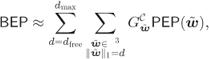
which used with (9.27) gives the final PEP approximation for BICM-T:
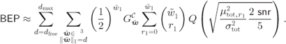
Similarly, an expression for the word-error probability (WEP) for BICM-T can be found, namely,

In (9.29) and (9.30), we use ![]() and
and ![]() , which are the GIWD and generalized weight distribution (GWD) of the CENC. These GIWD and GWD for BICM-T should consider neither the total HW
, which are the GIWD and generalized weight distribution (GWD) of the CENC. These GIWD and GWD for BICM-T should consider neither the total HW ![]() (needed for BICM-S) nor the generalized Hamming weight (GHW)
(needed for BICM-S) nor the generalized Hamming weight (GHW) ![]() (needed for BICM-M), but a GHW
(needed for BICM-M), but a GHW ![]() . In this super-generalization of the HW,
. In this super-generalization of the HW, ![]() counts the number of columns of the divergent sequence in the trellis where
counts the number of columns of the divergent sequence in the trellis where ![]() and
and ![]() ,
, ![]() —the number of columns where
—the number of columns where ![]() and
and ![]() , and
, and ![]() —the number of columns where
—the number of columns where ![]() . In other words, it generalizes the GIWD used in BICM-M in the sense that it considers the case
. In other words, it generalizes the GIWD used in BICM-M in the sense that it considers the case ![]() as a special case. This new GIWD of the encoder is such that for a divergent codeword with HW
as a special case. This new GIWD of the encoder is such that for a divergent codeword with HW ![]() ,
,
The next example shows how to calculate the new, super-generalized ![]() and
and ![]() .
.

Figure 9.3 Generalized state machine for  used in the analysis of BICM-T. The path that generates the FHD event is

Figure 9.4 BEP approximations (lines) and simulation results (markers) for BICM-T, BICM-M, and BICM-S, 4PAM labeled by the BRGC, and for the ODS CENC in Table 2.1:  (
( ) and
) and  (
( ). The BEP approximations are given by (9.29) for BICM-T, by (8.52) for BICM-M, and (6.398) for BICM-S. The asymptotic bounds given by (9.36) are shown with dashed lines
We conclude this section by comparing the results for BICM-T with those obtained for BICM-M and BICM-S. First of all, we note that unlike BICM-M where for ![]() only two variables are needed (
only two variables are needed (![]() and
and ![]() , see Section 8.1.4), in BICM-T three variables are needed (
, see Section 8.1.4), in BICM-T three variables are needed (![]() ,
, ![]() , and
, and ![]() ). If we now consider BICM-S, owing to the interleaver, the case
). If we now consider BICM-S, owing to the interleaver, the case ![]() in (9.11) is ignored because it does not occur frequently (see Fig. 6.13 (a)). In such a case, only circles and diamonds in Table 9.2 should be considered, and thus, only two Gaussian distributions appear in the final density, namely,
in (9.11) is ignored because it does not occur frequently (see Fig. 6.13 (a)). In such a case, only circles and diamonds in Table 9.2 should be considered, and thus, only two Gaussian distributions appear in the final density, namely, ![]() and
and ![]() , with probabilities
, with probabilities ![]() and
and ![]() , respectively. This can also be seen from (9.12) and (9.13) (the PDF in (9.14) is not considered). As expected, this corresponds to the model in Example 6.34, where the probabilities
, respectively. This can also be seen from (9.12) and (9.13) (the PDF in (9.14) is not considered). As expected, this corresponds to the model in Example 6.34, where the probabilities ![]() and
and ![]() correspond to the values of
correspond to the values of ![]() and
and ![]() studied in that example.
studied in that example.
9.2 Code Design for BICM-T
The results from the previous section show relatively large gains offered by BICM-T over BICM-S. In this section, we quantify these gains and we analyze the performance of BICM-T for asymptotically high signal-to-noise ratio (SNR). Asymptotically optimum encoders are defined and BICM-T is also compared with Ungerboeck's TCM.
9.2.1 Asymptotic Bounds
The BEP approximation in (9.29) is a sum of weighted Q-functions, and thus, as ![]() , the BEP is dominated by the Q-functions with the smallest argument. For each
, the BEP is dominated by the Q-functions with the smallest argument. For each ![]() , the dominant Q-function in (9.28) is obtained for
, the dominant Q-function in (9.28) is obtained for ![]() , and thus, the BEP of BICM-T can be (asymptotically) approximated as
, and thus, the BEP of BICM-T can be (asymptotically) approximated as
where
In Fig. 9.4, we show asymptotic approximations for ![]() . For BICM-T we used (9.36), for BICM-S we used (6.399), and for BICM-M we used (8.53). All of them are shown to follow well the simulation results. Similar results can be obtained for the encoder with
. For BICM-T we used (9.36), for BICM-S we used (6.399), and for BICM-M we used (8.53). All of them are shown to follow well the simulation results. Similar results can be obtained for the encoder with ![]() ; however we do not show them so that the figure is not overcrowded.
; however we do not show them so that the figure is not overcrowded.
The asymptotic gain (AG) provided by using BICM-T instead of BICM-S, denoted by ![]() , is obtained directly from (9.36) and (6.399), as stated in the following corollary.
, is obtained directly from (9.36) and (6.399), as stated in the following corollary.
Corollary 9.3 holds for any CENC; however, because ODS CENCs are the asymptotically optimal encoders for BICM-S, studying their loss is of particular interest. To clarify this, consider the following example.
Although the gains offered by BICM-T over BICM-S are quite large, they are bounded, as shown in the following theorem.
The results in Theorem 9.5 are valid for any CENC. In particular, they also hold for the ODS CENCs. As expected, the AG obtained in (9.40) is consistent with (9.43). The AG offered by BICM-T over BICM-S for all the ODS CENCs ![]() (up to
(up to ![]() ) are shown in the eighth column of Table 9.3. The values obtained are around
) are shown in the eighth column of Table 9.3. The values obtained are around ![]() , which is consistent with Theorem 9.5.
, which is consistent with Theorem 9.5.
9.2.2 Optimal Encoders for BICM-T
ODS CENCs are the asymptotically optimal CENCs for binary transmission and for BICM-S, as shown in (6.385). For BICM-M, we showed in Section 8.2.3 that ODS CENCs are not optimal anymore; the optimal joint interleaver and encoder design for BICM-M is given in Definition 8.11. If BICM-T is considered, and as a direct consequence of (9.36), optimal encoders for BICM-T can be defined too. These encoders are asymptotically optimal for BICM-T and guarantee gains for high SNR; however, we will also show that gains appear for low and moderate SNR.
We performed an exhaustive numerical search based on Definition 9.6 and found the optimal encoders for BICM-T. The results are shown in Table 9.3, where for comparison we also show the respective coefficients ![]() and
and ![]() of the ODS CENCs. The search is done in lexicographic order and considering a truncated spectrum
of the ODS CENCs. The search is done in lexicographic order and considering a truncated spectrum ![]() , where
, where ![]() is the FHD of the ODS CENC for that memory
is the FHD of the ODS CENC for that memory ![]() . If there is more than one optimal encoder for a given
. If there is more than one optimal encoder for a given ![]() , we present the first one in the list. As shown in Table 9.3, new encoders (highlighted) are found in four out of six analyzed cases.
, we present the first one in the list. As shown in Table 9.3, new encoders (highlighted) are found in four out of six analyzed cases.
We emphasize that, during the search, the optimal encoders for BICM-T are not assumed to be encoders with MFHD, i.e., ![]() (and not
(and not ![]() ). The results in Table 9.3 confirm this by showing that in general the FHD of the encoder is not the adequate criterion in BICM-T, i.e., encoders with small FHD could perform better than the ODS CENCs (which are obtained by maximizing the FHD, see Section 2.6.1). For example, for
). The results in Table 9.3 confirm this by showing that in general the FHD of the encoder is not the adequate criterion in BICM-T, i.e., encoders with small FHD could perform better than the ODS CENCs (which are obtained by maximizing the FHD, see Section 2.6.1). For example, for ![]() the FHD of the optimal encoder is
the FHD of the optimal encoder is ![]() while for the ODS CENC the FHD is larger (
while for the ODS CENC the FHD is larger (![]() ). The same happens for
). The same happens for ![]() . In fact, only for
. In fact, only for ![]() the ODS CENC is also optimum for BICM-T.3 The results in Table 9.3 also show that the gains offered by the optimal encoders in four out of six cases come from a reduced multiplicity
the ODS CENC is also optimum for BICM-T.3 The results in Table 9.3 also show that the gains offered by the optimal encoders in four out of six cases come from a reduced multiplicity ![]() , i.e., both the optimal and the ODS CENC have the same
, i.e., both the optimal and the ODS CENC have the same ![]() , and thus, the same asymptotic behavior. On the other hand, for
, and thus, the same asymptotic behavior. On the other hand, for ![]() and
and ![]() , there is a differencein
, there is a differencein ![]() that will result in nonzero asymptotic gains. Namely, for
that will result in nonzero asymptotic gains. Namely, for ![]()
and for ![]()
where we used the notation ![]() to show the asymptotic gain of BICM-T using the optimal encoders versus BICM-T using ODS CENCs.
to show the asymptotic gain of BICM-T using the optimal encoders versus BICM-T using ODS CENCs.
9.2.3 BICM-T versus TCM
As explained before, the difference between the system in Fig. 9.1 and TCM is the receiver used. In what follows we compare the asymptotic performance of BICM-T and the optimum ML decoder.
We have previously defined in (9.39) the AG of BICM-T over BICM-S. It is also possible to define the AG of BICM-T compared to uncoded transmission with the same spectral efficiency (uncoded 2PAM). This AG is

which follows from (9.36) and (6.33).
The AG in (9.49) is shown in Table 9.3. For ![]() ,
, ![]() is equal to
is equal to ![]() , which is the same as
, which is the same as ![]() . This is because BICM-S with
. This is because BICM-S with ![]() does not offer any AG compared to uncoded 2PAM.
does not offer any AG compared to uncoded 2PAM.
For comparison, consider the TCM design proposed by Ungerboeck. This is shown in Table 9.4, where the CENCs with their corresponding FHD for different values of ![]() are shown. This table also includes the AG offered by TCM over uncoded transmission with the same spectral efficiency. Analyzing the values of
are shown. This table also includes the AG offered by TCM over uncoded transmission with the same spectral efficiency. Analyzing the values of ![]() in Table 9.3, we find that they are the same as those in Table 9.4. These results show that if BICM-T is used with the correct CENC, it performs asymptotically as well as TCM, and therefore, it should be considered as a good alternative for CM in nonfading channels.4 This is, however, not the case if BICM-S is used, or if BICM-T is used with the ODS CENC. For example, BICM-T for
in Table 9.3, we find that they are the same as those in Table 9.4. These results show that if BICM-T is used with the correct CENC, it performs asymptotically as well as TCM, and therefore, it should be considered as a good alternative for CM in nonfading channels.4 This is, however, not the case if BICM-S is used, or if BICM-T is used with the ODS CENC. For example, BICM-T for ![]() and an ODS CENC gives an AG
and an ODS CENC gives an AG
Table 9.4 Ungerboeck's trellis encoders for ![]() and 4PAM labeled by the natural binary code (NBC) for different
and 4PAM labeled by the natural binary code (NBC) for different ![]()
| 2 | 3 | ||
| 3 | 4 | ||
| 4 | 4 | ||
| 5 | 4 | ||
| 6 | 5 | ||
| 7 | 8 |
which is less than the AG of ![]() offered by BICM-T with an optimal encoder (or by TCM).
offered by BICM-T with an optimal encoder (or by TCM).
For completeness, in Table 9.3, we also show the AG offered by BICM-S over uncoded transmission, defined as ![]() . The performance of uncoded transmission does not depend on
. The performance of uncoded transmission does not depend on ![]() , but increasing
, but increasing ![]() changes the performance of BICM-T and BICM-S. This is reflected in an increase of the asymptotic gains (AGs)
changes the performance of BICM-T and BICM-S. This is reflected in an increase of the asymptotic gains (AGs) ![]() and
and ![]() in Table 9.3 when
in Table 9.3 when ![]() increases. Finally, we also note this is not the case for
increases. Finally, we also note this is not the case for ![]() , where the use of BICM-S with the ODS CENC results in both cases in an asymptotic gain of
, where the use of BICM-S with the ODS CENC results in both cases in an asymptotic gain of ![]() compared to uncoded transmission (see
compared to uncoded transmission (see ![]() in Table 9.3). This can be explained from the fact that the ODS CENCs for
in Table 9.3). This can be explained from the fact that the ODS CENCs for ![]() have the same
have the same ![]() .
.