
CHAPTER 6
Laplace Transforms

Laplace transforms are invaluable for any engineer's mathematical toolbox as they make solving linear ODEs and related initial value problems, as well as systems of linear ODEs, much easier. Applications abound: electrical networks, springs, mixing problems, signal processing, and other areas of engineering and physics.
The process of solving an ODE using the Laplace transform method consists of three steps, shown schematically in Fig. 113:
Step 1. The given ODE is transformed into an algebraic equation, called the subsidiary equation.
Step 2. The subsidiary equation is solved by purely algebraic manipulations.
Step 3. The solution in Step 2 is transformed back, resulting in the solution of the given problem.

Fig. 113. Solving an IVP by Laplace transforms
The key motivation for learning about Laplace transforms is that the process of solving an ODE is simplified to an algebraic problem (and transformations). This type of mathematics that converts problems of calculus to algebraic problems is known as operational calculus. The Laplace transform method has two main advantages over the methods discussed in Chaps. 1–4:
I. Problems are solved more directly: Initial value problems are solved without first determining a general solution. Nonhomogenous ODEs are solved without first solving the corresponding homogeneous ODE.
II. More importantly, the use of the unit step function( Heaviside function in Sec. 6.3) and Dirac's delta (in Sec. 6.4) make the method particularly powerful for problems with inputs (driving forces) that have discontinuities or represent short impulses or complicated periodic functions.
The following chart shows where to find information on the Laplace transform in this book.
| Topic | Where to find it |
| ODEs, engineering applications and Laplace transforms | Chapter 6 |
| PDEs, engineering applications and Laplace transforms | Section 12.11 |
| List of general formulas of Laplace transforms | Section 6.8 |
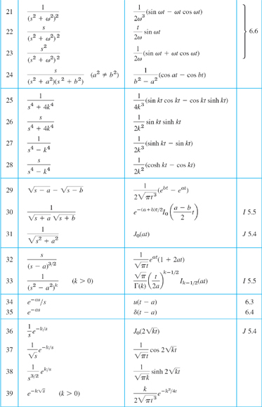
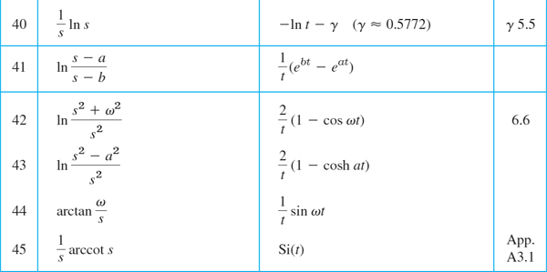
| List of Laplace transforms and inverses | Section 6.9 |
| Note: Your CAS can handle most Laplace transforms. | |
Prerequisite: Chap. 2
Sections that may be omitted in a shorter course: 6.5, 6.7
References and Answers to Problems: App. 1 Part A, App. 2.
6.1 Laplace Transform. Linearity. First Shifting Theorem (s-Shifting)
In this section, we learn about Laplace transforms and some of their properties. Because Laplace transforms are of basic importance to the engineer, the student should pay close attention to the material. Applications to ODEs follow in the next section.
Roughly speaking, the Laplace transform, when applied to a function, changes that function into a new function by using a process that involves integration. Details are as follows.
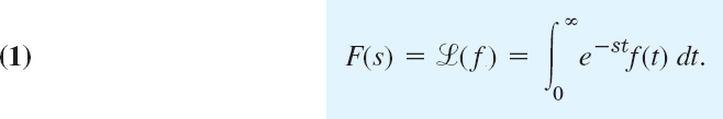
If f(t) is a function defined for all t ![]() 0, its Laplace transform1 is the integral of f(t) times e−st from t = 0 to ∞. It is a function of s, say, F(s), and is denoted by
0, its Laplace transform1 is the integral of f(t) times e−st from t = 0 to ∞. It is a function of s, say, F(s), and is denoted by ![]() (f); thus
(f); thus
Here we must assume that f(t) is such that the integral exists (that is, has some finite value). This assumption is usually satisfied in applications—we shall discuss this near the end of the section.
Not only is the result F(s) called the Laplace transform, but the operation just described, which yields F(s) from a given f(t), is also called the Laplace transform. It is an “integral transform”

with “kernel” k(s, t) = e−st.
Note that the Laplace transform is called an integral transform because it transforms (changes) a function in one space to a function in another space by a process of integration that involves a kernel. The kernel or kernel function is a function of the variables in the two spaces and defines the integral transform.
Furthermore, the given function f(t) in (1) is called the inverse transform of F(s) and is denoted by ![]() −1(F); that is, we shall write
−1(F); that is, we shall write

Note that (1) and (1*) together imply ![]() −1(
−1(![]() (f)) and
(f)) and ![]() (
(![]() −1(F)) = F.
−1(F)) = F.
Notation
Original functions depend on t and their transforms on s—keep this in mind! Original functions are denoted by lowercase letters and their transforms by the same letters in capital, so that F(s) denotes the transform of f(t), and Y(s) denotes the transform of y(t), and so on.
Let f(t) = 1 when t ![]() 0. Find F(s).
0. Find F(s).
Solution. From (1) we obtain by integration

Such an integral is called an improper integral and, by definition, is evaluated according to the rule

Hence our convenient notation means

We shall use this notation throughout this chapter.
EXAMPLE 2 Laplace Transform ![]() (eat) of the Exponential Function) eat
(eat) of the Exponential Function) eat
Let f(t) = eat when t ![]() 0, where a is a constant. Find
0, where a is a constant. Find ![]() (f).
(f).
Solution. Again by (1),

hence, when s − a > 0,
![]()
Must we go on in this fashion and obtain the transform of one function after another directly from the definition? No! We can obtain new transforms from known ones by the use of the many general properties of the Laplace transform. Above all, the Laplace transform is a “linear operation,” just as are differentiation and integration. By this we mean the following.
THEOREM 1 Linearity of the Laplace Transform
The Laplace transform is a linear operation; that is, for any functions f(t) and g(t) whose transforms exist and any constants a and b the transform of af(t) + bg(t) exists, and
![]()
PROOF
This is true because integration is a linear operation so that (1) gives

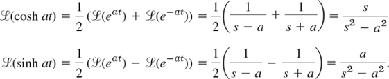
EXAMPLE 3 Application of Theorem 1: Hyperbolic Functions
Find the transforms of cosh at and sinh at.
Solution. Since cosh ![]() and sinh
and sinh ![]() , we obtain from Example 2 and Theorem 1
, we obtain from Example 2 and Theorem 1
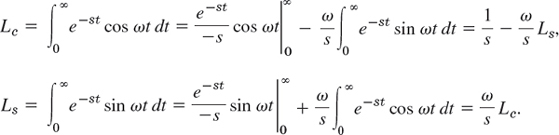
Derive the formulas
![]()
Solution. We write Le = ![]() (cos ωt) and Ls =
(cos ωt) and Ls = ![]() (sin ωt). Integrating by parts and noting that the integral-free parts give no contribution from the upper limit ∞, we obtain
(sin ωt). Integrating by parts and noting that the integral-free parts give no contribution from the upper limit ∞, we obtain
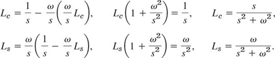
By substituting Ls into the formula for Le on the right and then by substituting Le into the formula for Ls on the right, we obtain
Basic transforms are listed in Table 6.1. We shall see that from these almost all the others can be obtained by the use of the general properties of the Laplace transform. Formulas 1–3 are special cases of formula 4, which is proved by induction. Indeed, it is true for n = 0 because of Example 1 and 0! = 1. We make the induction hypothesis that it holds for any integer n ![]() 0 and then get it for n + 1 directly from (1). Indeed, integration by parts first gives
0 and then get it for n + 1 directly from (1). Indeed, integration by parts first gives
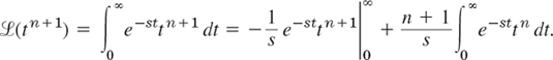
Now the integral-free part is zero and the last part is (n + 1)/s times ![]() (tn). From this and the induction hypothesis,
(tn). From this and the induction hypothesis,

This proves formula 4.
Table 6.1 Some Functions f(t) and Their Laplace Transforms ![]() (f)
(f)

Γ(a + 1) in formula 5 is the so-called gamma function [(15) in Sec. 5.5 or (24) in App. A3.1]. We get formula 5 from (1), setting st = x:
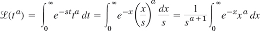
where s > 0. The last integral is precisely that defining Γ(a + 1), so we have Γ(a + 1)/sa+1, as claimed. (CAUTION! Γ(a + 1) has xa in the integral, not xa+1.)
Note the formula 4 also follows from 5 because Γ(n + 1) = n! for integer n ![]() 0.
0.
Formulas 6–10 were proved in Examples 2–4. Formulas 11 and 12 will follow from 7 and 8 by “shifting,” to which we turn next.
s-Shifting: Replacing s by s − a in the Transform
The Laplace transform has the very useful property that, if we know the transform of we can immediately get that of eatf(t), as follows.
THEOREM 2 First Shifting Theorem, s-Shifting
If f (t) has the transform F(s) (where s > k for some k), then eatf(t) has the transform F(s − a) (where s − a > k). In formulas,
![]()
or, if we take the inverse on both sides,
![]()
PROOF
We obtain F(s − a) by replacing s with s − a in the integral in (1), so that
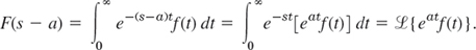
If F(s) exists (i.e., is finite) for s greater than some k, then our first integral exists for s − a > k. Now take the inverse on both sides of this formula to obtain the second formula in the theorem. (CAUTION! −a in F(s − a) but + a in eatf(t).)
EXAMPLE 5 s-Shifting: Damped Vibrations. Completing the Square
From Example 4 and the first shifting theorem we immediately obtain formulas 11 and 12 in Table 6.1,
![]()
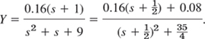
For instance, use these formulas to find the inverse of the transform
![]()
Solution. Applying the inverse transform, using its linearity (Prob. 24), and completing the square, we obtain
![]()
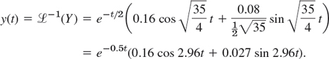
We now see that the inverse of the right side is the damped vibration (Fig. 114)
![]()

Fig. 114. Vibrations in Example 5
Existence and Uniqueness of Laplace Transforms
This is not a big practical problem because in most cases we can check the solution of an ODE without too much trouble. Nevertheless we should be aware of some basic facts.
A function f(t) has a Laplace transform if it does not grow too fast, say, if for all t ![]() 0 and some constants M and k it satisfies the “growth restriction”
0 and some constants M and k it satisfies the “growth restriction”

(The growth restriction (2) is sometimes called “growth of exponential order,” which may be misleading since it hides that the exponent must be kt, not kt2 or similar.)
f(t) need not be continuous, but it should not be too bad. The technical term (generally used in mathematics) is piecewise continuity. f(t) is piecewise continuous on a finite interval a ![]() t
t ![]() b where f is defined, if this interval can be divided into finitely many subintervals in each of which f is continuous and has finite limits as t approaches either endpoint of such a subinterval from the interior. This then gives finite jumps as in Fig. 115 as the only possible discontinuities, but this suffices in most applications, and so does the following theorem.
b where f is defined, if this interval can be divided into finitely many subintervals in each of which f is continuous and has finite limits as t approaches either endpoint of such a subinterval from the interior. This then gives finite jumps as in Fig. 115 as the only possible discontinuities, but this suffices in most applications, and so does the following theorem.

Fig. 115. Example of a piecewise continuous function f(t). (The dots mark the function values at the jumps.)
THEOREM 3 Existence Theorem for Laplace Transforms
If f(t) is defined and piecewise continuous on every finite interval on the semi-axis t ![]() 0 and satisfies (2) for all t
0 and satisfies (2) for all t ![]() 0 and some constants M and k, then the Laplace transform
0 and some constants M and k, then the Laplace transform ![]() (f) exists for all s > k.
(f) exists for all s > k.
PROOF
Since f(t) is piecewise continuous, e−stf(t) is integrable over any finite interval on the t-axis. From (2), assuming that s > k (to be needed for the existence of the last of the following integrals), we obtain the proof of the existence of ![]() (f) from
(f) from
![]()
Note that (2) can be readily checked. For instance, cosh t < et, tn < n!et (because tn/n! is a single term of the Maclaurin series), and so on. A function that does not satisfy (2) for any M and k is ![]() (take logarithms to see it). We mention that the conditions in Theorem 3 are sufficient rather than necessary (see Prob. 22).
(take logarithms to see it). We mention that the conditions in Theorem 3 are sufficient rather than necessary (see Prob. 22).
Uniqueness. If the Laplace transform of a given function exists, it is uniquely determined. Conversely, it can be shown that if two functions (both defined on the positive real axis) have the same transform, these functions cannot differ over an interval of positive length, although they may differ at isolated points (see Ref. [A14] in App. 1). Hence we may say that the inverse of a given transform is essentially unique. In particular, if two continuous functions have the same transform, they are completely identical.
1–16 LAPLACE TRANSFORMS
Find the transform. Show the details of your work. Assume that a, b, ω, θ are constants.
- 3t + 12
- (a − bt)2
- cos πt
- cos2 ωt
- e2t sinh t
- e−t sinh 4t
- sin (ωt + θ)
- 1.5 sin (3t − π/2)


17–24 SOME THEORY
- 17. Table 6.1. Convert this table to a table for finding inverse transforms (with obvious changes, e.g.,
 −1(1/sn) = tn−1/(n − 1), etc).
 - 18. Using (f) in Prob. 10, find (f1) where f1(t) = 0 if t
 2 and f1(t) = 1 if t > 2.
 - 19. Table 6.1. Derive formula 6 from formulas 9 and 10.
- 20. Nonexistence. Show that
 does not satisfy a condition of the form (2).
 - 21. Nonexistence. Give simple examples of functions (defined for all t
 0) that have no Laplace transform.
 - 22. Existence. Show that
 . [Use (30)
  in App. 3.1.] Conclude from this that the conditions in Theorem 3 are sufficient but not necessary for the existence of a Laplace transform.
 - 23. Change of scale. If (f(t)) = F(s) and c is any positive constant, show that (f(ct)) = F(s/c)/c (Hint: Use (1).) Use this to obtain (cos ωt) from (cos t).
- 24. Inverse transform. Prove that −1 is linear. Hint: Use the fact that is linear.
25–32 INVERSE LAPLACE TRANSFORMS
Given F(s) = ![]() (f), find f(t). a, b, L, n are constants. Show the details of your work.
(f), find f(t). a, b, L, n are constants. Show the details of your work.
- 25.

- 26.

- 27.

- 28.

- 29.

- 30.

- 31.

- 32.

33–45 APPLICATION OF s-SHIFTING
In Probs. 33–36 find the transform. In Probs. 37–45 find the inverse transform. Show the details of your work.
- 33. t2e−3t
- 34. ke−at cos ωt
- 35. 0.5e−4.5t sin 2πt
- 36. sinh t cos t
- 37.

- 38.

- 39.

- 40.

- 41.

- 42.

- 43.

- 44.

- 45.

6.2 Transforms of Derivatives and Integrals. ODEs
The Laplace transform is a method of solving ODEs and initial value problems. The crucial idea is that operations of calculus on functions are replaced by operations of algebra on transforms. Roughly, differentiation of f(t) will correspond to multiplication of ![]() (f) by s (see Theorems 1 and 2) and integration of f(t) to division of
(f) by s (see Theorems 1 and 2) and integration of f(t) to division of ![]() (f) by s. To solve ODEs, we must first consider the Laplace transform of derivatives. You have encountered such an idea in your study of logarithms. Under the application of the natural logarithm, a product of numbers becomes a sum of their logarithms, a division of numbers becomes their difference of logarithms (see Appendix 3, formulas (2), (3)). To simplify calculations was one of the main reasons that logarithms were invented in pre-computer times.
(f) by s. To solve ODEs, we must first consider the Laplace transform of derivatives. You have encountered such an idea in your study of logarithms. Under the application of the natural logarithm, a product of numbers becomes a sum of their logarithms, a division of numbers becomes their difference of logarithms (see Appendix 3, formulas (2), (3)). To simplify calculations was one of the main reasons that logarithms were invented in pre-computer times.
THEOREM 1 Laplace Transform of Derivatives
The transforms of the first and second derivatives of f(t) satisfy
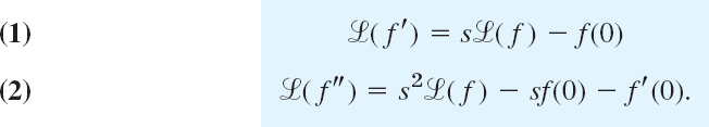
Formula (1) holds if f(t) is continuous for all t ![]() 0 and satisfies the growth restriction (2) in Sec. 6.1 and f′(t) is piecewise continuous on every finite interval on the semi-axis t
0 and satisfies the growth restriction (2) in Sec. 6.1 and f′(t) is piecewise continuous on every finite interval on the semi-axis t ![]() 0. Similarly, (2) holds if f and f′ are continuous for all t
0. Similarly, (2) holds if f and f′ are continuous for all t ![]() 0 and satisfy the growth restriction and f″ is piecewise continuous on every finite interval on the semi-axis t
0 and satisfy the growth restriction and f″ is piecewise continuous on every finite interval on the semi-axis t ![]() 0.
0.
We prove (1) first under the additional assumption that f′ is continuous. Then, by the definition and integration by parts,

Since f satisfies (2) in Sec. 6.1, the integrated part on the right is zero at the upper limit when s > k, and at the lower limit it contributes −f(0). The last integral is ![]() (f). It exists for because of Theorem 3 in Sec. 6.1. Hence
(f). It exists for because of Theorem 3 in Sec. 6.1. Hence ![]() (f′) exists when s > k and (1) holds.
(f′) exists when s > k and (1) holds.
If f′ is merely piecewise continuous, the proof is similar. In this case the interval of integration of f′ must be broken up into parts such that f′ is continuous in each such part.
The proof of (2) now follows by applying (1) to f″ and then substituting (1), that is
![]()
Continuing by substitution as in the proof of (2) and using induction, we obtain the following extension of Theorem 1.
THEOREM 2 Laplace Transform of the Derivative f(n) of Any Order
Let f, f′, …, f(n−1) be continuous for all t ![]() 0 and satisfy the growth restriction (2) in Sec. 6.1. Furthermore, let f(n) be piecewise continuous on every finite interval on the semi-axis t
0 and satisfy the growth restriction (2) in Sec. 6.1. Furthermore, let f(n) be piecewise continuous on every finite interval on the semi-axis t ![]() 0. Then the transform of f(n) satisfies
0. Then the transform of f(n) satisfies
![]()
EXAMPLE 1 Transform of a Resonance Term (Sec. 2.8)
Let f(t) = t sin ωt. Then f(0) = 0, f′(t) = sin ωt + ωt cos ωt, f′(0) = 0, f″ = 2ω cos ωt − ω2t sin ωt. Hence by (2),
![]()
EXAMPLE 2 Formulas 7 and 8 in Table 6.1, Sec. 6.1
This is a third derivation of ![]() (cos ωt) and
(cos ωt) and ![]() (sin ωt); cf. Example 4 in Sec. 6.1. Let f(t) = cos ωt. Then f(0) = 1, f′(0) = 0, f″(t) = −ω2 cos ωt. From this and (2) we obtain
(sin ωt); cf. Example 4 in Sec. 6.1. Let f(t) = cos ωt. Then f(0) = 1, f′(0) = 0, f″(t) = −ω2 cos ωt. From this and (2) we obtain
![]()
Similarly, let g = sin ωt. Then g(0) = 0, g′ = ω cos ωt. From this and (1) we obtain
![]()
Laplace Transform of the Integral of a Function
Differentiation and integration are inverse operations, and so are multiplication and division. Since differentiation of a function f(t) (roughly) corresponds to multiplication of its transform ![]() (f) by s, we expect integration of f(t) to correspond to division of
(f) by s, we expect integration of f(t) to correspond to division of ![]() (f) by s:
(f) by s:
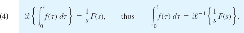
THEOREM 3 Laplace Transform of Integral
Let F(s) denote the transform of a function f(t) which is piecewise continuous for t ![]() 0 and satisfies a growth restriction (2) , Sec.6.1. Then, for s > 0, s > k, and t > 0,
0 and satisfies a growth restriction (2) , Sec.6.1. Then, for s > 0, s > k, and t > 0,
PROOF
Denote the integral in (4) by g(t). Since f(t) is piecewise continuous, g(t) is continuous, and (2), Sec. 6.1, gives

This shows that g(t) also satisfies a growth restriction. Also, g′(t) = f(t), except at points at which f(t) is discontinuous. Hence g′(t) is piecewise continuous on each finite interval and, by Theorem 1, since g(0) = 0 (the integral from 0 to 0 is zero)
![]()
Division by s and interchange of the left and right sides gives the first formula in (4), from which the second follows by taking the inverse transform on both sides.
EXAMPLE 3 Application of Theorem 3: Formulas 19 and 20 in the Table of Sec. 6.9
Using Theorem 3, find the inverse of ![]() .
.
Solution. From Table 6.1 in Sec. 6.1 and the integration in (4) (second formula with the sides interchanged) we obtain
![]()
This is formula 19 in Sec. 6.9. Integrating this result again and using (4) as before, we obtain formula 20 in Sec. 6.9:

It is typical that results such as these can be found in several ways. In this example, try partial fraction reduction.
Differential Equations, Initial Value Problems
Let us now discuss how the Laplace transform method solves ODEs and initial value problems. We consider an initial value problem

where a and b are constant. Here r(t) is the given input (driving force) applied to the mechanical or electrical system and y(t) is the output (response to the input) to be obtained. In Laplace's method we do three steps:
Step 1. Setting up the subsidiary equation. This is an algebraic equation for the transform Y = ![]() (y) obtained by transforming (5) by means of (1) and (2), namely,
(y) obtained by transforming (5) by means of (1) and (2), namely,
![]()
where R(s) = ![]() (r). Collecting the Y-terms, we have the subsidiary equation
(r). Collecting the Y-terms, we have the subsidiary equation
![]()
Step 2. Solution of the subsidiary equation by algebra. We divide by s2 + as + b and use the so-called transfer function
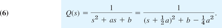
(Q is often denoted by H, but we need H much more frequently for other purposes.) This gives the solution

If y(0) = y′(0) = 0, this is simply y = RQ; hence
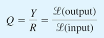
and this explains the name of Q. Note that Q depends neither on r(t) nor on the initial conditions (but only on a and b).
Step 3. Inversion of Y to obtain y = ![]() −1(Y). We reduce (7) (usually by partial fractions as in calculus) to a sum of terms whose inverses can be found from the tables (e.g., in Sec. 6.1 or Sec. 6.9) or by a CAS, so that we obtain the solution y(t) =
−1(Y). We reduce (7) (usually by partial fractions as in calculus) to a sum of terms whose inverses can be found from the tables (e.g., in Sec. 6.1 or Sec. 6.9) or by a CAS, so that we obtain the solution y(t) = ![]() −1(Y) of (5).
−1(Y) of (5).
EXAMPLE 4 Initial Value Problem: The Basic Laplace Steps
Solve
![]()
Solution. Step 1. From (2) and Table 6.1 we get the subsidiary equation [with Y = ![]() (y)]
(y)]
![]()
Step 2. The transfer function is Q = 1/(s2 − 1), and (7) becomes

Simplification of the first fraction and an expansion of the last fraction gives
![]()
Step 3. From this expression for Y and Table 6.1 we obtain the solution
![]()
The diagram in Fig. 116 summarizes our approach.

Fig. 116. Steps of the Laplace transform method
EXAMPLE 5 Comparison with the Usual Method
Solve the initial value problem
![]()
Solution. From (1) and (2) we see that the subsidiary equation is
![]()
The solution is
Hence by the first shifting theorem and the formulas for cos and sin in Table 6.1 we obtain
This agrees with Example 2, Case (III) in Sec. 2.4. The work was less.
Advantages of the Laplace Method
- Solving a nonhomogeneous ODE does not require first solving the homogeneous ODE. See Example 4.
- Initial values are automatically taken care of. See Examples 4 and 5.
- Complicated inputs r(t) (right sides of linear ODEs) can be handled very efficiently, as we show in the next sections.
EXAMPLE 6 Shifted Data Problems
This means initial value problems with initial conditions given at some t = t0 > 0 instead of t = 0. For such a problem set ![]() , so that t = t0 gives
, so that t = t0 gives ![]() and the Laplace transform can be applied. For instance, solve
and the Laplace transform can be applied. For instance, solve
![]()
Solution. We have ![]() and we set
and we set ![]() . Then the problem is
. Then the problem is
![]()
where ![]() . Using (2) and Table 6.1 and denoting the transform of
. Using (2) and Table 6.1 and denoting the transform of ![]() by
by ![]() , we see that the subsidiary equation of the “shifted” initial value problem is
, we see that the subsidiary equation of the “shifted” initial value problem is
![]()
Solving this algebraically for ![]() , we obtain
, we obtain

The inverse of the first two terms can be seen from Example 3 (with ω = 1), and the last two terms give cos and sin,
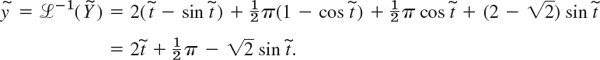
Now ![]() , so that the answer (the solution) is
, so that the answer (the solution) is
![]()
1–11 INITIAL VALUE PROBLEMS (IVPS)
Solve the IVPs by the Laplace transform. If necessary, use partial fraction expansion as in Example 4 of the text. Show all details.
- y′ + 5.2y = 19.4 sin 2t, y(0) = 0
- y′ + 2y = 0, y(0) = 1.5
- y″ − y′ − 6y = 0, y(0) = 11, y′(0) = 28
- y″ + 9y = 10e−t, y(0) = 0, y′(0) = 0

- y″ − 6y′ + 5y = 29 cos 2t, y(0) = 3.2, y′(0) = 6.2
- y″ + 7y′ + 12y = 21e3t, y(0) = 3.5, y′(0) = −10
- y″ − 4y′ + 4y = 0, y(0) = 8.1, y′(0) = 3.9
- y″ − 4y′ + 3y = 6t − 8, y(0) = 0, y′(0) = 0
- y″ + 0.04y = 0.02t2, y(0) = −25, y′(0) = 0
- y″ + 3y′ + 2.25y = 9t3 + 64, y(0) = 1, y′(0) = 31.5
12–15 SHIFTED DATA PROBLEMS
Solve the shifted data IVPs by the Laplace transform. Show the details.
- 12. y″ − 2y′ − 3y = 0, y(4) = −3, y′(4) = −17
- 13. y′ − 6y = 0, y(−1) = 4
- 14. y″ + 2y′ + 5y = 50t − 100, y(2) = −4, y′(2) = 14
- 15. y″ + 3y′ − 4y = 6e2t−3, y(1.5) = 4, y′(1.5) = 5
16–21 OBTAINING TRANSFORMS BY DIFFERENTIATION
Using (1) or (2), find ![]() (f) if f(t) equals:
(f) if f(t) equals:
- 16. t cos 4t
- 17. te−at
- 18. cos22t
- 19. sin2 ωt
- 20. sin4 t. Use Prob. 19.
- 21. cosh2 t
- 22. PROJECT. Further Results by Differentiation. Proceeding as in Example 1, obtain
and from this and Example 1: (b) formula 21, (c) 22, (d) 23 in Sec. 6.9,

23–29 INVERSE TRANSFORMS BY INTEGRATION
Using Theorem 3, find f(t) if ![]() (F) equals:
(F) equals:
- 23.

- 24.

- 25.

- 26.

- 27.

- 28.

- 29.

- 30. PROJECT. Comments on Sec. 6.2. (a) Give reasons why Theorems 1 and 2 are more important than Theorem 3.
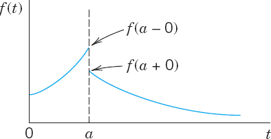
(b) Extend Theorem 1 by showing that if f(t) is continuous, except for an ordinary discontinuity (finite jump) at some t = a (>0), the other conditions remaining as in Theorem 1, then (see Fig. 117)

(c) Verify (1*) for f(t) = e−t if 0 < t < 1 and 0 if t > 1.
(d) Compare the Laplace transform of solving ODEs with the method in Chap. 2. Give examples of your own to illustrate the advantages of the present method (to the extent we have seen them so far).
6.3 Unit Step Function (Heaviside Function). Second Shifting Theorem (t-Shifting)
This section and the next one are extremely important because we shall now reach the point where the Laplace transform method shows its real power in applications and its superiority over the classical approach of Chap. 2. The reason is that we shall introduce two auxiliary functions, the unit step function or Heaviside function u(t − a) (below) and Dirac's delta δ(t − a) (in Sec. 6.4). These functions are suitable for solving ODEs with complicated right sides of considerable engineering interest, such as single waves, inputs (driving forces) that are discontinuous or act for some time only, periodic inputs more general than just cosine and sine, or impulsive forces acting for an instant (hammerblows, for example).
Unit Step Function (Heaviside Function) u(t − a)
The unit step function or Heaviside function u(t − a) is 0 for t < a, has a jump of size 1 at t = a (where we can leave it undefined), and is 1 for t > a, in a formula:
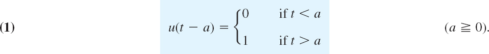

Fig. 118. Unit step function u(t)

Fig. 119. Unit step function u(t − a)
Figure 118 shows the special case u(t) which has its jump at zero, and Fig. 119 the general case u(t − a) for an arbitrary positive a. (For Heaviside, see Sec. 6.1.)
The transform of u(t − a) follows directly from the defining integral in Sec. 6.1,

here the integration begins at t = a (![]() 0) because u(t − a) is 0 for t < a. Hence
0) because u(t − a) is 0 for t < a. Hence

The unit step function is a typical “engineering function” made to measure for engineering applications, which often involve functions (mechanical or electrical driving forces) that are either “off “or “on.” Multiplying functions f(t) with u(t − a), we can produce all sorts of effects. The simple basic idea is illustrated in Figs. 120 and 121. In Fig. 120 the given function is shown in (A). In (B) it is switched off between t = 0 and t = 2 (because u(t − 2) = 0 when t < 2) and is switched on beginning at t = 2. In (C) it is shifted to the right by 2 units, say, for instance, by 2 sec, so that it begins 2 sec later in the same fashion as before. More generally we have the following.
Let f(t) = 0 for all negative t. Then f(t − a)u(t − a) with a > 0 is f(t) shifted (translated) to the right by the amount a.
Figure 121 shows the effect of many unit step functions, three of them in (A) and infinitely many in (B) when continued periodically to the right; this is the effect of a rectifier that clips off the negative half-waves of a sinuosidal voltage. CAUTION! Make sure that you fully understand these figures, in particular the difference between parts (B) and (C) of Fig. 120. Figure 120(C) will be applied next.

Fig. 120. Effects of the unit step function: (A) Given function. (B) Switching off and on. (C) Shift.

Fig. 121. Use of many unit step functions.
Time Shifting (t-Shifting): Replacing t by t − a in f(t)
The first shifting theorem (“s-shifting”) in Sec. 6.1 concerned transforms F(s) = ![]() {f(t)} and F(s − a) =
{f(t)} and F(s − a) = ![]() {eatf(t)}. The second shifting theorem will concern functions f(t) and f(t − a). Unit step functions are just tools, and the theorem will be needed to apply them in connection with any other functions.
{eatf(t)}. The second shifting theorem will concern functions f(t) and f(t − a). Unit step functions are just tools, and the theorem will be needed to apply them in connection with any other functions.
THEOREM 1 Second Shifting Theorem; Time Shifting
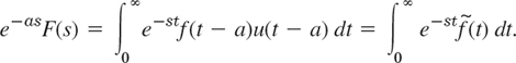
If f(t) has the transform F(s), then the “shifted function”

has the transform e−as F(s). That is, if ![]() {f(t)} = F(s), then
{f(t)} = F(s), then

Or, if we take the inverse on both sides, we can write

Practically speaking, if we know F(s), we can obtain the transform of (3) by multiplying F(s) by e−as. In Fig. 120, the transform of 5 sin t is F(s) = 5/(s2 + 1), hence the shifted function 5 sin (t − 2)u(t − 2) shown in Fig. 120(C) has the transform
![]()
PROOF
We prove Theorem 1. In (4), on the right, we use the definition of the Laplace transform, writing τ for t (to have t available later). Then, taking e−as inside the integral, we have
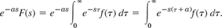
Substituting τ + a = t, thus τ = t − a, dτ = dt in the integral (CAUTION, the lower limit changes!), we obtain
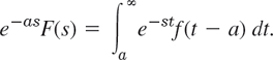
To make the right side into a Laplace transform, we must have an integral from 0 to ∞, not from a to ∞. But this is easy. We multiply the integrand by u(t − a). Then for t from 0 to a the integrand is 0, and we can write, with ![]() as in (3),
as in (3),
(Do you now see why u(t − a) appears?) This integral is the left side of (4), the Laplace transform of ![]() in (3). This completes the proof.
in (3). This completes the proof.
EXAMPLE 1 Application of Theorem 1. Use of Unit Step Functions
Write the following function using unit step functions and find its transform.

Solution. Step 1. In terms of unit step functions,
![]()
Indeed, 2(1 − u(t − 1)) gives f(t) for 0 < t < 1, and so on.
Step 2. To apply Theorem 1, we must write each term in f(t) in the form f(t − a)u(t − a). Thus, 2(1 − u(t − 1)) remains as it is and gives the transform 2(1 − e−s)/s. Then
Together,
![]()
If the conversion of f(t) to f(t − a) is inconvenient, replace it by
![]()
(4**) follows from (4) by writing f(t − a) = g(t), hence f(t) = g(t + a) and then again writing f for g. Thus,
![]()
as before. Similarly for ![]() . Finally, by (4**),
. Finally, by (4**),
![]()
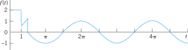
Fig. 122. f(t) in Example 1
EXAMPLE 2 Application of Both Shifting Theorems. Inverse Transform
Find the inverse transform f(t) of

Solution. Without the exponential functions in the numerator the three terms of F(s) would have the inverses (sin πt)/π, (sin πt)/π, and te−2t because 1/s2 has the inverse t, so that 1/(s + 2)2 has the inverse te−2t by the first shifting theorem in Sec. 6.1. Hence by the second shifting theorem (t-shifting),
![]()
Now sin(πt − π) = −sin πt and sin(πt − 2π) = sin πt, so that the first and second terms cancel each other when t > 2. Hence we obtain f(t) = 0 if 0 < t < 1, −(sin πt)/π if 1 < t < 2, 0 if 2 < t < 3, and (t − 3)e−2(t−3) if t < 3. See Fig. 123.

Fig. 123. f(t) in Example 2
EXAMPLE 3 Response of an RC-Circuit to a Single Rectangular Wave
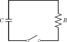
Find the current i(t) in the RC-circuit in Fig. 124 if a single rectangular wave with voltage V0 is applied. The circuit is assumed to be quiescent before the wave is applied.
Solution. The input is V0[u(t − a) − u(t − b)]. Hence the circuit is modeled by the integro-differential equation (see Sec. 2.9 and Fig. 124)
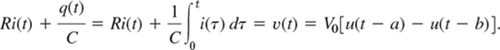
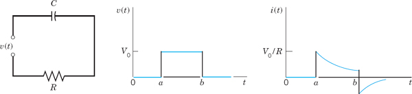
Fig. 124. RC-circuit, electromotive force v(t), and current in Example 3
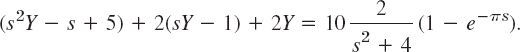
Using Theorem 3 in Sec. 6.2 and formula (1) in this section, we obtain the subsidiary equation
![]()
Solving this equation algebraically for I(s), we get
![]()
the last expression being obtained from Table 6.1 in Sec. 6.1. Hence Theorem 1 yields the solution (Fig. 124)
![]()
that is, i(t) = 0 if t < a, and
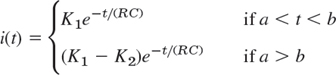
where K1 = V0ea/(RC)/R and K2 = V0eb/(RC)/R.
EXAMPLE 4 Response of an RLC-Circuit to a Sinusoidal Input Acting Over a Time Interval
Find the response (the current) of the RLC-circuit in Fig. 125, where E(t) is sinusoidal, acting for a short time interval only, say,
![]()
and current and charge are initially zero.
Solution. The electromotive force E(t) can be represented by (100 sin 400t)(1 − u(t − 2π)). Hence the model for the current i(t) in the circuit is the integro-differential equation (see Sec. 2.9)

From Theorems 2 and 3 in Sec. 6.2 we obtain the subsidiary equation for I(s) = ![]() (i)
(i)
![]()
Solving it algebraically and noting that s2 + 110s + 1000 = (s + 10)(s + 10)(s + 100), we obtain

For the first term in the parentheses (…) times the factor in front of them we use the partial fraction expansion
![]()
Now determine A, B, D, K by your favorite method or by a CAS or as follows. Multiplication by the common denominator gives
![]()
We set s = −10 and −100 and then equate the sums of the s3 and s2 terms to zero, obtaining (all values rounded)
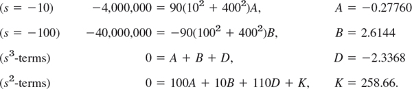
Since K = 258.66 = 0.6467 · 400, we thus obtain for the first term I1 in I = I1 − I2
![]()
From Table 6.1 in Sec. 6.1 we see that its inverse is
![]()
This is the current i(t) when 0 < t < 2π. It agrees for 0 < t < 2π with that in Example 1 of Sec. 2.9 (except for notation), which concerned the same RLC-circuit. Its graph in Fig. 63 in Sec. 2.9 shows that the exponential terms decrease very rapidly. Note that the present amount of work was substantially less.
The second term I1 of I differs from the first term by the factor e−2πs. Since cos 400(t − 2π) = cos 400t and sin 400(t − 2π) = sin 400t, the second shifting theorem (Theorem 1) gives the inverse i2(t) = 0 if 0 < t < 2π, and for > 2π it gives
![]()
Hence in i(t) the cosine and sine terms cancel, and the current for t > 2π is
![]()
It goes to zero very rapidly, practically within 0.5 sec.
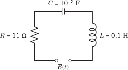
Fig. 125. RLC-circuit in Example 4
- Report on Shifting Theorems. Explain and compare the different roles of the two shifting theorems, using your own formulations and simple examples. Give no proofs.
2–11 SECOND SHIFTING THEOREM, UNIT STEP FUNCTION
Sketch or graph the given function, which is assumed to be zero outside the given interval. Represent it, using unit step functions. Find its transform. Show the details of your work.
- 2. t (0 < t < 2)
- 3. t − 2(t > 2)
- 4. cos 4t(0 < t < π)
- 5. et(0 < t < π/2)
- 6. sin πt(2 < t < 4)
- 7. e−πt (2 < t < 4)
- 8. t2(1 < t < 2)
- 9.

- 10. sinh t (0 < t < 2)
- 11. sin t(π/2 < t < π)
12–17 INVERSE TRANSFORMS BY THE 2ND SHIFTING THEOREM
Find and sketch or graph f(t) if ![]() (f) equals
(f) equals
- 12. e−3s/(s − 1)3
- 13. 6(1 − e−πs)/(s2 + 9)
- 14. 4(e−2s − 2e−5s)/s
- 15. e−3s/s4
- 16. 2(e−s − e−3s)/(s2 − 4)
- 17. (1 + e−2π(s+1))(s + 1)/((s + 1)2 + 1)
18–27 IVPs, SOME WITH DISCONTINUOUS INPUT
Using the Laplace transform and showing the details, solve
- 18. 9y″ − 6y′ + y = 0, y(0) = 3, y′(0) = 1
- 19. y″ + 6y′ + 8y = e−3t − e−5t, y(0) = 0, y′(0) = 0
- 20. y″ + 10y′ + 24y = 144t2, y(0) = 19/12, y′(0) = −5
- 21. y″ + 9y = 8 sin t if 0 < t < π and 0 if t > π; y(0) = 0, y′(0) = 4
- 22. y″ + 3y′ + 2y = 4t if 0 < t < 1 and 8 if t > 1; y(0) = 0, y′(0) = 0
- 23. y″ + y′ − 2y = 3 sin t − cos t if 0 < t < 2π and 3 sin 2t − cos 2t if t > 2π; y(0) = 1, y′(0) = 0
- 24. y″ + 3y′ + 2y = 1 if 0 < t < t and 0 if t > 1; y(0) = 0, y′(0) = 0
- 25. y″ + y = t if 0 < t < 1 and 0 if t > 1; y(0) = 0, y′(0) = 0
- 26. Shifted data. y″ + 2y′ + 5y = 10 sin t if 0 < t < 2π and 0 if t > 2π; y(π) = 1, y′(π) = 2e−π − 2
- 27. Shifted data. y″ + 4y = 8t2 if 0 < t < 5 and 0 if t > 5; y(1) = 1 + cos 2, y′(1) = 4 − 2 sin 2
28–40 MODELS OF ELECTRIC CIRCUITS
28–30 RC-CIRCUIT
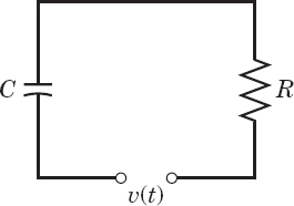
Using the Laplace transform and showing the details, find the current in the circuit i(t) in Fig. 126, assuming i(0) = 0 and:
- 28. R = 1 kΩ (= 1000 Ω), L = 1 H, ν = 0 if 0 < t < π, and 40 sin t V if t > π
- 29. R = 25 Ω, L = 0.1 H, ν = 490 e−5t V if 0 < t < 1 and 0 if t > 1
- 30. R = 10 Ω, L = 0.5 H, ν = 200t V if 0 < t < 2 and 0 if t > 2

- 31. Discharge in RC-circuit. Using the Laplace transform, find the charge q(t) on the capacitor of capacitance C in Fig. 127 if the capacitor is charged so that its potential is V0 and the switch is closed at t = 0.
32–34 RL-CIRCUIT
Using the Laplace transform and showing the details, find the current i(t) in the circuit in Fig. 128 with R = 10 Ω and C = 10−2 F, where the current at t = 0 is assumed to be zero, and:
- 32. ν = 0 if t < 4 and 1.4 · 106e−3t V if t > 4
- 33. ν = 0 if t < 2 and 100(t − 2) V if t > 2
- 34. ν(t) = 100 V if 0.5 < t < 0.6 and 0 otherwise. Why does i(t) have jumps?
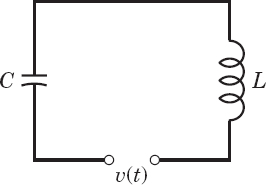
35–37 LC-CIRCUIT
Using the Laplace transform and showing the details, find the current i(t) in the circuit in Fig. 129, assuming zero initial current and charge on the capacitor and:
- 35. L = 1 H, C = 10−2 F, ν = −9900 cos t V if π < t < 3π and 0 otherwise
- 36.
 0 < t < 1 and 0 if t > 1
 - 37. L = 0.5 H, C = 0.05 F, ν = 78 sin t V if 0 < t < π and 0 if t > π
38–40 RLC-CIRCUIT
Using the Laplace transform and showing the details, find the current i(t) in the circuit in Fig. 130, assuming zero initial current and charge and:


6.4 Short Impulses. Dirac's Delta Function. Partial Fractions
An airplane making a “hard” landing, a mechanical system being hit by a hammerblow, a ship being hit by a single high wave, a tennis ball being hit by a racket, and many other similar examples appear in everyday life. They are phenomena of an impulsive nature where actions of forces—mechanical, electrical, etc.—are applied over short intervals of time.
We can model such phenomena and problems by “Dirac's delta function,” and solve them very effecively by the Laplace transform.
To model situations of that type, we consider the function

(and later its limit as k → 0). This function represents, for instance, a force of magnitude 1/k acting from t = a to t = a + k, where k is positive and small. In mechanics, the integral of a force acting over a time interval a ![]() t
t ![]() a + k is called the impulse of the force; similarly for electromotive forces E(t) acting on circuits. Since the blue rectangle in Fig. 132 has area 1, the impulse of fk in (1) is
a + k is called the impulse of the force; similarly for electromotive forces E(t) acting on circuits. Since the blue rectangle in Fig. 132 has area 1, the impulse of fk in (1) is
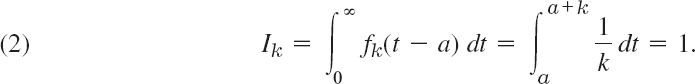

Fig. 132. The function fk(t − a) in (1)
To find out what will happen if k becomes smaller and smaller, we take the limit of fk as k → 0 (k > 0). This limit is denoted by δ(t − a), that is,
![]()
δ(t − a) is called the Dirac delta function2 or the unit impulse function.
δ(t − a) is not a function in the ordinary sense as used in calculus, but a so-called generalized function.2 To see this, we note that the impulse Ik of fk is 1, so that from (1) and (2) by taking the limit as k → 0 we obtain

but from calculus we know that a function which is everywhere 0 except at a single point must have the integral equal to 0. Nevertheless, in impulse problems, it is convenient to operate on δ(t − a) as though it were an ordinary function. In particular, for a continuous function g(t) one uses the property [often called the sifting property of δ(t − a), not to be confused with shifting]
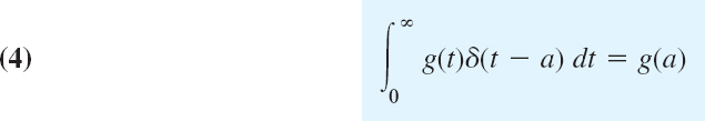
which is plausible by (2).
To obtain the Laplace transform of δ(t − a), we write
![]()
and take the transform [see (2)]
![]()
We now take the limit as k → 0. By l'Hôpital's rule the quotient on the right has the limit 1 (differentiate the numerator and the denominator separately with respect to k, obtaining se−ks and s, respectively, and use se−ks/s → 1 as k → 0). Hence the right side has the limit e−as. This suggests defining the transform of δ(t − a) by this limit, that is,

The unit step and unit impulse functions can now be used on the right side of ODEs modeling mechanical or electrical systems, as we illustrate next.
EXAMPLE 1 Mass–Spring System Under a Square Wave
Determine the response of the damped mass–spring system (see Sec. 2.8) under a square wave, modeled by (see Fig. 133)
![]()
Solution. From (1) and (2) in Sec. 6.2 and (2) and (4) in this section we obtain the subsidiary equation
![]()
Using the notation F(s) and partial fractions, we obtain
From Table 6.1 in Sec. 6.1, we see that the inverse is
![]()
Therefore, by Theorem 1 in Sec. 6.3 (t-shifting) we obtain the square-wave response shown in Fig. 133,

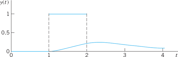
Fig. 133. Square wave and response in Example 1
EXAMPLE 2 Hammerblow Response of a Mass–Spring System
Find the response of the system in Example 1 with the square wave replaced by a unit impulse at time t = 1.
Solution. We now have the ODE and the subsidiary equation
![]()
Solving algebraically gives
![]()
By Theorem 1 the inverse is

y(t) is shown in Fig. 134. Can you imagine how Fig. 133 approaches Fig. 134 as the wave becomes shorter and shorter, the area of the rectangle remaining 1?
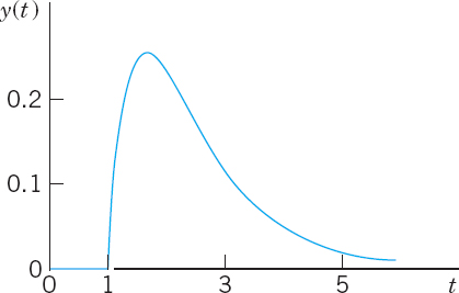
Fig. 134. Response to a hammerblow in Example 2
EXAMPLE 3 Four-Terminal RLC-Network
Find the output voltage response in Fig. 135 if R = 20 Ω, L = 1 H, C = 10−4 F, the input is δ(t)(a unit impulse at time t = 0), and current and charge are zero at time t = 0.
Solution. To understand what is going on, note that the network is an RLC-circuit to which two wires at A and B are attached for recording the voltage v(t) on the capacitor. Recalling from Sec. 2.9 that current i(t) and charge q(t) are related by i = q′ = dq/dt, we obtain the model
![]()
From (1) and (2) in Sec. 6.2 and (5) in this section we obtain the subsidiary equation for Q(s) = ![]() (q)
(q)
![]()
By the first shifting theorem in Sec. 6.1 we obtain from Q damped oscillations for q and v; rounding 9900 ≈ 99.502, we get (Fig. 135)
![]()

Fig. 135. Network and output voltage in Example 3
More on Partial Fractions
We have seen that the solution Y of a subsidiary equation usually appears as a quotient of polynomials Y(s) = F(s)/G(s), so that a partial fraction representation leads to a sum of expressions whose inverses we can obtain from a table, aided by the first shifting theorem (Sec. 6.1). These representations are sometimes called Heaviside expansions.
An unrepeated factor s − a in G(s) requires a single partial fraction A/(s − a). See Examples 1 and 2. Repeated real factors (s − a)2, (s − a)3, etc., require partial fractions
![]()
The inverses are ![]() , etc.
, etc.
Unrepeated complex factors (s − a)(s − ![]() ), a = α + iβ,
), a = α + iβ, ![]() = α − iβ, require a partial fraction (As + B)/[(s − α)2 + β2]. For an application, see Example 4 in Sec. 6.3. A further one is the following.
= α − iβ, require a partial fraction (As + B)/[(s − α)2 + β2]. For an application, see Example 4 in Sec. 6.3. A further one is the following.
EXAMPLE 4 Unrepeated Complex Factors. Damped Forced Vibrations
Solve the initial value problem for a damped mass–spring system acted upon by a sinusoidal force for some time interval (Fig. 136),
![]()
Solution. From Table 6.1, (1), (2) in Sec. 6.2, and the second shifting theorem in Sec. 6.3, we obtain the subsidiary equation
We collect the Y-terms, (s2 + 2s + 2)Y, take to the right, and solve,

For the last fraction we get from Table 6.1 and the first shifting theorem

In the first fraction in (6) we have unrepeated complex roots, hence a partial fraction representation
![]()
Multiplication by the common denominator gives
![]()
We determine A, B, M, N. Equating the coefficients of each power of s on both sides gives the four equations

We can solve this, for instance, obtaining M = −A from (a), then A = B from (c), then N = −3A from (b), and finally A = −2 from (d). Hence a = −2, B = −2, N = 6, and the first fraction in (6) has the representation

The sum of this inverse and (7) is the solution of the problem for 0 < t < π, namely (the sines cancel),
![]()
In the second fraction in (6), taken with the minus sign, we have the factor e−πs so that from (8) and the second shifting theorem (Sec. 6.3) we get the inverse transform of this fraction for t > 0 in the form

The sum of this and (9) is the solution for t > π,
![]()
Figure 136 shows (9) (for 0 < t < π) and (10) (for t > π), a beginning vibration, which goes to zero rapidly because of the damping and the absence of a driving force after t = π.

Fig. 136. Example 4
The case of repeated complex factors [(s − a)(s − ![]() )]2, which is important in connection with resonance, will be handled by “convolution” in the next section.
)]2, which is important in connection with resonance, will be handled by “convolution” in the next section.
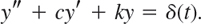
- CAS PROJECT. Effect of Damping. Consider a vibrating system of your choice modeled by
(a) Using graphs of the solution, describe the effect of continuously decreasing the damping to 0, keeping k constant.
(b) What happens if c is kept constant and k is continuously increased, starting from 0?
(c) Extend your results to a system with two δ-functions on the right, acting at different times.
- CAS EXPERIMENT. Limit of a Rectangular Wave. Effects of Impulse.
(a) In Example 1 in the text, take a rectangular wave of area 1 from 1 to 1 + k. Graph the responses for a sequence of values of k approaching zero, illustrating that for smaller and smaller k those curves approach the curve shown in Fig. 134. Hint: If your CAS gives no solution for the differential equation, involving k, take specific k's from the beginning.
(b) Experiment on the response of the ODE in Example 1 (or of another ODE of your choice) to an impulse δ(t − a) for various systematically chosen a (> 0); choose initial conditions y(0) ≠ 0, y′(0) = 0. Also consider the solution if no impulse is applied. Is there a dependence of the response on a? On b if you choose bδ(t − a)? Would −δ(t − ã) with ã > a annihilate the effect of δ(t − a)? Can you think of other questions that one could consider experimentally by inspecting graphs?
3–12 EFFECT OF DELTA (IMPULSE) ON VIBRATING SYSTEMS
Find and graph or sketch the solution of the IVP. Show the details.
- 3. y″ + 4y = δ(t − π), y(0) = 8, y′ (0) = 0
- 4. y″ + 16y = 4δ(t − 3π), y(0) = 2, y′(0) = 0
- 5. y″ + y = δ(t − π) − δ(t − 2π), y(0) = 0, y′(0) = 1
- 6. y″ + 4y′ + 5y = δ(t − 1), y(0) = 0, y′(0) = 3
- 7.
- 8. y″ + 3y′ + 2y = 10(sin t + δ(t − 1)), y(0) = 1, y′(0) = −1
- 9. y″ + 4y′ + 5y = [1 − u(t − 10)]et − e10δ(t − 10)), y(0) = 0, y′(0) = 1
- 10.
- 11. y″ + 5y′ + 6y = u(t − 1) + δ(t − 2), y(0) = 0, y′(0) = 1
- 12. y″ + 2y′ + 5y = 25t − 100δ(t − π), y(0) = −2, y′(0) = 5
- 13. PROJECT. Heaviside Formulas. (a) Show that for a simple root a and fraction A/(s − a) in F(s)/G(s) we have the Heaviside formula

(b) Similarly, show that for a root a of order m and fractions in

we have the Heaviside formulas for the first coefficient

and for the other coefficients

- 14. TEAM PROJECT. Laplace Transform of Periodic Functions
(a) Theorem. The Laplace transform of a piecewise continuous function f(t) with period p is

Prove this theorem. Hint: Write
 .
.Set t = (n − 1)p in the nth integral. Take out e−(n−1)p from under the integral sign. Use the sum formula for the geometric series.
(b) Half-wave rectifier. Using (11), show that the half-wave rectification of sin ωt in Fig. 137 has the Laplace transform

(A half-wave rectifier clips the negative portions of the curve. A full-wave rectifier converts them to positive; see Fig. 138.)
(c) Full-wave rectifier. Show that the Laplace transform of the full-wave rectification of sin ωt is

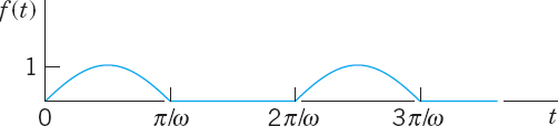
Fig. 137. Half-wave rectification

Fig. 138. Full-wave rectification
(d) Saw-tooth wave. Find the Laplace transform of the saw-tooth wave in Fig. 139.

- 15. Staircase function. Find the Laplace transform of the staircase function in Fig. 140 by noting that it is the difference of kt/p and the function in 14(d).

6.5 Convolution. Integral Equations
Convolution has to do with the multiplication of transforms. The situation is as follows. Addition of transforms provides no problem; we know that ![]() (f + g) =
(f + g) = ![]() (f) +
(f) + ![]() (g). Now multiplication of transforms occurs frequently in connection with ODEs, integral equations, and elsewhere. Then we usually know
(g). Now multiplication of transforms occurs frequently in connection with ODEs, integral equations, and elsewhere. Then we usually know ![]() (f) and
(f) and ![]() (g) and would like to know the function whose transform is the product
(g) and would like to know the function whose transform is the product ![]() (f)
(f)![]() (g). We might perhaps guess that it is fg, but this is false. The transform of a product is generally different from the product of the transforms of the factors,
(g). We might perhaps guess that it is fg, but this is false. The transform of a product is generally different from the product of the transforms of the factors,
![]()
To see this take f = et and g = 1. Then fg = et, ![]() (fg) = 1/(s − 1), but
(fg) = 1/(s − 1), but ![]() (f) = 1/(s − 1) and
(f) = 1/(s − 1) and ![]() (1) = 1/s give
(1) = 1/s give ![]() (f)
(f)![]() (g) = 1/(s2 − s).
(g) = 1/(s2 − s).
According to the next theorem, the correct answer is that ![]() (f)
(f)![]() (g) is the transform of the convolution of f and g, denoted by the standard notation f * g and defined by the integral
(g) is the transform of the convolution of f and g, denoted by the standard notation f * g and defined by the integral

If two functions f and g satisfy the assumption in the existence theorem in Sec. 6.1, so that their transforms F and G exist, the product H = FG is the transform of h given by (1) . (Proof after Example 2.)
Let H(s) = 1/[(s − a)s]. Find h(t).
Solution. 1/(s − a) has the inverse f(t = eat, and 1/s has the inverse g(t) = 1. With f(τ) = eaτ and g(t − τ) ≡ 1 we thus obtain from (1) the answer
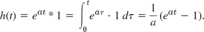
To check, calculate
![]()
Let H(s) = 1/(s2 + ω2)2. Find h(t).
Solution. The inverse of 1/(s2 + ω2 is (sin ωt)/ω. Hence from (1) and the first formula in (11) in App. 3.1 we obtain


in agreement with formula 21 in the table in Sec. 6.9.
PROOF
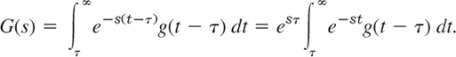
We prove the Convolution Theorem 1. CAUTION! Note which ones are the variables of integration! We can denote them as we want, for instance, by τ and p, and write

We now set t = p + τ, where τ is at first constant. Then p = t − τ, and t varies from τ to ∞. Thus
τ in F and t in G vary independently. Hence we can insert the G-integral into the F-integral. Cancellation of e−sτ and esτ then gives

Here we integrate for fixed τ over t from τ to ∞ and then over τ from 0 to ∞. This is the blue region in Fig. 141. Under the assumption on f and g the order of integration can be reversed (see Ref. [A5] for a proof using uniform convergence). We then integrate first over τ from 0 to t and then over t from 0 to ∞, that is,

This completes the proof.

Fig. 141. Region of integration in the tτ-plane in the proof of Theorem 1
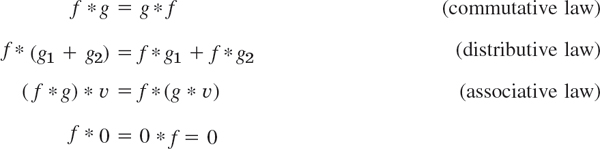
From the definition it follows almost immediately that convolution has the properties
similar to those of the multiplication of numbers. However, there are differences of which you should be aware.
EXAMPLE 3 Unusual Properties of Convolution
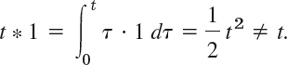
f * 1 ≠ f in general. For instance,
(f * f)(t) ![]() 0 may not hold. For instance, Example 2 with ω = 1 gives
0 may not hold. For instance, Example 2 with ω = 1 gives
![]()
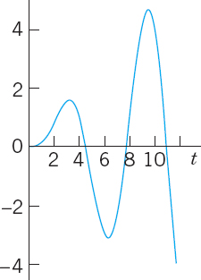
Fig. 142. Example 3
We shall now take up the case of a complex double root (left aside in the last section in connection with partial fractions) and find the solution (the inverse transform) directly by convolution.
EXAMPLE 4 Repeated Complex Factors. Resonance
In an undamped mass–spring system, resonance occurs if the frequency of the driving force equals the natural frequency of the system. Then the model is (see Sec. 2.8)
![]()
where ![]() is the spring constant, and m is the mass of the body attached to the spring. We assume y(0) = 0 and y′(0) = 0, for simplicity. Then the subsidiary equation is
is the spring constant, and m is the mass of the body attached to the spring. We assume y(0) = 0 and y′(0) = 0, for simplicity. Then the subsidiary equation is

This is a transform as in Example 2 with ω = ω0 and multiplied by Kω0. Hence from Example 2 we can see directly that the solution of our problem is
![]()
We see that the first term grows without bound. Clearly, in the case of resonance such a term must occur. (See also a similar kind of solution in Fig. 55 in Sec. 2.8.)
Application to Nonhomogeneous Linear ODEs
Nonhomogeneous linear ODEs can now be solved by a general method based on convolution by which the solution is obtained in the form of an integral. To see this, recall from Sec. 6.2 that the subsidiary equation of the ODE
![]()
has the solution [(7) in Sec. 6.2]
![]()
with R(s) = ![]() (r) and Q(s) = 1/(s2 + as + b) the transfer function. Inversion of the first term […] provides no difficulty; depending on whether
(r) and Q(s) = 1/(s2 + as + b) the transfer function. Inversion of the first term […] provides no difficulty; depending on whether ![]() is positive, zero, or negative, its inverse will be a linear combination of two exponential functions, or of the form (c1 + c2t)e−at/2, or a damped oscillation, respectively. The interesting term is R(s)Q(s) because r(t) can have various forms of practical importance, as we shall see. If y(0) = 0 and y′(0) = 0, then Y = RQ, and the convolution theorem gives the solution
is positive, zero, or negative, its inverse will be a linear combination of two exponential functions, or of the form (c1 + c2t)e−at/2, or a damped oscillation, respectively. The interesting term is R(s)Q(s) because r(t) can have various forms of practical importance, as we shall see. If y(0) = 0 and y′(0) = 0, then Y = RQ, and the convolution theorem gives the solution

EXAMPLE 5 Response of a Damped Vibrating System to a Single Square Wave
Using convolution, determine the response of the damped mass–spring system modeled by
![]()
This system with an input (a driving force) that acts for some time only (Fig. 143) has been solved by partial fraction reduction in Sec. 6.4 (Example 1).
Solution by Convolution. The transfer function and its inverse are

Hence the convolution integral (3) is (except for the limits of integration)

Now comes an important point in handling convolution. r(τ) = 1 if 1 < τ < 2 only. Hence if t < 1, the integral is zero. If 1 < t < 2, we have to integrate from τ = 1 (not 0) to t. This gives (with the first two terms from the upper limit)
![]()
If t > 2, we have to integrate from τ = 1 to 2 (not to t). This gives
![]()
Figure 143 shows the input (the square wave) and the interesting output, which is zero from 0 to 1, then increases, reaches a maximum (near 2.6) after the input has become zero (why?), and finally decreases to zero in a monotone fashion.
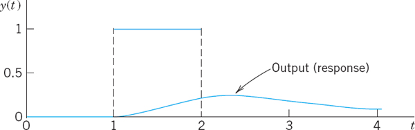
Fig. 143. Square wave and response in Example 5
Integral Equations
Convolution also helps in solving certain integral equations, that is, equations in which the unknown function y(t) appears in an integral (and perhaps also outside of it). This concerns equations with an integral of the form of a convolution. Hence these are special and it suffices to explain the idea in terms of two examples and add a few problems in the problem set.
EXAMPLE 6 A Volterra Integral Equation of the Second Kind
Solve the Volterra integral equation of the second kind3

Solution. From (1) we see that the given equation can be written as a convolution, y − y* sin t = t. Writing Y = ![]() (y) and applying the convolution theorem, we obtain
(y) and applying the convolution theorem, we obtain

The solution is

Check the result by a CAS or by substitution and repeated integration by parts (which will need patience).
EXAMPLE 7 Another Volterra Integral Equation of the Second Kind
Solve the Volterra integral equation
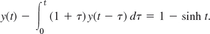
Solution. By (1) we can write y − (1 + t) * y = 1 − sinh t. Writing Y = ![]() (y), we obtain by using the convolution theorem and then taking common denominators
(y), we obtain by using the convolution theorem and then taking common denominators

(s2 − s − 1)/s cancels on both sides, so that solving for Y simply gives
![]()
1–7 CONVOLUTIONS BY INTEGRATION
Find:
- 1 * 1
- 1 * sin ωt
- et * e−t
- (cos ωt) * (cos ωt
- (sin ωt) * (cos ωt)
- eat * ebt(a ≠ b)
- t * et
8–14 INTEGRAL EQUATIONS
Solve by the Laplace transform, showing the details:
- 8.

- 9.

- 10.
- 11.

- 12.
- 13.
- 14.

- 15. CAS EXPERIMENT. Variation of a Parameter.
(a) Replace 2 in Prob. 13 by a parameter k and investigate graphically how the solution curve changes if you vary k, in particular near k = −2.
(b) Make similar experiments with an integral equation of your choice whose solution is oscillating.
- 16. TEAM PROJECT. Properties of Convolution. Prove:
(a) Commutativity, f * g = g * f
(b) Associativity, (f * g) * ν = f * (g * ν)
(c) Distributivity, f * (g1 + g2) = f * g1 + f * g2
(d) Dirac's delta. Derive the sifting formula (4) in Sec. 6.4 by using fk with a = 0 [(1), Sec. 6.4] and applying the mean value theorem for integrals.
(e) Unspecified driving force. Show that forced vibrations governed by

with ω ≠ 0 and an unspecified driving force r(t) can be written in convolution form,
17–26 INVERSE TRANSFORMS BY CONVOLUTION
Showing details, find f(t) if ![]() (f) equals:
(f) equals:
- 17.

- 18.

- 19.

- 20.

- 21.

- 22.

- 23.

- 24.

- 25.

- 26. Partial Fractions. Solve Probs. 17, 21, and 23 by partial fraction reduction.
6.6 Differentiation and Integration of Transforms. ODEs with Variable Coefficients
The variety of methods for obtaining transforms and inverse transforms and their application in solving ODEs is surprisingly large. We have seen that they include direct integration, the use of linearity (Sec. 6.1), shifting (Secs. 6.1, 6.3), convolution (Sec. 6.5), and differentiation and integration of functions f(t) (Sec. 6.2). In this section, we shall consider operations of somewhat lesser importance. They are the differentiation and integration of transforms F(s) and corresponding operations for functions f(t). We show how they are applied to ODEs with variable coefficients.
Differentiation of Transforms
It can be shown that, if a function f(t) satisfies the conditions of the existence theorem in Sec. 6.1, then the derivative F′(s) = dF/ds of the transform F(s) = ![]() (f) can be obtained by differentiating F(s) under the integral sign with respect to s (proof in Ref. [GenRef4] listed in App. 1). Thus, if
(f) can be obtained by differentiating F(s) under the integral sign with respect to s (proof in Ref. [GenRef4] listed in App. 1). Thus, if
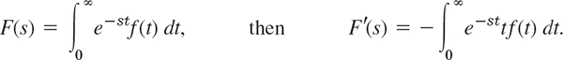
Consequently, if ![]() (f) = F(s), then
(f) = F(s), then

where the second formula is obtained by applying ![]() −1 on both sides of the first formula. In this way, differentiation of the transform of a function corresponds to the multiplication of the function by −t.
−1 on both sides of the first formula. In this way, differentiation of the transform of a function corresponds to the multiplication of the function by −t.
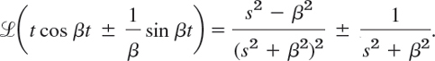
EXAMPLE 1 Differentiation of Transforms. Formulas 21–23 in Sec. 6.9
We shall derive the following three formulas.

Solution. From (1) and formula 8 (with ω = β) in Table 6.1 of Sec. 6.1 we obtain by differentiation (CAUTION! Chain rule!)

Dividing by 2β and using the linearity of ![]() , we obtain (3).
, we obtain (3).
Formulas (2) and (4) are obtained as follows. From (1) and formula 7 (with ω = β) in Table 6.1 we find

From this and formula 8 (with ω = β) in Table 6.1 we have
On the right we now take the common denominator. Then we see that for the plus sign the numerator becomes s2 − β2 + s2 + β2 = 2s2, so that (4) follows by division by 2. Similarly, for the minus sign the numerator takes the form s2 − β2 − s2 − β2 = −2β2, and we obtain (2). This agrees with Example 2 in Sec. 6.5.
Integration of Transforms
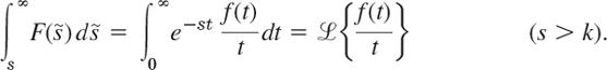
Similarly, if f(t) satisfies the conditions of the existence theorem in Sec. 6.1 and the limit of f(t)/t, as t approaches 0 from the right, exists, then for s > k,
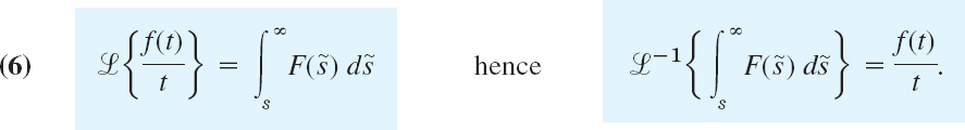
In this way, integration of the transform of a function f(t) corresponds to the division of f(t) by t.
We indicate how (6) is obtained. From the definition it follows that

and it can be shown (see Ref. [GenRef4] in App. 1) that under the above assumptions we may reverse the order of integration, that is,
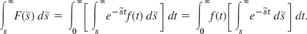
Integration of ![]() with respect to
with respect to ![]() gives
gives ![]() /(−t). Here the integral over
/(−t). Here the integral over ![]() on the right equals e−st/t. Therefore,
on the right equals e−st/t. Therefore,
EXAMPLE 2 Differentiation and Integration of Transforms
Find the inverse transform of ![]() .
.
Solution. Denote the given transform by F(s). Its derivative is

Taking the inverse transform and using (1), we obtain

Hence the inverse f(t) of F(s) is f(t) = 2(1 − cos ωt)/t. This agrees with formula 42 in Sec. 6.9.
Alternatively, if we let
![]()
From this and (6) we get, in agreement with the answer just obtained,

the minus occurring since s is the lower limit of integration.
In a similar way we obtain formula 43 in Sec. 6.9,

Special Linear ODEs with Variable Coefficients
Formula (1) can be used to solve certain ODEs with variable coefficients. The idea is this. Let ![]() (y) = Y. Then
(y) = Y. Then ![]() (y′) = sY − y(0) (see Sec. 6.2). Hence by (1),
(y′) = sY − y(0) (see Sec. 6.2). Hence by (1),

Similarly, ![]() (y″) = s2Y − sy(0) − y′(0) and by (1)
(y″) = s2Y − sy(0) − y′(0) and by (1)

Hence if an ODE has coefficients such as at + b, the subsidiary equation is a first-order ODE for Y, which is sometimes simpler than the given second-order ODE. But if the latter has coefficients at2 + bt + c, then two applications of (1) would give a second-order ODE for Y, and this shows that the present method works well only for rather special ODEs with variable coefficients. An important ODE for which the method is advantageous is the following.
EXAMPLE 3 Laguerre's Equation. Laguerre Polynomials
Laguerre's ODE is

We determine a solution of (9) with n = 0, 1, 2, …. From (7)–(9) we get the subsidiary equation


Separating variables, using partial fractions, integrating (with the constant of integration taken to be zero), and taking exponentials, we get

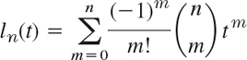
We write ln = ![]() −1(Y) and prove Rodrigues's formula
−1(Y) and prove Rodrigues's formula

These are polynomials because the exponential terms cancel if we perform the indicated differentiations. They are called Laguerre polynomials and are usually denoted by Ln (see Problem Set 5.7, but we continue to reserve capital letters for transforms). We prove (10). By Table 6.1 and the first shifting theorem (s-shifting),

because the derivatives up to the order n − 1 are zero at 0. Now make another shift and divide by n! to get [see (10) and then (10*)]

- REVIEW REPORT. Differentiation and Integration of Functions and Transforms. Make a draft of these four operations from memory. Then compare your draft with the text and write a 2- to 3-page report on these operations and their significance in applications.
2–11 TRANSFORMS BY DIFFERENTIATION
Showing the details of your work, find ![]() (f) if f(t) equals:
(f) if f(t) equals:
- 2. 3t sinh 4t
- 3.

- 4. te−t cos t
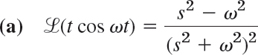
- 5. t cos ωt
- 6. t2 sin 3t
- 7. t2 cosh 2t
- 8. te−kt sin t
- 9.

- 10. tnekt
- 11.

- 12. CAS PROJECT. Laguerre Polynomials. (a) Write a CAS program for finding ln(t) in explicit form from (10). Apply it to calculate l0, …, l10. Verify that l0, …, l10 satisfy Laguerre's differential equation (9).
(b) Show that
and calculate l0, …, l10 from this formula.
(c) Calculate l0, …, l10 recursively from l0 = 1, l1 = 1 − t by

(d) A generating function (definition in Problem Set 5.2) for the Laguerre polynomials is

Obtain l0, …, l10 from the corresponding partial sum of this power series in x and compare the ln with those in (a), (b), or (c).
- 13. CAS EXPERIMENT. Laguerre Polynomials. Experiment with the graphs of l0, …, l10, finding out empirically how the first maximum, first minimum, … is moving with respect to its location as a function of n. Write a short report on this.
Using differentiation, integration, s-shifting, or convolution, and showing the details, find f(t) if ![]() (f) equals:
(f) equals:
- 14.

- 15.

- 16.

- 17.

- 18.

- 19.

- 20.

6.7 Systems of ODEs
The Laplace transform method may also be used for solving systems of ODEs, as we shall explain in terms of typical applications. We consider a first-order linear system with constant coefficients (as discussed in Sec. 4.1)

Writing Y1 = ![]() (y1), Y2 =
(y1), Y2 = ![]() (y2), G1 =
(y2), G1 = ![]() (g1), G2 =
(g1), G2 = ![]() (g2), we obtain from (1) in Sec. 6.2 the subsidiary system
(g2), we obtain from (1) in Sec. 6.2 the subsidiary system

By collecting the Y1- and Y2-terms we have

By solving this system algebraically for Y1(s), Y2(s) and taking the inverse transform we obtain the solution y1 = ![]() −1(Y1), y2 =
−1(Y1), y2 = ![]() −1(Y2) of the given system (1).
−1(Y2) of the given system (1).
Note that (1) and (2) may be written in vector form (and similarly for the systems in the examples); thus, setting y = [y1 y2]T, A = [ajk], g = [g1 g2]T, Y = [Y1 Y2]T, G = [G1 G2]T we have
![]()
EXAMPLE 1 Mixing Problem Involving Two Tanks
Tank T1 in Fig. 144 initially contains 100 gal of pure water. Tank T2 initially contains 100 gal of water in which 150 lb of salt are dissolved. The inflow into T1 is 2 gal/min from T2 and 6 gal/min containing 6 lb of salf from the outside. The inflow into T2 is 8 gal/min from T1. The outflow from T2 is 2 + 6 = 8 gal/min, as shown in the figure. The mixtures are kept uniform by stirring. Find and plot the salt contents y1(t) and y2(t) in T1 and T2 respectively.
Solution. The model is obtained in the form of two equations
![]()
for the two tanks (see Sec. 4.1). Thus,
![]()
The initial conditions are y1(0) = 0, y2(0) = 150. From this we see that the subsidiary system (2) is
We solve this algebraically for Y1 and Y2 by elimination (or by Cramer's rule in Sec. 7.7), and we write the solutions in terms of partial fractions,
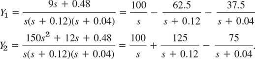
By taking the inverse transform we arrive at the solution

Figure 144 shows the interesting plot of these functions. Can you give physical explanations for their main features? Why do they have the limit 100? Why is y2 not monotone, whereas y1 is? Why is y1 from some time on suddenly larger than y2? Etc.
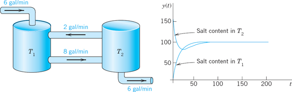
Fig. 144. Mixing problem in Example 1
Other systems of ODEs of practical importance can be solved by the Laplace transform method in a similar way, and eigenvalues and eigenvectors, as we had to determine them in Chap. 4, will come out automatically, as we have seen in Example 1.
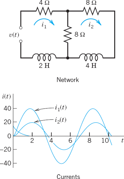
Find the currents i1(t) and i2(t) in the network in Fig. 145 with L and R measured in terms of the usual units (see Sec. 2.9), ν(t) = 100 volts if 0 ![]() t
t ![]() 0.5 sec and 0 thereafter, and i(0) = 0, i′(0) = 0.
0.5 sec and 0 thereafter, and i(0) = 0, i′(0) = 0.
Solution. The model of the network is obtained from Kirchhoff's Voltage Law as in Sec. 2.9. For the lower circuit we obtain
![]()

Fig. 145. Electrical network in Example 2
and for the upper
![]()
Division by 0.8 and ordering gives for the lower circuit
![]()
and for the upper
![]()
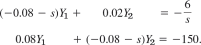
With i1(0) = 0, i2(0) = 0 we obtain from (1) in Sec. 6.2 and the second shifting theorem the subsidiary system

Solving algebraically for I1 and I2 gives

The right sides, without the factor 1 − e−s/2, have the partial fraction expansions
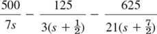
and
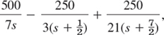
respectively. The inverse transform of this gives the solution for ![]() ,
,
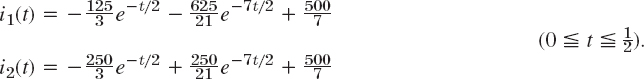
According to the second shifting theorem the solution for ![]() , that is,
, that is,
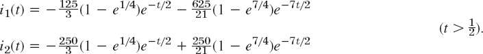
Can you explain physically why both currents eventually go to zero, and why i1(t) has a sharp cusp whereas i2(t) has a continuous tangent direction at ![]() ?
?
Systems of ODEs of higher order can be solved by the Laplace transform method in a similar fashion. As an important application, typical of many similar mechanical systems, we consider coupled vibrating masses on springs.

Fig. 146. Example 3
EXAMPLE 3 Model of Two Masses on Springs (Fig. 146)
The mechanical system in Fig. 146 consists of two bodies of mass 1 on three springs of the same spring constant k and of negligibly small masses of the springs. Also damping is assumed to be practically zero. Then the model of the physical system is the system of ODEs

Here y1 and y2 are the displacements of the bodies from their positions of static equilibrium. These ODEs follow from Newton's second law, Mass × Acceleration = Force, as in Sec. 2.4 for a single body. We again regard downward forces as positive and upward as negative. On the upper body, −ky1 is the force of the upper spring and k(y2 − y1) that of the middle spring, y2 − y1 being the net change in spring length—think this over before going on. On the lower body, −k(y2 − y1) is the force of the middle spring and −ky2 that of the lower spring.
We shall determine the solution corresponding to the initial conditions y1(0) = 1, y2(0) = 1, ![]() ,
, ![]() . Let Y1 =
. Let Y1 = ![]() (y1) and Y2 =
(y1) and Y2 = ![]() (y2). Then from (2) in Sec. 6.2 and the initial conditions we obtain the subsidiary system
(y2). Then from (2) in Sec. 6.2 and the initial conditions we obtain the subsidiary system

This system of linear algebraic equations in the unknowns Y1 and Y2 may be written

Elimination (or Cramer's rule in Sec. 7.7) yields the solution, which we can expand in terms of partial fractions,
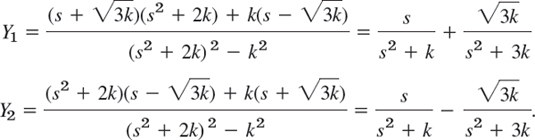
Hence the solution of our initial value problem is (Fig. 147)

We see that the motion of each mass is harmonic (the system is undamped!), being the superposition of a “slow” oscillation and a “rapid” oscillation.

Fig. 147. Solutions in Example 3
- TEAM PROJECT. Comparison of Methods for Linear Systems of ODEs
(a) Models. Solve the models in Examples 1 and 2 of Sec. 4.1 by Laplace transforms and compare the amount of work with that in Sec. 4.1. Show the details of your work.
(b) Homogeneous Systems. Solve the systems (8), (11)–(13) in Sec. 4.3 by Laplace transforms. Show the details.
(c) Nonhomogeneous System. Solve the system (3) in Sec. 4.6 by Laplace transforms. Show the details.
2–15 SYSTEMS OF ODES
Using the Laplace transform and showing the details of your work, solve the IVP:
- 2. y′1 + y2 = 0, y1 + y′2 = 2 cos t, y1(0) = 1, y2(0) = 0
- 3. y′1 = −y1 + 4y2, y′2 = 3y1 − 2y2, y1(0) = 3, y2(0) = 4
- 4. y′1 = 4y2 − 8 cos 4t, y′2 = −3y1 − 9 sin 4t, y1(0) = 0, y2(0) = 3
- 5. y′1 = y2 + 1 − u(t − 1), y′2 = −y1 + 1 − u(t − 1), y1(0) = 0, y2(0) = 0
- 6. y′1 = 5y1 + y2, y′2 = y1 + 5y2, y1(0) = 1, y2(0) = −3
- 7. y′1 = 2y1 − 4y2 + u(t − 1)et,
y′2 = y1 − 3y2 + u(t − 1)et, y1(0) = 3, y2(0) = 0
- 8. y′1 = −2y1 + 3y2, y′2 = 4y1 − y2, y1(0) = 4, y2(0) = 3
- 9. y′1 = 4y1 + y2, y′2 = −y1 + 2y2, y1(0) = 3, y2(0) = 1
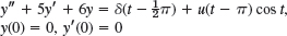
- 10. y′1 = −y2, y′2 = −y1 + 2[1 − u(t − 2π)] cos t, y1(0) = 1, y2(0) = 0
- 11. y″1 = y1 + 3y2, y″2 = 4y1 − 4et, y1(0) = 2, y′1(0) = 3, y2(0) = 1, y′2(0) = 2
- 12. y″1 = −2y1 + 2y2, y″2 = 2y1 − 5y2, y1(0) = 1, y′1(0) = 0, y2(0) = 3, y′2(0) = 0
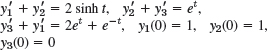
- 13. y″1 + y2 = −101 sin 10t, y″2 + y1 = 101 sin 10t, y1(0) = 0, y′1(0) = 6, y2(0) = 8, y′2(0) = −6
- 14.

- 15.
FURTHER APPLICATIONS
- 16. Forced vibrations of two masses. Solve the model in Example 3 with k = 4 and initial conditions y1(0) = 1, y′1(0) = 1, y2(0) = 1, y′2 = −1 under the assumption that the force 11 sin t is acting on the first body and the force −11 sin t on the second. Graph the two curves on common axes and explain the motion physically.
- 17. CAS Experiment. Effect of Initial Conditions. In Prob. 16, vary the initial conditions systematically, describe and explain the graphs physically. The great variety of curves will surprise you. Are they always periodic? Can you find empirical laws for the changes in terms of continuous changes of those conditions?
- 18. Mixing problem. What will happen in Example 1 if you double all flows (in particular, an increase to containing 12 lb of salt from the outside), leaving the size of the tanks and the initial conditions as before? First guess, then calculate. Can you relate the new solution to the old one?
- 19. Electrical network. Using Laplace transforms, find the currents i1(t) and i2(t) in Fig. 148, where ν(t) = 390 cos t and i1(0) = 0, i2(0) = 0. How soon will the currents practically reach their steady state?
- 20. Single cosine wave. Solve Prob. 19 when the EMF (electromotive force) is acting from 0 to 2π only. Can you do this just by looking at Prob. 19, practically without calculation?
6.8 Laplace Transform: General Formulas
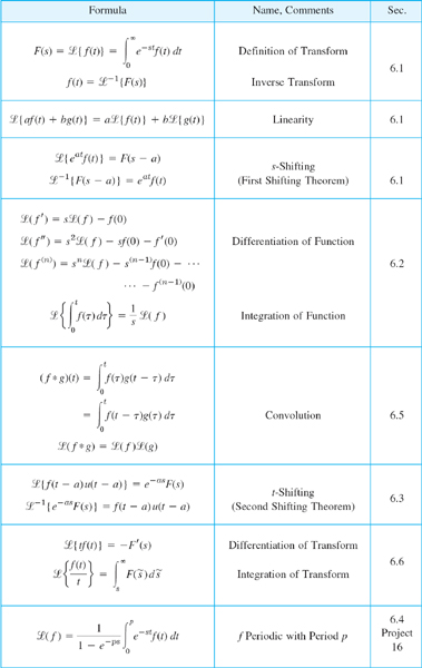
6.9 Table of Laplace Transforms
For more extensive tables, see Ref. [A9] in Appendix 1.

CHAPTER 6 REVIEW QUESTIONS AND PROBLEMS
- State the Laplace transforms of a few simple functions from memory.
- What are the steps of solving an ODE by the Laplace transform?
- In what cases of solving ODEs is the present method preferable to that in Chap. 2?
- What property of the Laplace transform is crucial in solving ODEs?
- Is {f(t) + g(t)} = {f(t)} + {g(t)}? {f(t)g(t)} = {f(t){g(t)}? Explain.
- When and how do you use the unit step function and Dirac's delta?
- If you know f(t) = −1{F(s)}, how would you find −1{F(s)/s2}?
- Explain the use of the two shifting theorems from memory.
- Can a discontinuous function have a Laplace transform? Give reason.
- If two different continuous functions have transforms, the latter are different. Why is this practically important?
11–19 LAPLACE TRANSFORMS
Find the transform, indicating the method used and showing the details.
- 11. 5 cosh 2t − 3 sinh t
- 12. e−t(cos 4t − 2 sin 4t)
- 13.

- 14.

- 15. et/2u(t − 3)
- 16. u(t − 2π) sin t
- 17. t cos t + sin t
- 18. (sin ωt) * (cos ωt)
- 19. 12t * e−3t
20–28 INVERSE LAPLACE TRANSFORM
Find the inverse transform, indicating the method used and showing the details:
- 20.

- 21.

- 22.

- 23.

- 24.

- 25.

- 26.

- 27.

- 28.

29–37 ODEs AND SYSTEMS
Solve by the Laplace transform, showing the details and graphing the solution:
- 29. y″ + 4y′ + 5y = 50t, y(0) = 5, y′(0) = −5
- 30. y″ + 16y = 4δ(t − π), y(0) = −1, y′(0) = 0
- 31. y″ − y′ − 2y = 12u(t − π) sin t, y(0) = 1, y′(0) = −1
- 32. y″ + 4y = δ(t − π) − δ(t − 2π), y(0) = 1, y′(0) = 0
- 33. y″ + 3y′ + 2y = 2u(t − 2), y(0) = 0, y′(0) = 0
- 34. y′1 = y2, y′2 = −4y1 + δ(t − π), y1(0) = 0, y2(0) = 0
- 35. y′1 = 2y1 − 4y2, y′2 = y1 − 3y2, y1(0) = 3, y2(0) = 0
- 36. y′1 = 2y1 + 4y2, y′2 = y1 + 2y2, y1(0) = −4, y2(0) = −4
- 37. y′1 = y2 + u(t − π), y′2 = −y1 + u(t − 2π), y1(0) = 1, y2(0) = 0
38–45 MASS–SPRING SYSTEMS, CIRCUITS, NETWORKS
Model and solve by the Laplace transform:
- 38. Show that the model of the mechanical system in Fig. 149 (no friction, no damping) is
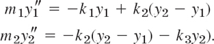

- 39. In Prob. 38, let m1 = m2 = 10 kg, k1 = k3 = 20 kg/sec2, k2 = 40 kg/sec2. Find the solution satisfying the initial conditions y1(0) = y2(0) = 0, y′1(0) = 1 meter/sec, y′2(0) = −1 meter/sec.
- 40. Find the model (the system of ODEs) in Prob. 38 extended by adding another mass and another spring of modulus k4 in series.
- 41. Find the current i(t) in the RC-circuit in Fig. 150, where R = 10 Ω, C = 0.1 F, ν(t) = 10t V if 0 < t < 4, ν(t) = 40 V if t > 4, and the initial charge on the capacitor is 0.

- 42. Find and graph the charge q(t) and the current i(t) in the LC-circuit in Fig. 151, assuming L = 1 H, C = 1 F, ν(t) = 1 − e−t if 0 < t < π, ν(t) = 0 if t > π, and zero initial current and charge.
- 43. Find the current i(t) in the RLC-circuit in Fig. 152, where R = 160 Ω, L = 20 H, C = 0.002 F, ν(t) = 37 sin 10t V, and current and charge at t = 0 are zero.


- 44. Show that, by Kirchhoff's Voltage Law (Sec. 2.9), the currents in the network in Fig. 153 are obtained from the system

Solve this system, assuming that, R = 10 Ω L = 20 H, C = 0.05 F, ν = 20 V, i1(0) = 0, i2(0) = 2 A.

- 45. Set up the model of the network in Fig. 154 and find the solution, assuming that all charges and currents are 0 when the switch is closed at t = 0. Find the limits of i1(t) and i2(t) as t → ∞, (i) from the solution, (ii) directly from the given network.
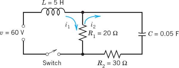
SUMMARY OF CHAPTER 6 Laplace Transforms
The main purpose of Laplace transforms is the solution of differential equations and systems of such equations, as well as corresponding initial value problems. The Laplace transform F(s) = ![]() (f) of a function f(t) is defined by
(f) of a function f(t) is defined by

This definition is motivated by the property that the differentiation of f with respect to t corresponds to the multiplication of the transform F by s; more precisely,

etc. Hence by taking the transform of a given differential equation
![]()
and writing ![]() (y) = Y(s) we obtain the subsidiary equation
(y) = Y(s) we obtain the subsidiary equation
![]()
Here, in obtaining the transform ![]() (r) we can get help from the small table in Sec. 6.1 or the larger table in Sec. 6.9. This is the first step. In the second step we solve the subsidiary equation algebraically for Y(s). In the third step we determine the inverse transform y(t) =
(r) we can get help from the small table in Sec. 6.1 or the larger table in Sec. 6.9. This is the first step. In the second step we solve the subsidiary equation algebraically for Y(s). In the third step we determine the inverse transform y(t) = ![]() −1(Y), that is, the solution of the problem. This is generally the hardest step, and in it we may again use one of those two tables. Y(s) will often be a rational function, so that we can obtain the inverse
−1(Y), that is, the solution of the problem. This is generally the hardest step, and in it we may again use one of those two tables. Y(s) will often be a rational function, so that we can obtain the inverse ![]() −1(Y) by partial fraction reduction (Sec. 6.4) if we see no simpler way.
−1(Y) by partial fraction reduction (Sec. 6.4) if we see no simpler way.
The Laplace method avoids the determination of a general solution of the homogeneous ODE, and we also need not determine values of arbitrary constants in a general solution from initial conditions; instead, we can insert the latter directly into (4). Two further facts account for the practical importance of the Laplace transform. First, it has some basic properties and resulting techniques that simplify the determination of transforms and inverses. The most important of these properties are listed in Sec. 6.8, together with references to the corresponding sections. More on the use of unit step functions and Dirac's delta can be found in Secs. 6.3 and 6.4, and more on convolution in Sec. 6.5. Second, due to these properties, the present method is particularly suitable for handling right sides given by different expressions over different intervals of time, for instance, when is a square wave or an impulse or of a form such as r(t) = cos t if 0 ![]() t
t ![]() 4π and 0 elsewhere.
4π and 0 elsewhere.
The application of the Laplace transform to systems of ODEs is shown in Sec. 6.7. (The application to PDEs follows in Sec. 12.12.)
1 PIERRE SIMON MARQUIS DE LAPLACE (1749–1827), great French mathematician, was a professor in Paris. He developed the foundation of potential theory and made important contributions to celestial mechanics, astronomy in general, special functions, and probability theory. Napoléon Bonaparte was his student for a year. For Laplace's interesting political involvements, see Ref. [GenRef2], listed in App. 1.
The powerful practical Laplace transform techniques were developed over a century later by the English electrical engineer OLIVER HEAVISIDE (1850–1925) and were often called “Heaviside calculus.”
We shall drop variables when this simplifies formulas without causing confusion. For instance, in (1) we wrote ![]() (f) instead of
(f) instead of ![]() (f) and in (1*)
(f) and in (1*) ![]() −1(F) instead of
−1(F) instead of ![]() −1(F)(t).
−1(F)(t).
2PAUL DIRAC (1902–1984), English physicist, was awarded the Nobel Prize [jointly with the Austrian ERWIN SCHRÖDINGER (1887–1961)] in 1933 for his work in quantum mechanics.
Generalized functions are also called distributions. Their theory was created in 1936 by the Russian mathematician SERGEI L'VOVICH SOBOLEV (1908–1989), and in 1945, under wider aspects, by the French mathematician LAURENT SCHWARTZ (1915–2002).
3If the upper limit of integration is variable, the equation is named after the Italian mathematician VITO VOLTERRA (1860–1940), and if that limit is constant, the equation is named after the Swedish mathematician ERIK IVAR FREDHOLM (1866–1927). “Of the second kind (first kind)” indicates that y occurs (does not occur) outside of the integral.